The selection of a higher vapor deposition angle when growing a columnar thin film (CTF) leads to surface–wave propagation at a planar metal–CTF interface with phase velocity of lower magnitude and shorter propagation range. Acordingly, a higher angle of plane–wave incidence is required to excite that surface wave in a modified Kretschmann configuration. ©  Anita Publications. All rights reserved.

1 Introduction

An enormous body of literature on the propagation of electromagnetic waves localized to the planar interfaces of bulk metals and bulk dielectric materials has gathered during the last hundred years [1-3]. Such a wave is associated in quantum parlance with surface plasmon polaritons, resulting from the interaction of photons in the dielectric material and electrons in the metal. The quantum term is parsed as follows: the entities are localized to a surface; a plasmon is a collective excitation of electrons; and the dielectric material is polarized because of interaction with photons, thereby giving rise to the noun polariton. In the language of classical electromagnetics, the surface waves are $p$–polarized, not $s$–polarized.

Although the dielectric material is usually considered to be isotropic and homogeneous, anisotropic dielectric materials (such as crystals) have been incorporated in surface–wave research as well [4,5]. As is known well, assemblies of parallel nanowires called columnar thin films (CTFs) can be used in optics in lieu of crystalline dielectric materials [6]. Provided the wave vector of an electromagnetic planar wave is oriented parallel to the morphologically significant plane of a CTF, a distinction between $p$– and $s$–polarization states can be easily made [7]; hence, it can be conjectured immediately that surface waves can propagate on the planar interface of a homogeneous metal and a CTF.

Surface–wave propagation (SWP) on a planar metal–CTF interface is bound to be affected by the morphology of the CTF. Columnar thin films fall under the general banner of biaxial dielectric materials for optical purposes. These thin films are grown by physical vapor deposition, whereby vapor from a source boat in an evacuated chamber is directed at angle $\chi_{v}\in\left(0,\pi/2\right]$ towards a planar substrate, as shown in Figure 1. Under the right conditions, parallel columns of the evaporant species grow on the substrate tilted at an angle $\chi\geq\chi_{v}$. The CTFs are composed of multimolecular clusters with $\sim 3$ nm diameter which, in turn, are clustered in a fractal–like nature eventually forming columns with $\sim 100$-nm cross–sectional diameter, depending on the evaporant species and the deposition conditions. Once the evaporant species and the deposition conditions have been chosen, the vapor incidence angle $\chi_{v}$ can be used to alter the morphology of a CTF significantly enough as to have optical consequences. Indeed, at visible frequencies and lower, a CTF may be regarded as a linear, orthorhombic continuum whose relative permittivity dyadic can be controlled by proper selection of $\chi_{v}$ [8].

Our aim in this communication is to establish the influence of the CTF morphology, as captured by the vapor incidence angle, on SWP at a planar metal–CTF interface. Section 2 provides the derivation of the SWP wavenumber at a planar metal–CTF interface, and Section 3 contains the solution of a boundary–value problem to excite a surface wave in a Kretschmann configuration [9,10] modified for practical considerations. An $\exp(-i\omega t)$ time–dependence is implicit, with $\omega$ denoting the angular frequency. The free–space wavenumber, the free–space wavelength, and the intrinsic impedance of free space are denoted by $k_{\scriptscriptstyle 0}=\omega\sqrt{\epsilon_{\scriptscriptstyle 0}\mu_{\scriptscriptstyle 0}}$, $\lambda_{\scriptscriptstyle 0}=2\pi/k_{\scriptscriptstyle 0}$, and $\eta_{\scriptscriptstyle 0}=\sqrt{\mu_{\scriptscriptstyle 0}/\epsilon_{\scriptscriptstyle 0}}$, respectively, with $\mu_{\scriptscriptstyle 0}$ and $\epsilon_{\scriptscriptstyle 0}$ being the permeability and permittivity of free space. Vectors are in boldface, dyadics underlined twice; column vectors are in boldface and enclosed within square brackets, while matrixes are underlined twice and similarly bracketed. Cartesian unit vectors are identified as ${\mathbf{u}}_{x}$, ${\mathbf{u}}_{y}$ and ${\mathbf{u}}_{z}$.

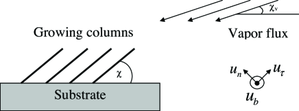
Figure 1: Schematic of the growth of a columnar thin film. The vapor flux is directed at an angle $\chi_{v}$, whereas columns grow at an angle $\chi\geq\chi_{v}$. The unit vectors ${\mathbf{u}}_{\tau}$, ${\mathbf{u}}_{n}$, and ${\mathbf{u}}_{b}$ are also shown.

2 SWP at Planar Metal–CTF Interface

Let the region $z>0$ be occupied by a CTF and the region $z<0$ by a metal of relative permittivity $\epsilon_{m}$. The relative permittivity dyadic of the CTF may be stated as [7]

$$\underline{\underline{\epsilon}}_{\,ctf}=\epsilon_{a}\,{\mathbf{u}}_{n}{\mathbf{u}}_{n}+\epsilon_{b}\,{\mathbf{u}}_{\tau}{\mathbf{u}}_{\tau}+\epsilon_{c}\,{\mathbf{u}}_{b}{\mathbf{u}}_{b}\,,$$ (1)

where $\epsilon_{a,b,c}$ are the principal relative permittivity scalars and the unit vectors

$${\mathbf{u}}_{n}=-{\mathbf{u}}_{x}\sin\chi+{\mathbf{u}}_{z}\cos\chi\,,\quad{\mathbf{u}}_{\tau}={\mathbf{u}}_{x}\cos\chi+{\mathbf{u}}_{z}\sin\chi\,,\quad{\mathbf{u}}_{b}=-{\mathbf{u}}_{y}\,.$$ (2)

All four constitutive quantities — $\epsilon_{a,b,c}$ and the column inclination angle $\chi\in\left(0,\pi/2\right]$ — depend on the evaporant species and the vapor incidence angle $\chi_{v}$. The $xz$ plane, containing the unit vectors ${\mathbf{u}}_{n}$ and ${\mathbf{u}}_{\tau}$, is the morphologically significant plane of the CTF.

In order to preserve the independence of the $p$– and the $s$–polarization states, as stated in Section 1, the wave vectors in both half–spaces must not have a component orthogonal to the morphologically significant plane. Accordingly, the $p$–polarized electromagnetic field phasors in the metal half–space are given by

$${\left.\begin{array}[]{l}{\bf E}({\bf r})=A_{m}\left({\mathbf{u}}_{x}-\frac{i\varkappa}{q_{m}}{\mathbf{u}}_{z}\right)\exp\left[ik_{\scriptscriptstyle 0}\left(\varkappa x-iq_{m}z\right)\right]\\[5.0pt] {\bf H}({\bf r})=A_{m}\,\eta_{\scriptscriptstyle 0}^{-1}\,\frac{i\epsilon_{m}}{q_{m}}\,{\mathbf{u}}_{y}\,\exp\left[ik_{\scriptscriptstyle 0}\left(\varkappa x-iq_{m}z\right)\right]\end{array}\right\}\,,\quad z\leq 0}\,,$$ (3)

where $A_{m}$ is a complex–valued scalar of finite magnitude, $q_{m}=+\sqrt{\varkappa^{2}-\epsilon_{m}}$, and $\varkappa k_{\scriptscriptstyle 0}{\mathbf{u}}_{x}$ may be regarded as the wave vector of the surface wave. We must have ${\rm Re}\left[q_{m}\right]>0$ for SWP. The $p$–polarized electromagnetic field phasors in the CTF half–space are given by [7]

$${\left.\begin{array}[]{l}{\bf E}({\bf r})=A_{c}\left[{\mathbf{u}}_{x}+\frac{i\varkappa q_{c}-(\epsilon_{a}-\epsilon_{b})\sin\chi\cos\chi}{\varkappa^{2}-(\epsilon_{a}\cos^{2}\chi+\epsilon_{b}\sin^{2}\chi)}\,{\mathbf{u}}_{z}\right]\exp\left[ik_{\scriptscriptstyle 0}\left(\varkappa x+iq_{c}z\right)\right]\\[5.0pt] {\bf H}({\bf r})=A_{c}\,\eta_{\scriptscriptstyle 0}^{-1}\left[\frac{-iq_{c}(\epsilon_{a}\cos^{2}\chi+\epsilon_{b}\sin^{2}\chi)+\varkappa(\epsilon_{a}-\epsilon_{b})\sin\chi\cos\chi}{\varkappa^{2}-(\epsilon_{a}\cos^{2}\chi+\epsilon_{b}\sin^{2}\chi)}\right]{\mathbf{u}}_{y}\,\exp\left[ik_{\scriptscriptstyle 0}\left(\varkappa x+iq_{c}z\right)\right]\end{array}\right\}\,,\quad z\geq 0}\,,$$ (4)

where $A_{c}$ is a complex–valued scalar of finite magnitude, and $q_{c}$ must be obtained by solving the quadratic equation

$$\varkappa^{2}(\epsilon_{a}\sin^{2}\chi+\epsilon_{b}\cos^{2}\chi)-2i\varkappa q_{c}(\epsilon_{a}-\epsilon_{b})\sin\chi\cos\chi-q_{c}^{2}(\epsilon_{a}\cos^{2}\chi+\epsilon_{b}\sin^{2}\chi)-\epsilon_{a}\epsilon_{b}=0\,.$$ (5)

We must choose ${\rm Re}\left[q_{c}\right]>0$ for localization of energy to the metal–CTF interface. Let us note parenthetically that $\epsilon_{c}$ does not enter our analysis.

The boundary conditions at the interface $z=0$ lead to the two equations

$${\left.\begin{array}[]{l}A_{c}=A_{m}\\[5.0pt] A_{c}\frac{-iq_{c}(\epsilon_{a}\cos^{2}\chi+\epsilon_{b}\sin^{2}\chi)+\varkappa(\epsilon_{a}-\epsilon_{b})\sin\chi\cos\chi}{\varkappa^{2}-(\epsilon_{a}\cos^{2}\chi+\epsilon_{b}\sin^{2}\chi)}=A_{m}\frac{i\epsilon_{m}}{q_{m}}\end{array}\right\}}\,,$$ (6)

which yield the dispersion equation [11]

$${\epsilon_{m}\varkappa^{2}+iq_{m}\varkappa(\epsilon_{a}-\epsilon_{b})\sin\chi\cos\chi+(q_{m}q_{c}-\epsilon_{m})(\epsilon_{a}\cos^{2}\chi+\epsilon_{b}\sin^{2}\chi)=0}$$ (7)

for SWP.

Equation (7) was solved numerically after choosing $\epsilon_{m}=-56+21i$ (typ., aluminum at $\lambda_{\scriptscriptstyle 0}=633$ nm [2]) and choosing titanium oxide as the material of which the CTF is made. At 633-nm wavelength, empirical relationships have been determined for titanium–oxide CTFs by Hodgkinson et al. [8] as

$$\epsilon_{a} = \left[1.0443+2.7394\left(\frac{\chi_{v}}{\pi/2}\right)-1.3697\left(\frac{\chi_{v}}{\pi/2}\right)^{2}\right]^{2}\,,$$ (8)

$$\epsilon_{b} = \left[1.6765+1.5649\left(\frac{\chi_{v}}{\pi/2}\right)-0.7825\left(\frac{\chi_{v}}{\pi/2}\right)^{2}\right]^{2}\,,$$ (9)

and

$$\tan\chi = 2.8818\tan\chi_{v}\,,$$ (10)

where $\chi_{v}$ and $\chi$ are in radian. We must caution that the foregoing expressions are applicable to CTFs produced by one particular experimental apparatus, but may have to be modified for CTFs produced by other researchers on different apparatuses.

Table 1 shows the computed values of the relative wavenumber $\varkappa$ for SWP on the chosen metal–CTF interface. Clearly, as $\chi_{v}$ increases towards $90^{\circ}$, both the real and the imaginary parts of $\varkappa$ increase. This means that an increase in the vapor incidence angle

• reduces the magnitude of the phase velocity and

• increases the attenuation

of the surface wave. Thus, a high value of $\chi_{v}$ is inimical to long–range SWP.

3 Modified Kretschmann Configuration

In conformance with the Kretschmann configuration [9] for launching surface plasmon polaritons, the half–space $z\leq 0$ is occupied by a homogeneous, isotropic, dielectric material described by the relative permittivity scalar $\epsilon_{1}$. Dissipation in this material is considered to be negligible and its refractive index $n_{1}=\sqrt{\epsilon_{1}}$ is real–valued and positive. The laminar region $0\leq z\leq L_{m}$ is occupied by a metal with relative permittivity scalar $\epsilon_{m}$. A CTF of relative permittivity dyadic $\underline{\underline{\epsilon}}_{\,ctf}$ occupies the region $L_{m}\leq z\leq L_{\Sigma}=L_{m}+L_{ctf}$. Finally, the half–space $z\geq L_{\Sigma}$ is taken to be occupied by an isotropic, nondissipative dielectric material with relative permittivity $\epsilon_{2}=n_{2}^{2}>0$. This modified Kretschmann configuration is in accordance with practical considerations for launching surface waves [10].

A $p$–polarized plane wave, propagating in the half–space $z\leq 0$ at an angle $\theta_{1}\in[0,\pi)$ to the $z$ axis in the $xy$ plane, is incident on the metal–coated CTF. The electromagnetic field phasors associated with the incident plane wave are represented as [7]

$$\left.\begin{array}[]{l}{\mathbf{E}}_{inc}({\bf r})=(-{\mathbf{u}}_{x}\cos\theta_{1}+{\mathbf{u}}_{z}\sin\theta_{1})\,\exp\left[i(\kappa x+n_{1}z\cos\theta_{1})\right]\\[5.0pt] {\mathbf{H}}_{inc}({\bf r})=-n_{1}\eta_{\scriptscriptstyle 0}^{-1}\,{\mathbf{u}}_{y}\,\exp\left[i(\kappa x+n_{1}z\cos\theta_{1})\right]\end{array}\right\}\,,\qquad z\leq 0\,,$$ (11)

where

$$\kappa=k_{\scriptscriptstyle 0}n_{1}\sin\theta_{1}\,.$$ (12)

The reflected electromagnetic field phasors are expressed as

$$\left.\begin{array}[]{l}{\mathbf{E}}_{ref}({\bf r})=r_{p}({\mathbf{u}}_{x}\cos\theta_{1}+{\mathbf{u}}_{z}\sin\theta_{1})\,\exp\left[i(\kappa x-n_{1}z\cos\theta_{1})\right]\\[5.0pt] {\mathbf{H}}_{ref}({\bf r})=-r_{p}\,n_{1}\eta_{\scriptscriptstyle 0}^{-1}\,{\mathbf{u}}_{y}\,\exp\left[i(\kappa x-n_{1}z\cos\theta_{1})\right]\end{array}\right\}\,,\qquad z\leq 0\,,$$ (13)

and the transmitted electromagnetic field phasors as

$$\left.\begin{array}[]{l}{\mathbf{E}}_{tr}({\bf r})=t_{p}(-{\mathbf{u}}_{x}\cos\theta_{2}+{\mathbf{u}}_{z}\sin\theta_{2})\,\exp\left\{i\left[\kappa x+n_{2}\left(z-L_{\Sigma}\right)\cos\theta_{2}\right]\right\}\\[5.0pt] {\mathbf{H}}_{tr}({\bf r})=-t_{p}\,n_{2}\eta_{\scriptscriptstyle 0}^{-1}\,{\mathbf{u}}_{y}\,\exp\left\{i\left[\kappa x+n_{2}\left(z-L_{\Sigma}\right)\cos\theta_{2}\right]\right\}\end{array}\right\}\,,\qquad z\geq L_{\Sigma}\,,$$ (14)

where $n_{2}\sin\theta_{2}=n_{1}\sin\theta_{1}=\varkappa$.

The reflection coefficient $r_{p}$ and the transmission coefficient $t_{p}$ have to be determined by the solution of a boundary–value problem [7]. It suffices to state here that the matrix equation

$$\left[\begin{array}[]{l}t_{p}\\ 0\end{array}\right]=[\underline{\underline{K}}^{(2)}]^{-1}\cdot\exp\left({i[\underline{\underline{P}}_{\,ctf}]L_{ctf}}\right)\cdot\exp\left({i[\underline{\underline{P}}_{\,m}]L_{m}}\right)\cdot[\underline{\underline{K}}^{(1)}]\cdot\left[\begin{array}[]{l}1\\ r_{p}\end{array}\right]\,$$ (15)

emerges, wherein the following 2$\times$2 matrixes are employed:

$$[\underline{\underline{K}}^{(\ell)}]=\left[\begin{array}[]{cc}-\cos\theta_{\ell}&\qquad\cos\theta_{\ell}\\[5.0pt] -n_{\ell}\,\eta_{\scriptscriptstyle 0}^{-1}&\qquad-n_{\ell}\,\eta_{\scriptscriptstyle 0}^{-1}\end{array}\right]\,,\quad\ell\in\left\{1,2\right\}\,,$$ (16)

$$[\underline{\underline{P}}_{\,m}]=\left[\begin{array}[]{cc}0&\qquad\omega\mu_{\scriptscriptstyle 0}-\frac{\kappa^{2}}{\omega\epsilon_{\scriptscriptstyle 0}\epsilon_{m}}\\[5.0pt] \omega\epsilon_{\scriptscriptstyle 0}\epsilon_{m}&\qquad 0\end{array}\right]\,,$$ (17)

$$[\underline{\underline{P}}_{\,ctf}]=\left[\begin{array}[]{cc}\frac{\kappa(\epsilon_{a}-\epsilon_{b})\sin\chi\cos\chi}{\epsilon_{a}\cos^{2}\chi+\epsilon_{b}\sin^{2}\chi}&\qquad\omega\mu_{\scriptscriptstyle 0}-\frac{\kappa^{2}}{\omega\epsilon_{\scriptscriptstyle 0}(\epsilon_{a}\cos^{2}\chi+\epsilon_{b}\sin^{2}\chi)}\\[5.0pt] \omega\epsilon_{\scriptscriptstyle 0}\frac{\epsilon_{a}\epsilon_{b}}{\epsilon_{a}\cos^{2}\chi+\epsilon_{b}\sin^{2}\chi}&\qquad\frac{\kappa(\epsilon_{a}-\epsilon_{b})\sin\chi\cos\chi}{\epsilon_{a}\cos^{2}\chi+\epsilon_{b}\sin^{2}\chi}\end{array}\right]\,.$$ (18)

The solution of (15) yields the reflection and transmission coefficients. The principle of conservation of energy mandates the constraint

$$|r_{p}|^{2}+\left(\frac{n_{2}}{n_{1}}\right)\,\left(\frac{{\rm Re}[\cos\theta_{2}]}{\cos\theta_{1}}\right)|t_{p}|^{2}\leq 1\,,$$ (19)

the inequality turning to an equality only in the absence of dissipation in the region $0<z<L_{\Sigma}$.

In order to study the excitation of a surface wave at the metal–CTF interface, the absorbance

$$A_{p}=1-\left\{|r_{p}|^{2}+\left(\frac{n_{2}}{n_{1}}\right)\,\left(\frac{{\rm Re}[\cos\theta_{2}]}{\cos\theta_{1}}\right)|t_{p}|^{2}\right\}$$ (20)

has to be plotted against the angle $\theta_{1}$. This was done for $L_{m}=10$ nm and $L_{ctf}=1000$ nm. As in Section 2, $\epsilon_{m}=-56+21i$ was chosen, along with $\epsilon_{a,b}$ and $\chi$ as specified by (8)–(10). Whereas $\epsilon_{1}=9$ was chosen to ensure that existence of a critical angle for total reflection in the absence of the 10-nm–thick metal film, $\epsilon_{2}=5$ was set for a lesser degree of constitutive contrast with the CTF.

Figure 2 shows plots of $A_{p}$ vs. $\theta_{1}$ for the same five values of $\chi_{v}$ as in Table 1. For comparison, plots of $|r_{p}|^{2}$ vs. $\theta_{1}$ in the absence of the metal film are also shown in this figure, in order to establish the critical (minimum) values of $\theta_{1}$ for total reflection. For $\theta_{1}$ greater than the critical angle for a specific $\chi_{v}$, we see very high $A_{p}$–peaks in Figure 2.

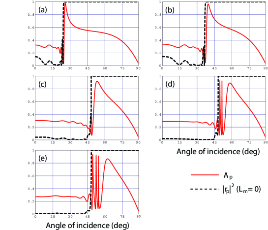
Figure 2: Solid lines represent the absorbance $A_{p}$ against the incidence incidence angle $\theta_{1}$, when $\epsilon_{1}=9$, $\epsilon_{2}=5$, $\epsilon_{m}=-56+21i$, $L_{m}=10$ nm, $L_{ctf}=1000$ nm, and $\epsilon_{a,b}$ and $\chi$ are specified by (8)–(10). Dashed lines represent $|r_{p}|^{2}$ against $\theta_{1}$ when $L_{m}=0$. (a) $\chi_{v}=5^{\circ}$, (b) $\chi_{v}=20^{\circ}$, (c) $\chi_{v}=45^{\circ}$, (d) $\chi_{v}=60^{\circ}$, (e) $\chi_{v}=90^{\circ}$.

Values of $\theta_{1}$ for the rightmost peaks of $A_{p}$ against $\chi_{v}$ in Figure 2 are provided in Table 2, along with the corresponding values of $\varkappa=n_{1}\sin\theta_{1}$. The values of $\varkappa$ in Table 2 are quite close to the real parts of those in Table 1, thereby indicating that the rightmost $A_{p}$–peaks in Figure 1 can be attributed to the excitation of surface waves at the planar metal–CTF interface [2]. Not surprisingly, the value of $\theta_{1}$ needed to excite a surface wave in the modified Kretschmann configuration increases as the vapor incidence angle $\chi_{v}$ gets closer to $90^{\circ}$.

4 Concluding Remarks

Right from the time of Faraday [12], morphology is widely known to play a key role in the optical responses of thin films [13-15]. More recently, Hodgkinson and Wu made a comprehensive proposal to regard columnar thin films as equivalent to biaxial crystals [6], which functional analogy can be extended to sculptured thin films [7]. Therefore, it is appropriate that the excitation of surface waves at the planar interfaces of isotropic dielectric materials [10] and metals with CTFs be influenced by morphology. In this communication, we have shown that the selection of a higher vapor deposition angle when growing the CTF, with consequent influence on the morphology of the CTF, will lead to a surface wave at a planar metal–CTF interface with phase velocity of lower magnitude and shorter propagation range; concomitantly, a higher incidence angle will be required to excite that surface wave in a modified Kretschmann configuration.

Acknowledgment. This communication is dedicated to Prof. Prasad Khastgir, a great teacher of physics.

References

1. Zenneck J, Ann. Phys. Lpz. 23 (1907) 846.

2. Mansuripur M, Li L, OSA Opt. Photon. News 8 (1997) 50 (May issue).

3. Pitarke J M, Silkin V M, Chulkov E V, Echenique P M, Rep. Prog. Phys. 70 (2007) 1.

4. Singh J, Thyagarajan K, Opt. Commun. 85 (1991) 397.

5. Mihalache D, Baboiu D-M, Ciumac M, Torner L, Torres J P, Opt. Quant. Electron. 26 (1994) 857.

6. Hodgkinson I J, Wu Q h, Birefringent thin films and polarizing elements. (World Scientific, Singapore), 1997.

7. Lakhtakia A, Messier R, Sculptured thin films: Nanoengineered morphology and optics. (SPIE Press, Bellingham, WA, USA), 2005, Chap. 7.

8. Hodgkinson I J, Wu Q h, Hazel J, Appl. Opt. 37 (1998) 2653.

9. Kretschmann E, Raether H, Z. Naturforsch. A 23 (1968) 2135.

10. Simon H J, Mitchell D E, Watson J G, Am. J. Phys. 43 (1975) 630.

11. Polo Jr J A, Nelatury S R, Lakhtakia A, J. Nanophoton. 1 (2007) 013501.

12. Faraday M, Phil. Trans. R. Soc. Lond. 147 (1857) 145.

13. Heavens O S, Optical properties of thin solid films. Dover Publications, Mineola, NY, USA), 1965.

14. Ward L, The optical constants of bulk materials and films. (Institute of Physics Publishing, Bristol, United Kingdom), 1994.

15. Rancourt J D, Optical thin films: User handbook. (SPIE Press, Bellingham, WA, USA), 1996.