Searching for Gravitational-Wave Bursts with LIGO

We present recent results from searches by the LIGO Science Collaboration for bursts of gravitational-wave radiation, as well as the status of other ongoing searches. These include directed searches for bursts associated with observed sources (gamma-ray bursts, soft gamma repeaters) and untriggered searches for bursts from unknown sources. We also present the status of some newer investigations, such as coherent network methods. We show methods for interpreting our search results in terms of astrophysical source distributions that improve their accessibility to the wider community.

1 Introduction

The Laser Interferometer Gravitational Wave Observatory (LIGO) is in the middle of a lengthy science run (S5) in the search for gravitational-wave (GW) signals. One class of signals are short-duration ($<1$ sec) “bursts” of gravitational-wave energy. The LIGO Science Collaboration (LSC), an international organization of researchers working with the LIGO $\!{}^{{\bf?}}$ and GEO 600 $\!{}^{{\bf?}}$ detectors, is continuing searches for these GW bursts started in previous science runs. Section 2 reviews recent progress and results from LIGO-only searches. The remainder of the paper discusses some examples of new analysis directions being pursued by members of the LSC. Section 3 covers new work on network-based burst searches, looking towards the addition of data from GEO 600, Virgo $\!{}^{{\bf?}}$, and eventually other observatories. The last section covers methods for presenting GW burst search results in terms of rate limits for models of astrophysical source distributions.

2 Recent LIGO GW Burst Searches

Unlike the well-modeled waveforms for GW signals from pulsars and the inspiral phase of binary compact object mergers, GW bursts are poorly modeled at present. Searches for GW burst signals thus must remain sensitive to a large range of signal waveforms. We divide the searches into two classes. One class are untriggered searches that examine all sky locations at all observation times. The other class are directed searches for GW burst signals associated with astronomically-identified source candidates such as Gamma-Ray Bursts (GRBs) of known sky location and observation time.

2.1 All-Sky Untriggered Burst Search

The initial untriggered burst search for LIGO run S5 uses the same approach as was used for runs S2, S3, and S4 $\!{}^{{\bf?}}$. The search starts with a wavelet decomposition of the gravitational-wave channel data from each detector separately into time-frequency maps. Samples (“pixels”) from these maps that have excess signal power relative to the background are identified. Such pixel clusters that are coincident in time and frequency between all three LIGO interferometers are selected as candidate triggers for further analysis. The candidate triggers must then pass a set of signal consistency tests. Based around pair-wise cross- correlation tests, these confirm that consistent waveforms and amplitudes are seen in all interferometers. These same methods are used to measure background rates by processing data with many artificial time shifts between the two LIGO sites in Hanford (Washington) and Livingston (Louisiana).

The LIGO-only burst GW analysis can have significant backgrounds from non-Gaussian transients. A particular problem are environmental transients at the Hanford site. These can induce simultaneous large- amplitude signals in the co-located interferometers (labeled H1 and H2) at that location. Detailed studies of Data Quality (DQ) are required to identify and define time intervals when such problems are present. This work is assisted by the large number of auxiliary channels of interferometer and environmental sensor data that are recorded during science operation. Longer-duration time periods that have known artifacts or unreliable interferometer data are flagged as DQ Period Vetoes. Short-duration transient events in the auxiliary channels that are found to be associated with events in the GW channels are flagged as Auxiliary-Channel Event Vetoes. Both veto classes are used to reject GW Burst triggers that coincide with them. These vetoes help remove any large-amplitude outliers in the final GW Burst trigger samples $\!{}^{{\bf?}}$.

A detailed analysis of untriggered burst search results from the early part of S5 operation is being completed for publication. We note that our searches in the previous LIGO runs (S1 $\!{}^{{\bf?}}$, S2 $\!{}^{{\bf?}}$, S3 $\!{}^{{\bf?}}$ and S4 $\!{}^{{\bf?}}$) did not see any GW burst signals. The S5 run has both greater sensitivity than previous runs and at least 10 times the observation time. As in S4, this initial S5 all-sky GW burst search is tuned by bursts $\ll 1$ sec in duration over a frequency range of 64-1600 Hz. As there are few well-modeled waveforms for bursts from theoretical studies, we use ‘ad-hoc’ waveforms such as Gaussian-envelope sine- waves (sine-Gaussians) and Gaussians that mimic the expected transient response to such bursts. We measure our sensitivity to such ad-hoc waveforms in terms of their root-sum-squared amplitude ($h_{rss}$) which is in units of $\mbox{strain}/\sqrt{\mbox{Hz}}$ defined as

$$h_{rss}=\sqrt{\int(|h_{+}(t)|^{2}+|h_{\times}(t)|^{2})dt}\,.$$ (1)

The “efficiency” of an analysis is the probability that it will successfully identify a signal with certain specified parameters. For an all-sky search, we use a Monte Carlo approach to evaluate the efficiency for each of these waveforms as a function of amplitude, averaging over sky position and polarization angle. This information is used to derive exclusion diagrams that place bounds on the event rate as a function of $h_{rss}$. This is shown in Fig. 1, taken from our recent S4 paper  $\!{}^{{\bf?}}$.

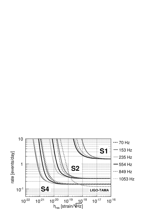
Figure 1: Exclusion diagram (rate limit at 90% confidence level, as a function of signal amplitude) for sine-Gaussian simulated waveforms for S1, S2 and S4 LIGO GW burst analyses (No rate limit quoted in S3 analysis).

In our early S5 analysis, we are achieving detection sensitivities of $h_{rss}<10^{-21}\,\mbox{strain}/\sqrt{\mbox{Hz}}$ for some of the ad-hoc waveforms considered. These instrumental sensitivities can also be converted to corresponding energy emission sensitivity $\!{}^{{\bf?}}$. Assuming (for simplicity) isotropic emission at a distance $R$ by GW bursts with sine-Gaussian waveforms, we have

$$E_{GW}=(2.1M_{\odot}c^{2})\left(\frac{R}{100\,\mbox{Mpc}}\right)^{2}\left(\frac{f}{100\,\mbox{Hz}}\right)^{2}\left(\frac{h_{rss}}{10^{-21}\,\mbox{Hz}^{-1/2}}\right)^{2}$$ (2)

During the early part of S5, we are sensitive to $E_{GW}\sim 0.1M_{\odot}c^{2}$ at a distance of 20 Mpc for $f=153$ Hz sine-Gaussians.

2.2 GRB-triggered Burst Search

We have completed a search for short-duration GW bursts that are coincident with Gamma-Ray Bursts (GRBs) from the data in several previous LIGO science runs (S2, S3 and S4). This analysis used pair-wise cross-correlation of signals from two LIGO interferometers, as used in our search for gravitational waves associated with GRB030209 $\!{}^{{\bf?}}$. This approach increased the observation time over that available when all three LIGO interferometers were in science mode. The search targeted bursts with durations 1 to 100 ms over a bandwidth of 40–2000 Hz. The sensitivity of this GRB search is similar to that of the untriggered search. As well as setting limits on GW bursts from individual GRBs, it was demonstrated that multiple GRBs can be combined to obtain an upper limit on GRB population parameters. During S5, there have been about 10 GRBs per month. Thus, the GRB sample that will be used in the S5 analysis will be much larger.

2.3 SGR 1806–20 Search

We have also completed a search for GW signals associated with the Soft Gamma-Ray Repeater (SGR) 1806–20. This SGR had a record flare on December 27, 2004 $\!{}^{{\bf?}}$. During this flare, quasi-periodic oscillations (QPOs) were seen in X-ray data from the RHESSI and RXTE satellites. These QPOs lasted for hundreds of seconds. During this flare, only one LIGO detector (H1) was observing. A band-limited excess-power search was conducted for quasi-periodic GW signals coincident with the flare $\!{}^{{\bf?}}$. No evidence was found for GW signals associated with the QPOs. Our sensitivity to the 92.5 Hz QPO was $E_{GW}\sim 10^{-7}\mbox{ to }10^{-8}M_{\odot}$, based on the 5–10 kpc distance of SGR 1806–20. This is comparable to the total electro-magnetic energy emitted in the flare.

3 Coherent GW Burst Searches

The existing LIGO all-sky untriggered and GRB triggered burst search pipelines have been operating continuously on the acquired science- mode data since the start of the S5 run. These provide for the chance of prompt detection of GW bursts, enabling timely follow-up and investigation. The results are also used to provide identification of false signals from transients, speeding up the data quality and auxiliary-channel veto studies.

In searching for GW bursts, the community is adopting an approach that might be termed “The Network is the Observatory”. The benefit of having observatories at multiple, widely-separated locations cannot be stressed enough. While LIGO-only burst searches have been fruitful, they require intense investigations for environmental and interferometer transients to remove backgrounds. Our previous LSC analyses have not made full use of the constraints that a network of sites can jointly make simultaneously on $h_{+}$ and $h_{\times}$ waveforms. Specifically, the GW burst searches must prepare for the inclusion of data from the GEO 600 and Virgo observatories, and others in the future.

We fully expect to move from the era of upper limits to that of detection. In moving to detection, GW burst searches need to extract the waveform of the signals that are detected. Such waveforms can be compared to those from theoretical predictions for potential identification of the source type. We may also provide interpretations of our GW burst results in terms of rates from astrophysical source distributions.

3.1 Coherent Network Burst Searches

A coherent method for GW burst searches was first proposed by Gürsel and Tinto $\!{}^{{\bf?}}$, where they combined the detector responses into a functional. This functional minimizes in the direction of the source and allows extraction of both the source coordinates and the two polarization components of the burst signal waveform. Flanagan and Hughes $\!{}^{{\bf?}}$ expanded this to the maximization of a likelihood functional over the space of all waveforms. Using simulated data, Arnaud et al  $\!{}^{{\bf?}}$ found that coherent methods were more efficient than coincidence methods for burst signals, in an exploration of their statistical performance. Within the LSC, there has been substantial work to develop searches that evaluate the network’s composite response to GW burst signal. Such “coherent network” techniques can accommodate arbitrary networks of detectors and will be among the methods used by the LSC for the analysis of the S5 data.

To describe coherent network burst searches, we will follow the presentation in Klimenko et al $\!{}^{{\bf?}}$. In the coordinate frame associated with the wave (termed the wave frame), a gravitational wave propagates in the direction of the $z$ axis. For a specific source, the $z$-axis is defined by the source’s location on the sky in terms of angles $\theta$ and $\phi$. The wave can be described with the $h_{+}$ and $h_{\times}$ waveforms representing the two independent polarization components of the wave. In describing the network analysis, we will use complex waveforms defined as

$$u(t) = h_{+}(t)+ih_{\times}(t)$$ (3)

$$\tilde{u}(t) = h_{+}(t)-ih_{\times}(t)$$ (4)

We use a tilde($\tilde{\,}$) to indicate the complex conjugate. These complex waveforms are eigenstates of the rotations about the $z$ axis in the wave frame.

The response $\xi(u)$ of an individual detector can be expressed conveniently in terms of these complex waveforms:

$$\xi(u)=\tilde{A}u+A\tilde{u}$$ (5)

where $A$ and $\tilde{A}$ are complex expressions of the standard antenna patterns. We note that this detector response is invariant under rotations $R_{z}$ in the wave frame. This can be extended to a network of detectors, where the response from each detector is weighted by its noise variance $\sigma^{2}$. We combine the per-detector antenna patterns into the network antenna patterns

$$g_{r}=\sum_{k=1}^{K}\frac{A_{k}\tilde{A}_{k}}{\sigma_{k}^{2}},\;g_{c}=\sum_{k=1}^{K}\frac{A_{k}^{2}}{\sigma_{k}^{2}}$$ (6)

where $g_{r}$ is real and $g_{c}$ is complex. The analogous network response $R(u)$ is expressed in terms of these patterns:

$$R(u)=g_{r}u+g_{c}\tilde{u}$$ (7)

There is also the network output time series $X$ that combines the output time-series $x_{k}$ from each detector

$$X=\sum_{k=1}^{K}\frac{x_{k}A_{k}}{\sigma_{k}^{2}}$$ (8)

The equations for the GW waveforms from the network are obtained by variation of the likelihood functional. This results in two linear equations for $u$ and $\tilde{u}$

$$X = g_{r}u+g_{c}\tilde{u}$$ (9)

$$\tilde{X} = g_{r}\tilde{u}+\tilde{g}_{c}u$$ (10)

These can be written in matrix form as

$$\left[\begin{array}[]{ c }Re(X)\\ Im(X)\end{array}\right]=M_{R}\left[\begin{array}[]{ c }h_{+}\\ h_{\times}\end{array}\right]$$ (11)

where $M_{R}$ is the network response matrix.

The invariance of the response to an arbitrary rotation $R_{z}(\psi)$ through an angle $\psi$ allows us to select the rotation in which both network antenna patterns $g_{r}$ and $g_{c}$ are real and positively defined. This simplifies the network response to

$$R=(g_{r}+|g_{c}|)h_{1}+i(g_{r}-|g_{c}|)h_{2}$$ (12)

where $h_{1}$ and $h_{2}$ are the real and imaginary components of the signal. That leads to a diagonal form for the network response matrix:

$$M_{R}=g\left(\begin{array}[]{ c c }1&0\\ 0&\epsilon\end{array}\right)$$ (13)

The coefficient $g$ characterizes the network sensitivity to the $h_{1}$ wave. The sensitivity to the $h_{2}$ wave is $\epsilon g$, where $\epsilon$ is the network alignment factor. For most sources, the $h_{1}$ and $h_{2}$ components should have similar amplitudes.

However, there is a problem in the use of coherent network approaches that is most acute for a network of two detector locations, such as the LIGO-only configuration with detectors at Hanford and Livingston. It has been shown $\!{}^{{\bf?}}$ that if the detectors are even slightly misaligned, the normal likelihood statistic becomes insensitive to the cross-correlation between the detectors. This results in the network alignment factor $\epsilon$ being $\ll 1$ for most sky location angles $\theta$ and $\phi$, and hence the network being insensitive to the $h_{2}$ wave component. This problem lessens somewhat as more detectors, such as GEO 600 and Virgo, are added, but does not disappear.

3.2 Application to Untriggered Burst Search

One method that has been developed to deal with the relative insensitivity to the $h_{2}$ component is the “constraint likelihood” $\!{}^{{\bf?}}$. This applies a “soft constraint” on the solutions that penalizes the unphysical solutions with $h_{1}=0$ that would be consistent with those produced by noise. This sacrifices a small fraction of the GW signals but enhances efficiency for the rest of the sources.

The existing wavelet-based search has been converted into an all-sky coherent network search using this “constraint likelihood” technique. It can handle arbitrary networks of detectors and has been tested on existing data from the LIGO and GEO 600 detectors. This all-sky coherent network search also divides the detected energy from all detectors into coherent and incoherent components. A cut on the network correlation (coherent / total) further removes backgrounds from single-detector transients. When compared to our existing all-sky search method for S5, this coherent network search achieves equal or better sensitivity with a very low background rate. Other coherent search methods have also been explored and/or implemented $\!{}^{{\bf?},{\bf?},{\bf?}}$.

3.3 Application to Triggered Burst Search

Additional methods for handling the $h_{1}$ and $h_{2}$ polarization components in the likelihood have been studied $\!{}^{{\bf?},{\bf?}}$. It was noted that problems arise when the inversion of the detector response to obtain the waveforms is ill-posed due to “rank deficiency”. This can be solved using many types of regularization.

The method of Tikhonov regularization $\!{}^{{\bf?}}$ is used in a new triggered coherent network analysis $\!{}^{{\bf?}}$ developed by the LSC for S5 and subsequent data sets. Because there is prior knowledge of the sky locations, and fewer sources than in the untriggered analysis, more computationally intensive methods can be used. In fact, some additional network analysis methods are under development for the triggered burst search.

4 Astrophysical Interpretation

The existing GW burst search results from LIGO (See Fig. 1) have been reported in terms of detector-centric “Rate vs. Strength” exclusion curves. These methods say nothing about the sources of GW bursts or about the absolute rate of source events. The “Rate”, typically in events/day, is only meaningful if all events are assumed to have the same “Strength”, i.e. GW strain amplitude at the Earth, expressed in terms of $h_{rss}$. This strength parameter reveals little about source quantities such as the absolute luminosity in terms of emitted gravitational-wave energy.

Alternatively, we could report results in terms of rates from a source population as a function of the intrinsic energy radiated. We note that interpretation, astrophysical or otherwise, is always in terms of a model. The components of such a model would be the source population distribution and the source strain energy spectrum appropriate for GW burst searches. We also need to add in the observation schedule. This schedule is the sidereal time associated with the data that is analyzed, that provides the detector pointing relative to the source population distribution.

We wish to report results in terms of their Astrophysical Rate vs. Strength. The Astrophysical Rate is the event rate in the source population. The Astrophysical Strength is an astrophysically meaningful amplitude parameter such as the radiated energy. We express the bound on the astrophysical rate vs strength

$$R(E)=\frac{k}{T_{obs}\epsilon(E)}$$ (14)

where the constant $k$ is set by the number of observed events (2.3 for no observed events), $T_{obs}$ is the total observation time and $\epsilon(E)$ is the efficiency in the population. The efficiency in the population is the ratio of the expected number of observed sources over the total number of sources. The expected number of observed sources is the integral of the source rate distribution over detection efficiency and observation schedule. The total number of sources is the integral of the source rate distribution over the observation schedule alone. The source rate distribution will be a function of location, orientation and luminosity.

4.1 Example of Astrophysical Interpretation

It is best to illustrate what an astrophysical interpretation means with an example. We start by choosing a source population. We will assume the source population traces out the old stellar population. We will thus use a Milky Way galactic model with a thin disk, thick disk, bulge, bar and halo that are characteristic of the observed white dwarf population. For a source model, we will assume an implusive event that involves stellar-mass compact objects. These events could be supernovae, accretion-induced collapses (AIC), etc. We will assume axisymmetric GW bursts and “standard candle” amplitudes, i.e. each source has the same absolute luminosity in GW energy. For the network of detectors, we assume interferometers at the LIGO Hanford, LIGO Livingston and Virgo Cascina sites. Each site has an interferometer (labeled H1, L1 and V1) with a detection sensitivity characterized as a step-function at $h_{rss}\sim 10^{-20}\,\mbox{Hz}^{-1/2}$. The LIGO Hanford site has an additional interferometer (H2) that has $h_{rss}\sim 2\times 10^{-20}\,\mbox{Hz}^{-1/2}$ due to being half as long as H1. For this example, we will assume a 100% observation schedule, implying uniform coverage in sidereal time.

First we calculate the efficiency to the population $\epsilon(E)$ as a function of the energy radiated ($E$). This is shown in Fig. 2 which has the efficiency broken down by contributions from each galactic model component to the total as a function of radiated energy in solar masses.

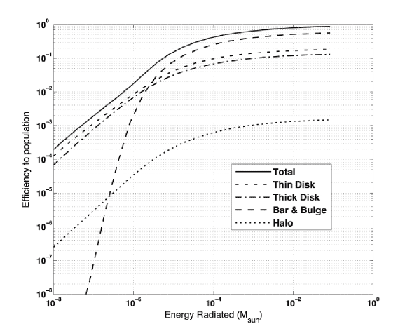
Figure 2: Detection efficiency for the example galactic source population model described in the text. Note how disk components dominate at low levels of intrinsic radiated energy, while bar and bulge components dominate for larger levels of radiated energy.

Note in our example that for radiated energy above $10^{-5}$ solar masses, contributions from the bar and bulge components dominate, while below $10^{-6}$ solar masses, the thin and thick disk components dominate.

The efficiency to the population is used to derive the bound on population rate vs. strength. This is shown in Fig. 3 for the example.

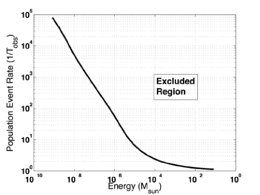
Figure 3: Bound on Population Event Rate as a function of Radiated Energy.

As different components dominate, the shape of the exclusion curve changes.

5 Conclusions

The LIGO-based burst searches are well established and already processing the data from the current S5 science run. New network-based techniques have been developed that provide enhanced detection sensitivity and background rejection. These methods show our preparation for joint observation with the Virgo observatory. The introduction of results interpretation in terms of astrophysical source distributions improves their accessibility to the astronomy and astrophysics communities.

References

References

- [1] Sigg D (for the LSC), Class. Quant. Grav. 23, S51-S56 (2006)
- [2] Lück H et al, Class. Quant. Grav. 23, S71-S78 (2006)
- [3] Acernese F et al, Class. Quant. Grav. 23, S63-S69 (2006)
- [4] Abbott B et al (LSC), Search for gravitational-wave bursts in LIGO data from the fourth science run, submitted to Classical and Quantum Gravity, preprint arXiv:0704.0943 [gr-qc]
- [5] Abbott B et al (LSC), Phys. Rev. D 69, 102001 (2004)
- [6] Abbott B et al (LSC), Phys. Rev. D 72, 062001 (2005)
- [7] Abbott B et al (LSC), Class. Quant. Grav. 23, S29-S39 (2006)
- [8] Riles K LIGO technical document LIGO-T040055-00-Z (2004)
- [9] Abbott B et al (LSC), Phys. Rev. D 72, 042002 (2005)
- [10] Hurley K et al, Nature 434, 1098-1103 (2005)
- [11] Abbott B et al (LSC), submitted to Phys. Rev. D, preprint astro-ph/0703419.
- [12] Y. Gürsel and M. Tinto, Phys. Rev. D 40, 3884 (1989)
- [13] É. Flanagan and S. A. Hughes, Phys. Rev. D 57, 4535 (1998)
- [14] N. Arnaud et al, Phys. Rev. D 68, 102001 (2003)
- [15] S. Klimenko, S. Mohanty, M. Rakhmanov, G. Mitselmakher, Phys. Rev. D 72, 122002 (2005)
- [16] W. G. Anderson, P. R. Brady, J. D. E. Creighton, and É É Flanagan, Phys. Rev. D 63, 042003 (2001)
- [17] L. Wen and B. Schutz, Class. Quant. Grav. 22, S1321-S1335 (2005)
- [18] S. Chatterji, A. Lazzarini, L. Stein, P. J. Sutton, and A. Searle, Phys. Rev. D 74, 082005 (2006)
- [19] S. Mohanty, M. Rakhmanov, S. Klimenko, G. Mitselmakher, Class. Quant. Grav. 23, 4799-4810 (2006)
- [20] M. Rakhmanov, Class. Quant. Grav. 23, S673-S686 (2006)
- [21] K. Hayama, S. Mohanty, M. Rakhmanov, S. Desai, Coherent network analysis for triggered gravitational wave burst searches (to be submitted to Classical and Quantum Gravity)