A Metric on Shape Space with Explicit Geodesics

Abstract.

This paper studies a specific metric on plane curves that has the property of being isometric to classical manifold (sphere, complex projective, Stiefel, Grassmann) modulo change of parametrization, each of these classical manifolds being associated to specific qualifications of the space of curves (closed-open, modulo rotation etc…) Using these isometries, we are able to explicitely describe the geodesics, first in the parametric case, then by modding out the paremetrization and considering horizontal vectors. We also compute the sectional curvature for these spaces, and show, in particular, that the space of closed curves modulo rotation and change of parameter has positive curvature. Experimental results that explicitly compute minimizing geodesics between two closed curves are finally provided

Introduction

The definition and study of spaces of plane shapes has recently met a large amount of interest [2, 5, 7, 10, 18, 15], and has important applications, in object recognition, for the analysis of shape databases or in medical imaging. The theoretical background involves the construction of infinite dimensional manifolds of shapes [7, 15]. The Riemannian framework, in particular, is appealing, because it provides shape spaces with a rich structure which is also useful for applications. A general discussion of several classes of metrics that can be introduced for this purpose can be found in [11].

The present paper focuses on a particular Riemannian metric that has very specific properties. This metric, which will be described in the next section, can be seen as a limit case of one of the classes studied in [11], and would receive the label $H_{1,\infty}$ in the nomenclature introduced therein. One of its surprising properties is that it can be characterized as a image of a Grassmann manifold by a suitably chosen Riemannian submersion. A consequence of this is the possibility to derive explicit geodesics in this shape space.

A precursor of the $H_{1,\infty}$ metric has been introduced in [18, 19] and studied in the context of open plane curves. It has also recently been used in [12]. Because the metric is placed on curves modulo changes of parametrization, the computation of geodesics naturally provides an elastic matching algorithm.

The paper is organized as follows. We first provide the definitions and notation that we will use for spaces of curves, the $H_{1,\infty}$ metric and the classical manifolds that will be shown to be isometric to it. We then study some local properties of the obtained manifold, discussing in particular its geodesics and sectional curvature. We finally provide experimental results for the numerical computation of geodesics and the solution of the related elastic matching problem.

1. Spaces of Curves

Throughout this paper, we will assume our plane curves are curves in the complex plane $\mathbb{C}$. Then real inner products and $2\times 2$ determinants of real 2-vectors are given by $\langle x,y\rangle=\operatorname{Re}(\bar{x}y)$ and $\det(x,y)=\operatorname{Im}(\bar{x}y)$.

We first recall the notations for various spaces of plane curves which we will need, some of which were introduced in the previous paper [11]. For all questions about infinite dimensional analysis and differential geometry we refer to [9]. By

$$\operatorname{Imm}_{\text{op}}=\operatorname{Imm}([0,2\pi],\mathbb{C})$$

we denote the space of $C^{\infty}$-immersions $c:[0,2\pi]\rightarrow\mathbb{C}$. Here ‘op’ stands for open curve. $B_{i,\text{op}}$ is the quotient of $\operatorname{Imm}_{\text{op}}$ by the group $\text{Diff}^{+}([0,2\pi])$ of $C^{\infty}$ increasing diffeomorphisms of $[0,2\pi]$. Next

$$\operatorname{Imm}_{{\text{ev}}}(S^{1},\mathbb{C}),\quad\operatorname{Imm}_{{\text{od}}}(S^{1},\mathbb{C})$$

are the spaces of $C^{\infty}$-immersions $c:S^{1}\rightarrow\mathbb{C}$ of even, respectively odd rotation degree. Here, $S^{1}$ is the unit circle in $\mathbb{C}$, which will be identified in this paper to $\mathbb{R}/(2\pi\mathbb{Z})$. Then $B_{i,{\text{ev}}}$ and $B_{i,{\text{od}}}$ are the quotients of $\operatorname{Imm}_{\text{ev}}$, respectively $\operatorname{Imm}_{\text{od}}$ by the group $\text{Diff}^{+}(S^{1})$ of $C^{\infty}$ orientation preserving diffeomorphisms of $S^{1}$. For example, $B_{i,{\text{od}}}$ contains the simple closed plane curves, since they have index +1 or $-1$ (depending on how they are oriented). These are the main focus of this study. To save us from enumerating special cases, we will often consider open curves as defined on $S^{1}$ but with a possible discontinuity at 0. We will also consider the quotients of these spaces by the group of translations, by the group of translations and rotations and the group of translations, rotations and scalings.

Using the notation of [11], we can introduce the basic metric studied in this paper on these three spaces of immersions, but modulo translations, as follows. Identify $T_{c}(\operatorname{Imm}/\text{transl})$ with the set of vector fields $h:S^{1}\rightarrow\mathbb{C}$ along $c$ modulo constant vector fields. Then we consider the limiting case of the scale invariant metric of Sobolev order 1 from [11], 4.8:

(1) $$G_{c}(h,h)=G^{\mathrm{imm,scal},1,\infty}_{c}(h,h)=\frac{1}{\ell(c)}\int_{S^{1}}|D_{s}h|^{2}.ds$$

where, as in [11], $ds=|c_{\theta}|\,d\theta$ is arclength measure, $D_{s}=D_{s,c}=|c_{\theta}|^{-1}\partial_{\theta}$ is the derivative with respect to arc length, and $\ell(c)$ is the length of $c$. We also recall for later use the notation $v=c_{\theta}/|c_{\theta}|$ for the unit tangent vector, and, as multiplication by $i$ is rotation by 90 degrees, $n=i.v$ for the unit normal. Note that this metric is invariant with respect to reparametrizations of the curve $c$, hence it induces a metric which we also call $G$ on the quotient spaces $B_{i,\text{op}},B_{i,{\text{ev}}}$ and $B_{i,{\text{od}}}$ also modulo translations.

The geodesic equation in all these metrics is a simple limiting case of those worked out in [11]. Suppose $c(\theta,t)$ is a geodesic. Then:

$$c_{tt}=D_{s}^{-1}\left(\langle D_{s}c_{t},v\rangle D_{s}c_{t}-\tfrac{1}{2}|D_{s}c_{t}|^{2}v\rangle\right)-\overline{\left\langle{\langle D_{s}c_{t},v\rangle}\right\rangle}.c_{t}-\frac{1}{2}\overline{\left\langle{|D_{s}c_{t}|^{2}}\right\rangle}.D_{s}^{-2}(\kappa.n)$$

Here the bar indicates the average of the quantity over the curve $c$, i.e. $\overline{\left\langle{F}\right\rangle}=\tfrac{1}{\ell}\int Fds$. Unfortunately, this case was not worked out in [11], hence we give the details of its derivation in Appendix I. The local existence and uniqueness of solutions to this equations can be proved easily, essentially because of the regularizing influence of the term $D_{s}^{-1}$. This will also follow from the explicit representation of these geodesics to be given below, but because of its more general applicability, we give a direct proof in Appendix I.

It is convenient to introduce the momentum $u=-D_{s}^{2}(c_{t})$ associated to a geodesic. Using the momentum, the geodesic equation is easily rewritten in the more compact form:

$$u_{t}=-\langle u,D_{s}c_{t}\rangle v-\left(\langle D_{s}c_{t},v\rangle-\overline{\left\langle{\langle D_{s}c_{t},v\rangle}\right\rangle}\right)u-\frac{1}{2}\left(|D_{s}c_{t}|^{2}+\overline{\left\langle{|D_{s}c_{t}|^{2}}\right\rangle}\right)\kappa(c).n.$$

By the theory of Riemannian submersions, geodesics on the quotient spaces $B_{i}$ are nothing more than horizontal geodesics in $\operatorname{Imm}$, that is geodesics which are perpendicular at one hence all points to the orbit of the group of reparametrizations. As is shown in [11], horizontality is equivalent to the condition $u=a.n$ for some scalar function $a(\theta,t)$. Substituting $u=a.n$ and taking the $n$-component of the last equation, we find that horizontal geodesics are given by:

$$a_{t}=-a\left(\langle D_{s}c_{t},v\rangle-\overline{\left\langle{\langle D_{s}c_{t},v\rangle}\right\rangle}\right)+\frac{\kappa(c)}{2}\left(|D_{s}c_{t}|^{2}+\overline{\left\langle{|D_{s}c_{t}|^{2}}\right\rangle}\right).$$

There are several conserved momenta along each geodesic $t\mapsto c(\theta,t)$ of this metric (see [11], 4.8): The ‘reparametrization’ momentum is

$$\frac{-1}{\ell(c)}\langle c_{\theta},D_{s,c}^{2}c_{t}\rangle|c_{\theta}|$$

which vanishes along all horizontal geodesics. The translation momentum vanishes because the metric does not feel translation (constant vector fields along $c$). The angular momentum is

$$\frac{-1}{\ell(c)}\int_{S^{1}}\langle i.c,D^{2}_{s,c}c_{t}\rangle\,ds=\frac{1}{\ell(c)}\int_{S^{1}}\kappa\langle v,c_{t}\rangle\,ds.$$

Since the metric invariant under scalings, we also have the scaling momentum

$$\frac{-1}{\ell(c)}\int_{S^{1}}\langle c,D_{s,c}^{2}c_{t}\rangle\,ds=\partial_{t}\log\ell(t).$$

So we may equivalently consider either the quotient space $\operatorname{Imm}/\text{translations}$ or consider the section of the translation action $\{c\in\operatorname{Imm}:c(0)=0\}$. In the same way, we may either pass modulo scalings or consider the section by fixing $\ell(c)=1$, since the scaling momentum vanishes here. Finally, in some cases, we will pass modulo rotations. We could consider the section where angular momentum vanishes: but this latter is not especially simple

2. The Basic Mapping for Parametrized Curves

2.1. The basic mapping

We introduce the three function spaces:

$$V_{\text{op}} =\text{Vector space of all }C^{\infty}\text{ mappings }f:[0,2\pi]\rightarrow\mathbb{R}$$

$$V_{{\text{ev}}} =\text{Vector space of all }C^{\infty}\text{ mappings }f:S^{1}\rightarrow\mathbb{R}\text{ such that }f(\theta+2\pi)\equiv f(\theta)$$

$$V_{{\text{od}}} =\text{Vector space of all }C^{\infty}\text{ mappings }f:S^{1}\rightarrow\mathbb{R}\text{ such that }f(\theta+2\pi)\equiv-f(\theta)$$

All three spaces have the weak inner product:

$$\|f\|^{2}=\int_{0}^{2\pi}f(x)^{2}dx.$$

Given $e,f$ from any of these spaces, the basic map is:

$$\Phi:(e,f)\longmapsto c(\theta)=(1/2)\int^{\theta}_{0}\left(e(x)+if(x)\right)^{2}dx.$$

The map $c$ so defined carries $[0,2\pi]$ or $S^{1}$ to $\mathbb{C}$. It need not be an immersion, however, because $e$ and $f$ might vanish simultaneously. Define

$$Z(e,f)=\{\theta:e(\theta)=f(\theta)=0\}.$$

Then we get three maps:

$$\{(e,f)\in V\times V:Z(e,f)=\emptyset\}\longrightarrow\operatorname{Imm}_{x},\text{ for }V=V_{\text{op}},V_{\text{ev}},V_{\text{od}}.$$

Looking separately at the three cases, define first the sphere $\operatorname{\bf S}(V^{2}_{\text{op}})$ to be the set of $(e,f)\in V_{\text{op}}^{2}$ such that $\|e\|^{2}+\|f\|^{2}=2$. $\operatorname{\bf S}^{0}(V^{2}_{\text{op}})$ is defined as the subset where $Z(e,f)=\emptyset$. Then the magic of the map $\Phi$ is shown by the following key fact [18]:

2.2 Theorem.

$\Phi$ defines a map:

$$\Phi:\operatorname{\bf S}^{0}(V^{2}_{\text{op}})\longrightarrow\left\{c\in\operatorname{Imm}_{\text{op}}:\ell(c)=1,c(0)=0\right\}\cong\operatorname{Imm}_{\text{op}}\Big{/}(\text{transl,scalings})$$

which is an isometric 2-fold covering, using the natural metric on $\operatorname{\bf S}$ and the metric $G^{\mathrm{imm,scal},1,\infty}$ on $\operatorname{Imm}_{\text{op}}$.

Proof. The mapping $\Phi$ is surjective: Given $c\in\operatorname{Imm}_{\text{\text{op}}}$ with $c(0)=0$ and $\ell(c)=1$, we write $c^{\prime}(u)=r(u)e^{i\alpha(u)}$. Then we may choose $e(u)=\sqrt{2r(u)}\cos\frac{\alpha(u)}{2}$ and $f(u)=\sqrt{2r(u)}\sin\frac{\alpha(u)}{2}$. Since $1=\ell(c)=\int_{0}^{2\pi}|c^{\prime}(u)|\,du=\int_{0}^{2\pi}r(u)\,du$ we see that $\|e\|^{2}+\|f\|^{2}=\int_{0}^{2\pi}2r(u)(\cos^{2}(\frac{\alpha(u)}{2})+\sin^{2}(\frac{\alpha(u)}{2}))\,du=2$. The only choice here is the sign of the square root, i.e. $\Phi(-e,-f)=\Phi(e,f)$, thus $\Phi$ is 2:1.

To see that $\Phi$ is an isometry, let $\Phi(e,f)=c=x+iy$ and $\delta c=\delta x+i\delta y$. Then the differential $D\Phi(e,f)$ is given by

(2) $$D\Phi(e,f):(\delta e,\delta f)\mapsto\delta c(\theta)=\int^{\theta}(\delta e+i\delta f)(e+if)d\theta.$$

We have $ds=(1/2)|e+if|^{2}d\theta$. This implies first that $\ell(c)=(\|e\|^{2}+\|f\|^{2})/2=1$ as required. Then:

$$D_{s}(\delta c) =\frac{2(e+if)(\delta e+i\delta f)}{|e+if|^{2}}$$

$$G_{c}(\delta c,\delta c) =\frac{1}{2}\int_{0}^{2\pi}\left|D_{s}(\delta c)\right|^{2}ds=\int_{0}^{2\pi}|\delta e+i\delta f|^{2}d\theta=\|(\delta e,\delta f)\|^{2}.$$

The dictionary between pairs $(e,f)$ and immersions $c$ connects many properties of each with those of the other. Curvature $\kappa$ works out especially nicely. We list here some of the connections:

$$\frac{ds}{d\theta}=|c_{\theta}| =\tfrac{1}{2}(e^{2}+f^{2})$$

$$v=D_{s}(c) =\frac{(e+if)^{2}}{e^{2}+f^{2}}$$

and if $W_{\theta}(e,f)=ef_{\theta}-fe_{\theta}$ is the Wronskian, then:

$$v_{\theta} =\left(\frac{(e+if)^{2}}{e^{2}+f^{2}}\right)_{\theta}=2\frac{W_{\theta}(e,f)}{e^{2}+f^{2}}iv,\quad\text{hence}$$

$$\kappa =2\frac{W_{\theta}(e,f)}{(e^{2}+f^{2})^{2}}\quad\text{for the curvature of }c.$$

2.3. Geodesics leaving the space of immersions

Since geodesics on a sphere are always given by great circles, this theorem gives us the first case of explicit geodesics on spaces of curves in the metric of this paper. However, note that great circles in the open part $\operatorname{\bf S}^{0}$ are susceptible to crossing the ‘bad’ part $\operatorname{\bf S}-\operatorname{\bf S}^{0}$ somewhere. This occurs if and only if there exists $\theta$ such that $(e+if)(\theta)$ and $(\delta e+i\delta f(\theta))$ have identical complex arguments modulo $\pi$. So we find that our metric on $\operatorname{Imm}$ is incomplete.

We can form a commutative diagram:

where we have denoted the extended $\Phi$ by $\widetilde{\Phi}$. For rather technical reasons $\widetilde{\Phi}$ is not surjective: there are pathological non-negative $C^{\infty}$ functions which have no $C^{\infty}$ square root, see [8], e.g. But what this diagram does do is give some space of maps to hold the extended geodesics. The example:

$$e(x,s)+if(x,s) =(x+is)/\sqrt{C},\quad\text{where }$$

$$-\pi\leq x\leq\pi,-1\leq s\leq 1\text{ and }C=2a^{3}/3+2as^{2}$$

$$\text{and }c(x,s) =(x^{3}/3-s^{2}x+isx^{2})/C-is/2\text{ (suitably translated)}$$

is shown in figure 1. This is a geodesic in which all curves are immersions for $s\neq 0$, but $c_{x}(x,0)$ has a double zero at $x=\pi$.

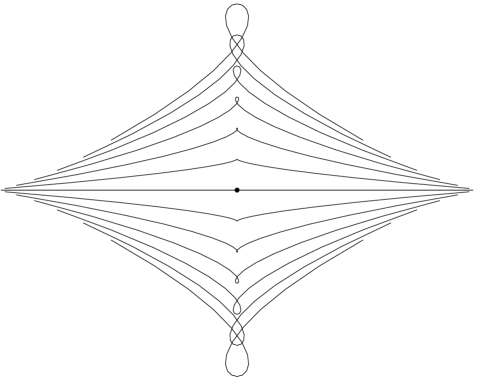
Figure 1. The generic way in which a family of open immersions crosses the hypersurface where $Z\neq\emptyset$. The parametrized straight line in the middle of the family has velocity with a double zero at the black dot, hence is not an immersion. See text.

2.4. The basic mapping in the periodic case

Next, consider the periodic cases. Here we need the Stiefel manifolds:

$$\operatorname{\bf St}(2,V)=\{\text{orthonormal pairs }(e,f)\in V\times V\},V=V_{\text{ev}}\text{ or }V_{\text{od}}$$

and $\operatorname{\bf St}^{0}(2,V)$ the subset defined by the constraint $Z(e,f)=\emptyset$. For later use, it is also convenient to note that $\operatorname{\bf St}(2,V)=\{A\in L(\mathbb{C},V):A^{T}.A=\operatorname{Id}_{\mathbb{C}}\}$ where $L(\mathbb{C},V)$ is the space of linear maps from $\mathbb{C}$ to $V$ and $\langle A^{\top}v,w\rangle_{\mathbb{C}}=\langle v,Aw\rangle_{V}$. For $(e,f)\in\operatorname{\bf S}^{0}(V^{2}_{\text{op}})$, when is $c=\Phi(e,f)$ periodic? If and only if we have:

(A) $$c^{\prime}=\tfrac{1}{2}(e+if)^{2}\quad\text{is periodic, so that }e,f\in V_{\text{ev}}\text{ or }V_{\text{od}};$$

(B) $$0=\int_{0}^{2\pi}c^{\prime}(u)\,du=\frac{1}{2}\int_{0}^{2\pi}(e^{2}-f^{2})\,du+i\int_{0}^{2\pi}ef\,du.$$

Condition B says that $\|e\|^{2}=\|f\|^{2}=1$ (since the sum is 2) and $\langle e,f\rangle=0$, so that $(e,f)\in\operatorname{\bf St}^{0}(2,V_{\text{ev}})$ or $(e,f)\in\operatorname{\bf St}^{0}(2,V_{\text{od}})$. Recall that the index $n$ of an immersed curve $c$ is defined by considering $\log(c^{\prime})$. The log must satisfy $\log(c^{\prime}(\theta+2\pi))\equiv\log(c^{\prime}(\theta))+2\pi n$ for some $n$ and this is the index. So this index is even or odd depending on whether the square root of $c^{\prime}$ is periodic or anti-periodic, that whether $(e,f)\in V_{\text{ev}}$ or $\in V_{\text{od}}$. So if $\Phi$ is restricted to $\operatorname{\bf St}^{0}(2,V_{\text{ev}})$ or $\operatorname{\bf St}^{0}(2,V_{\text{od}})$ (and is still denoted $\Phi$), it provides isometric 2-fold coverings

$$\Phi:\operatorname{\bf St}^{0}(2,V_{\text{ev}}) \longrightarrow\{c\in\operatorname{Imm}_{{\text{ev}}}(S^{1},\mathbb{C}):c(0)=0,\ell(c)=1\}$$

$$\Phi:\operatorname{\bf St}^{0}(2,V_{\text{od}}) \longrightarrow\{c\in\operatorname{Imm}_{{\text{od}}}(S^{1},\mathbb{C}):c(0)=0,\ell(c)=1\}$$

All three of these maps $\Phi$ can be modified so as to divide out by rotations. The mapping $(e,f)\mapsto e^{i\varphi}(e+if)$ produces a rotation of the immersed curve $\Phi(e,f)$ through an angle $2\varphi$. The complex projective space $\operatorname{\bf CP}(V^{2}_{\text{op}})$ is $\operatorname{\bf S}(V^{2}_{\text{op}})$ divided by the action of rotations, and we denote by $\operatorname{\bf CP}^{0}(V^{2}_{\text{op}})$ the subset gotten by dividing $\operatorname{\bf S}^{0}(V^{2}_{\text{op}})$ by rotations. The group generated by translations, rotations and scalings will be called the group of similitudes, abreviated as ‘sim’. Then we get the variant:

$$\Phi:\operatorname{\bf CP}^{0}(V^{2}_{\text{op}})\longrightarrow\operatorname{Imm}_{\text{op}}/(\text{sim}).$$

Similarly, let $\operatorname{\bf Gr}(2,V)$ be the Grassmannian of unoriented 2-dimensional subspaces of $V$ and let $\operatorname{\bf Gr}^{0}(2,V)$ be the subset of those $W$ with $Z(W)=\emptyset$ for $V=V_{\text{ev}}$ or $=V_{\text{od}}$. Then we have maps:

$$\Phi:\operatorname{\bf Gr}^{0}(2,V_{\text{ev}}) \longrightarrow\operatorname{Imm}_{{\text{ev}}}/(\text{sim})$$

$$\Phi:\operatorname{\bf Gr}^{0}(2,V_{\text{od}}) \longrightarrow\operatorname{Imm}_{{\text{od}}}/(\text{sim})$$

For later use, we describe the tangent spaces of these spaces. The tangent space $T_{W}\operatorname{\bf Gr}$ to $\operatorname{\bf Gr}(2,V)$ at $W\in\operatorname{\bf Gr}(2,V)$ is naturally identified with $L(W,W^{\bot})$ and has the following norm, induced from that on $V$:

$$\|v\|^{2}=\text{tr}(v^{T}\circ v)=\|v(e)\|^{2}+\|v(f)\|^{2}$$

for $v\in T_{W}\operatorname{\bf Gr}$ and $\{e,f\}$ an orthonormal basis of $W$. Similarly, $T_{(e,f)}\operatorname{\bf St}$ can be naturally identified with pairs $\{\delta e,\delta f\}$ in $V$ such that $\langle e,\delta e\rangle=\langle f,\delta f\rangle=\langle e,\delta f\rangle+\langle f,\delta e\rangle=0$ with norm:

$$\|(\delta e,\delta f)\|^{2}=\|\delta e\|^{2}+\|\delta f\|^{2}.$$

The same definition holds for $T_{(e,f)}(\operatorname{\bf S})$, this time with the constraint $\langle e,\delta e\rangle+\langle f,\delta f\rangle=0$.

3. The Basic Mapping for Shapes

3.1. Dividing out by the group of reparametrizations

Let $C^{\infty,+}([0,2\pi])$ be the group of increasing diffeomorphisms $\varphi$ of $[0,2\pi]$ (so $\varphi(0)=0,\varphi(2\pi)=2\pi$) and let $C^{\infty,+}(\mathbb{R})$ be the group of increasing $C^{\infty}$ diffeomorphisms $\varphi:\mathbb{R}\rightarrow\mathbb{R}$ such that $\varphi(x+2\pi)\equiv\varphi(x)+2\pi$ for all $x$. Modulo the central subgroup of translations $\varphi(x)=x+2\pi n$, the second group is just $\operatorname{\bf Diff}^{+}(S^{1})$. For $V=V_{\text{op}},V_{\text{ev}},V_{\text{od}}$ let $U(V)$ be the group of unitary maps on $V$ given by:

$$f\mapsto f^{\varphi}=\sqrt{\varphi^{\prime}}.(f\circ\varphi),\text{ where }\left\{\begin{array}[]{l}\varphi\in C^{\infty,+}([0,2\pi])\text{ if }V=V_{\text{op}}\\ \varphi\in C^{\infty,+}(\mathbb{R})\text{ if }V=V_{{\text{ev}}},V_{{\text{od}}}\end{array}\right.$$

These are the reparametrization groups for our various spaces. The infinitesimal action of a vector field $X$ on $[0,2\pi]$ or a periodic vector field $X$ on $S^{1}$ is then

(3) $$f\mapsto\tfrac{1}{2}X_{\theta}.f+X.f_{\theta}.$$

For all three sets of isometries $\Phi$, we can now divide each side by the reparametrization group $U(V)$. For open curves, we get a diagram

and a similar one for closed curves of even and odd index where $V=V_{\text{ev}},V_{\text{od}}$ and $B=B_{i,{\text{ev}}},B_{i,od}$:

Here we have divided by isometries on both the left and right: by $U(V)$ or $U(V)\times S^{1}$ on the left (where $S^{1}$ rotates the basis $\{e,f\}$) and by reparametrizations and rotations on the right. Thus $\overline{\Phi}$ is again an isometry if we make both quotients into Riemannian submersions. This means we must identify the tangent spaces to the quotients with the horizontal subspaces of the tangent spaces in the larger space, i.e. those perpendicular to the orbits of the isometric group actions. For $\operatorname{\bf St}$, this means:

3.2 Proposition.

The tangent vector $\{\delta e,\delta f\}$ to $\operatorname{\bf St}$ satisfies:

$$\langle\delta e,e\rangle=\langle\delta f,f\rangle=0,\langle\delta e,f\rangle+\langle\delta f,e\rangle=0.$$

It is horizontal for the rotation action if and only if:

$$\text{both }\delta e,\delta f\text{ are perpendicular to both }e,f.$$

It is horizontal for the reparametrization group if:

$$W_{\theta}(e,\delta e)+W_{\theta}(f,\delta f)=0$$

where $W_{\theta}(a,b)=a.b_{\theta}-b.a_{\theta}$ is the Wronskian with respect to the parameter $\theta$.

Proof. Consider the action of rotations, which is one-dimensional, with orbits $\beta\mapsto e^{i\beta}(e+if)$; the direction at $(e,f)$ is chosen as $(-f,e)$. So $(\delta e,\delta f)$ being horizontal at $(e,f)$ for this action means that $-\langle f,\delta e\rangle+\langle e,\delta f\rangle=0$. This proves the first assertion.

For the action of $U(V)$, one has to note that horizontal vectors must satisfy

$$\langle\tfrac{1}{2}X_{\theta}.e+X.e_{\theta},\delta e\rangle+\langle\tfrac{1}{2}X_{\theta}.f+X.f_{\theta},\delta f\rangle=0$$

for any periodic vector field $X$ on $\mathbb{R}$, which yields the horizontality condition after integration by parts of the terms in $X_{\theta}$. ∎

Horizontality on the shape space side means (see [11]):

3.3 Proposition.

$h\in T_{c}\operatorname{Imm}(S^{1},\mathbb{C})$ is horizontal for the action of $\operatorname{Diff}(S^{1})$ if and only if $D_{s}^{2}(h)$ is normal to the curve, i.e. $\langle v,D_{s}^{2}(h)\rangle=0$.

3.4 Proposition.

For any smooth path $c$ in $\operatorname{Imm}(S^{1},\mathbb{R}^{2})$ there exists a smooth path $\varphi$ in $\operatorname{Diff}(S^{1})$ with $\varphi(0,\;.\;)=\operatorname{Id}_{S^{1}}$ depending smoothly on $c$ such that the path $e$ given by $e(t,\theta)=c(t,\varphi(t,\theta))$ is horizontal: $\langle D_{s}^{2}(e_{t}),e_{\theta}\rangle=0$.

This is a variant of [11, 4.6].

Proof. Writing $D_{c}$ instead of $D_{s}$ we note that $D_{c\circ\varphi}(f\circ\varphi)=\frac{(f_{\theta}\circ\varphi)\varphi_{\theta}}{|c_{\theta}\circ\varphi|.|\varphi_{\theta}|}=(D_{c}(f))\circ\varphi$ for $\varphi\in\operatorname{Diff}^{+}(S^{1})$. So we have $L_{n,c\circ\varphi}(f\circ\varphi)=(L_{n,c}f)\circ\varphi$.

Let us write $e=c\circ\varphi$ for $e(t,\theta)=c(t,\varphi(t,\theta))$, etc. We look for $\varphi$ as the integral curve of a time dependent vector field $\xi(t,\theta)$ on $S^{1}$, given by $\varphi_{t}=\xi\circ\varphi$. We want the following expression to vanish:

$$\langle D_{c\circ\varphi}^{2}(\partial_{t}(c\circ\varphi)),\partial_{\theta}(c\circ\varphi)\rangle =\langle D_{c\circ\varphi}^{2}(c_{t}\circ\varphi+(c_{\theta}\circ\varphi)\,\varphi_{t}),(c_{\theta}\circ\varphi)\,\varphi_{\theta}\rangle$$

$$=\langle D_{c}^{2}(c_{t})\circ\varphi+D_{c}^{2}(c_{\theta}.\xi)\circ\varphi,c_{\theta}\circ\varphi\rangle\varphi_{\theta}$$

$$=\bigl{(}(\langle D_{c}^{2}(c_{t}),c_{\theta}\rangle+\langle D_{c}^{2}(\xi.c_{\theta}),c_{\theta}\rangle)\circ\varphi\bigr{)}\,\varphi_{\theta}.$$

Using the time dependent vector field $\xi=-\frac{1}{|c_{\theta}|}D_{c}^{-2}(\langle D_{c}^{2}(c_{t}),v\rangle)$ and its flow $\varphi$ achieves this. ∎

3.5. Bigger spaces

As we will see below, we can describe geodesics in the ‘classical’ spaces $\operatorname{\bf S},\operatorname{\bf CP},\operatorname{\bf St},\operatorname{\bf Gr}$ quite explicitly. By the above isometries, this gives us the geodesics in the various spaces $\operatorname{Imm},B_{i}$. BUT, as we mentioned above for the space $\operatorname{\bf S}$, geodesics in the ‘good’ parts $\operatorname{\bf S}^{0},\operatorname{\bf CP}^{0},\operatorname{\bf St}^{0},\operatorname{\bf Gr}^{0}$ do not stay there, but they cross the ‘bad’ part where $Z(e,f)\neq\emptyset$. Now the basic mapping is still defined on the full sphere, projective space, Stiefel manifold or Grassmannian, giving us some smooth mappings of $[0,2\pi]$ or $S^{1}$ to $\mathbb{C}$, possibly modulo translations, rotations and/or scalings.

But when we divide by $U(V_{\text{op}})$, a major problem arises. The orbits of $U(V_{\text{op}})$ acting on $C^{\infty}([0,2\pi],\mathbb{C})$ are not closed, hence the topological quotient of the space $C^{\infty}([0,2\pi],\mathbb{C})$ by $U(V_{\text{op}})$ is not Hausdorff. This is shown by the following construction:

1. Start with a $C^{\infty}$ non-decreasing map $\psi$ from $[0,2\pi]$ to itself such that $\psi(\theta)\equiv\pi$ for $\theta$ in some interval $I$.

2. Let $\psi_{n}(\theta)=(1-1/n).\psi(\theta)+\theta/n$. The sequence $\{\psi_{n}\}$ of diffeomorphisms of $[0,2\pi]$ converges to $\psi$.

3. Then for any $c\in\operatorname{Imm}_{\text{op}}$, the maps $c\circ\psi_{n}$ are all in the orbit of $c$. But they converge to $c\circ\psi$ which is constant on the whole interval $I$, hence is not in the orbit.

Thus, if we want some Hausdorff space of curves which a) have singularities more complex than those of immersed curves and b) can hold the extensions of geodesics in some space $B_{i}$ which come from the map $\Phi$, we must divide $C^{\infty}([0,2\pi],\mathbb{C})$ by some equivalence relation larger than the group action by $U(V)$. The simplest seems to be: first define a monotone relation $R\subset[0,2\pi]\times[0,2\pi]$ to be any closed subset such that $p_{1}(R)=p_{2}(R)=[0,2\pi]$ ($p_{1}$ and $p_{2}$ being the projections on the axes) and for every pair of points $(s_{1},t_{1})\in R$ and $(s_{2},t_{2})\in R$, either $s_{1}\leq s_{2}$ and $t_{1}\leq t_{2}$ or vice versa. Then $f,g:[0,2\pi]\rightarrow\mathbb{C}$ are Fréchet equivalent if there is a monotone relation $R$ such that $f(s)=g(t),\forall(s,t)\in R$.

This is a good equivalence relation because if $\{f_{n}\},\{g_{n}\}:[0,2\pi]\rightarrow\mathbb{C}$ are two sequences and $\lim_{n}f_{n}=f,\lim_{n}g_{n}=g$ and $f_{n},g_{n}$ are Fréchet equivalent for all $n$, then $f,g$ are Fréchet equivalent. The essential point is that the set of non-empty closed subsets of a compact metric space $X$ is compact in the Hausdorff topology (see [1]). Thus if $\{R_{n}\}$ are the monotone relations instantiating the equivalence of $f_{n}$ and $g_{n}$, a subsequence $\{R_{n_{k}}\}$ Hausdorff converges to some $R\subset[0,2\pi]\times[0,2\pi]$ and it is immediate that $R$ is a monotone relation making $f$ and $g$ Fréchet equivalent.

Define

$$B_{\text{big},\text{op}}=C^{\infty}([0,2\pi],\mathbb{C})/\text{Fr\'{e}chet equivalence, translations, scalings}.$$

Then we have a commutative diagram:

Thus the whole of a geodesic which enters the ‘bad’ part of $\operatorname{\bf S}(V_{\text{op}})$ creates a path in $B_{big,\text{op}}$. Of course, the same construction works for closed curves also. We will see several examples in the next section.

4. Construction of Geodesics

4.1. Great circles in Spheres

The space $\operatorname{\bf S}(V^{2})$ being the sphere of radius $\sqrt{2}$ on $V^{2}$, its geodesics are the great circles. Thus, the geodesic distance between $(e^{0},f^{0})$ and $(e^{1},f^{1})$ is given by $\sqrt{2}D$ with

$$D=\arccos\big{(}({\left\langle{e^{0}}\,,\,{e^{1}}\right\rangle}+{\left\langle{f^{0}}\,,\,{f^{1}}\right\rangle})/2\big{)}$$

and the geodesic is given by

$$e(t) = \frac{\sin((1-t)D)}{\sin D}e^{0}+\frac{\sin(tD)}{\sin D}e^{1}$$

$$f(t) = \frac{\sin((1-t)D)}{\sin D}f^{0}+\frac{\sin(tD)}{\sin D}f^{1}$$

The corresponding geodesic on $\operatorname{Imm}_{\text{op}}$ modulo translation and scaling is the time-indexed family of curves $t\mapsto c(u,t)$ with

$$\partial c/\partial u=\tfrac{1}{2}(e(t)+if(t))^{2}=(e(t)^{2}-f(t)^{2})/2+ie(t)f(t)$$

The following notation will be used throughout this section:

$$c^{0}(u) =c(u,0), c^{1}(u) =c(u,1)$$

$$\partial c^{0}/\partial u =r_{0}(u)e^{i\alpha^{0}(u)}, \partial c^{1}/\partial u =r_{1}(u)e^{i\alpha^{1}(u)}$$

so that $e^{j}=\sqrt{2r_{j}}\cos\tfrac{\alpha^{j}}{2}$ and $f^{j}=\sqrt{2r_{j}}\sin\tfrac{\alpha^{j}}{2}$ for $j=0,1$. Thus the distance $D$ is

$$D_{\text{op}}(c^{0},c^{1})=\arccos\int_{0}^{2\pi}\sqrt{r_{0}r_{1}}\cos\frac{\alpha^{1}-\alpha^{0}}{2}du.$$

The metric on $\operatorname{Imm}_{\text{op}}$ modulo rotations is

$$D_{\text{op, rot}}(c^{0},c^{1})=\inf_{\alpha}\arccos\int_{0}^{2\pi}\sqrt{r_{0}r_{1}}\cos\frac{\alpha^{1}-\alpha^{0}-\alpha}{2}du$$

$$=\arccos\sup_{\alpha}\int_{0}^{2\pi}\sqrt{r_{0}r_{1}}\left(\cos\frac{\alpha^{1}-\alpha^{0}}{2}\cos\frac{\alpha}{2}+\sin\frac{\alpha^{1}-\alpha^{0}}{2}\sin\frac{\alpha}{2}\right)du$$

$$=\arccos\left(\Big{(}\int_{0}^{2\pi}\sqrt{r_{0}r_{1}}\cos\frac{\alpha^{1}-\alpha^{0}}{2}du\Big{)}^{2}+\Big{(}\int_{0}^{2\pi}\sqrt{r_{0}r_{1}}\sin\frac{\alpha^{1}-\alpha^{0}}{2}du\Big{)}^{2}\right)^{1/2}$$

The distance on $B_{i,\text{op}}$ is the infimum of this expression over all changes of coordinate for $c^{0}$. Assuming that $c^{0}$ and $c^{1}$ are originally parametrized with $1/2\pi$ times arc-length so that $r_{0}\equiv 1/2\pi,r_{1}\equiv 1/2\pi$, this is

(4) $$D_{\text{op, diff}}(c^{0},c^{1})=\arccos\sup_{\phi}\frac{1}{2\pi}\int_{0}^{2\pi}\sqrt{\phi_{\theta}}\cos\frac{\alpha^{1}\circ\phi-\alpha^{0}}{2}d\theta$$

and modulo rotations

$$D_{\text{op, diff, rot}}(c^{0},c^{1})=\arccos\sup_{\phi}\left(\Big{(}\frac{1}{2\pi}\int_{0}^{2\pi}\sqrt{\phi_{\theta}}\cos\frac{\alpha^{1}\circ\phi-\alpha^{0}}{2}d\theta\Big{)}^{2}\right.\\ \left.+\Big{(}\frac{1}{2\pi}\int_{0}^{2\pi}\sqrt{\phi_{\theta}}\sin\frac{\alpha^{1}\circ\phi-\alpha^{0}}{2}d\theta\Big{)}^{2}\right)^{1/2}.$$

The supremum in both expressions is taken over all increasing bijections $\phi\in C^{\infty}([0,2\pi],[0,2\pi])$.

To shorten these formulae, we will use the following notation. Define:

$$C_{-}(\phi) =\frac{1}{2\pi}\int_{0}^{2\pi}\sqrt{\phi_{\theta}}\cos\frac{\alpha^{1}\circ\phi-\alpha^{0}}{2}d\theta$$

$$S_{-}(\phi) =\frac{1}{2\pi}\int_{0}^{2\pi}\sqrt{\phi_{\theta}}\sin\frac{\alpha^{1}\circ\phi-\alpha^{0}}{2}d\theta$$

Then we have:

$$D_{\text{op, diff}} =\inf_{\phi}\arccos(C_{-}(\phi))\quad\text{ and}$$

$$D_{\text{op, diff, rot}} =\inf_{\phi}\arccos\big{(}\sqrt{(C_{-}(\phi))^{2}+(S_{-}(\phi))^{2}}\big{)}.$$

4.2. Problems with the existence of geodesics

These expressions give very explicit descriptions of distance and geodesics. We have already noted, however, that, even if both $(e^{0},f^{0})$ and $(e^{1},f^{1})$ belong to $\operatorname{\bf S}^{0}$, the same property is not guaranteed at each point of the geodesic. $e(\alpha,t)=f(\alpha,t)=0$ happens for some $t$ whenever $(e^{0}(\alpha),f^{0}(\alpha))$ and $(e^{1}(\alpha),f^{1}(\alpha))$ are collinear with opposite orientations. This is not likely to happen for geodesics joining nearby points. When it does happen, it is usually a stable phenomenon: for example, if the geodesic crosses $\operatorname{\bf S}-\operatorname{\bf S}^{0}$ transversally, as illustrated in figure 1, then this happens for all nearby geodesics too. Note that this means that the geodesic spray on $\operatorname{Imm}_{\text{op}}$ is not surjective. In fact, any geodesic on $\operatorname{Imm}_{\text{op}}$ comes from a great circle on $\operatorname{\bf S}^{0}$ and if it crosses $\operatorname{\bf S}-\operatorname{\bf S}^{0}$, it leaves $\operatorname{Imm}_{\text{op}}$.

When we pass to the quotient by reparametrizations, another question arises: does the inf over reparametrizations exist? or equivalently is there is a horizontal geodesic joining any two open curves? In fact, there need not be any such geodesic even if you allow it to cross $\operatorname{\bf S}-\operatorname{\bf S}^{0}$. In general, to obtain a geodesic minimizing distance between 2 open curves, the curves themselves must be given parametrizations with zero velocity somewhere, i.e. they may need to be lifted to points in $\operatorname{\bf S}-\operatorname{\bf S}^{0}$.

This is best illustrated by the special case in which $c^{1}$ is the line segment from $0$ to $1$, namely $e^{1}+if^{1}=1/\sqrt{\pi}$, $\alpha^{1}\equiv 0$. The curve $c^{0}$ can be arbitrary. Then the reparametrization $\phi$ which minimizes distance is the one which maximizes:

$$\int_{0}^{2\pi}\sqrt{\phi_{\theta}}\cos\frac{\alpha^{0}}{2}d\theta.$$

This variational problem is easy to solve: the optimal $\phi$ is given by:

$$\phi(u)=2\pi\int_{0}^{u}\max\left(\cos\frac{\alpha^{0}}{2},0\right)^{2}\Bigg{/}\int_{0}^{2\pi}\max\left(\cos\frac{\alpha^{0}}{2},0\right)^{2}.$$

Note that $\phi$ is not in general a diffeomorphism: it is constant on intervals where $\cos(\alpha^{0}/2)\leq 0$. Its graph is a monotone relation in the sense of section 3.5. In fact, it’s easy to see that monotone relations enjoy a certain compactness, so that the inf over reparametrizations is always achieved by a monotone relation. Assuming $\alpha^{0}$ is represented by a continuous function for which $-2\pi<\alpha^{0}(u)<2\pi$, the result is that the places on the curve $c^{0}$ where $|\alpha^{0}(u)|>\pi$ get squashed to points on the line segment. The result is that this limit geodesic is not actually a path in the space $B$ of smooth curves. Figure 2 illustrates this effect.

The general problem of maximizing the functional

$$U(\phi)=\frac{1}{2\pi}\int_{0}^{2\pi}\sqrt{\phi_{\theta}}\cos\frac{\alpha^{1}\circ\phi-\alpha^{0}}{2}d\theta$$

with respect to increasing functions $\phi$ has been addressed in [17]. Existence of solutions can be shown in the class of monotone relations, or, equivalently functions $\phi$ that take the form $\phi(s)=\mu([0,s))$ for some positive measure $\mu$ on $[0,2\pi]$ with total mass less or equal to $2\pi$ ($\phi_{\theta}$ being replaced by the Radon-Nykodim derivative of $\mu$ in the definition of $U$). The optimal $\phi$ is a diffeomorphism as soon as $\cos((\alpha^{1}(u)-\alpha^{0}(v))/{2})>0$ whenever $|u-v|$ is smaller than a constant (which depends on $\alpha^{0}$ and $\alpha^{1}$). More details can be found in [17].

It is easy to show that maximizing $U$ is equivalent to maximizing

$$U^{+}(\phi)=\frac{1}{2\pi}\int_{0}^{2\pi}\sqrt{\phi_{\theta}}\max\left(\cos\frac{\alpha^{1}\circ\phi-\alpha^{0}}{2},0\right)d\theta$$

because one can always modify $\phi$ on intervals on which $\cos((\alpha^{1}\circ\phi-\alpha^{0})/{2})<0$ to ensure that $\phi_{\theta}d\theta=0$. In [18], it is proposed to maximize

$$\bar{U}(\phi)=\frac{1}{2\pi}\int_{0}^{2\pi}\sqrt{\phi_{\theta}}\left|\cos\frac{\alpha^{1}\circ\phi-\alpha^{0}}{2}\right|d\theta.$$

This corresponds to replacing the lift $e(u)+if(u)$ by $\sigma(u).(e(u)+if(u))$ where $\sigma(u)=\pm$ for all $u$, but this is beyond the scope of this paper.

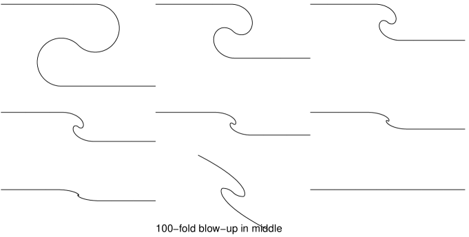
Figure 2. This is a geodesic of open curves running from the curve with the kink at the top left to the straight line on the bottom right. A blow up of the next to last curve is shown to reveal that the kink never goes away – it merely shrinks. Thus this geodesic is not continuous in the $C^{1}$-topology on $B_{\text{op}}$. The straight line is parametrized so that it stops for a whole interval of time when it hits the middle point and thus it is $C^{1}$-continuous in $\operatorname{Imm}_{\text{op}}$.

4.3. Neretin geodesics on $\operatorname{\bf Gr}(2,V)$

The integrated path-length distance and explicit geodesics can be found in any Grassmannian using Jordan Angles [13] as follows: If $W_{0},W_{1}\subset V$ are two 2-dimensional subspaces the singular value decomposition of the orthogonal projection $p$ of $W_{0}$ to $W_{1}$ gives orthonormal bases $\{e^{0},f^{0}\}$ of $W_{0}$ and $\{e^{1},f^{1}\}$ of $W_{1}$ such that $p(e^{0})=\lambda_{e}.e^{1}$, $p(f^{0})=\lambda_{f}f^{1}$, $e^{0}\perp f^{1}$ and $f^{0}\perp e^{1}$, where $0\leq\lambda_{f},\lambda_{e}\leq 1$. Write $\lambda_{e}=\cos(\psi_{e}),\lambda_{f}=\cos(\psi_{f})$ then $\psi_{e}$, $\psi_{f}$ are the Jordan angles, $0\leq\psi_{e},\psi_{f}\leq\pi/2$. The global metric is given by:

$$d(W^{0},W^{1})=\sqrt{\psi_{e}^{2}+\psi_{f}^{2}}$$

and the geodesic by:

(5) $$W(t)=\left\{{\begin{aligned} e(t)&=\frac{\sin((1-t).\psi_{e})e^{0}+\sin(t\psi_{e})e^{1}}{\sin\psi_{e}},\\ f(t)&=\frac{\sin((1-t).\psi_{f})f^{0}+\sin(t\psi_{f})f^{1}}{\sin\psi_{f}}\end{aligned}}\right\}.$$

We apply this now in order to compute the distance between the curves in the two spaces $\operatorname{Imm}_{{\text{ev}}}/(\text{sim})$ and $\operatorname{Imm}_{{\text{od}}}/(\text{sim})$, as well as in the unparametrized quotients $B_{i,{\text{ev}}}/(\text{sim})$ and $B_{i,{\text{od}}}/(\text{sim})$. We write as above $\partial_{\theta}c^{0}=r_{0}(\theta)e^{i\alpha^{0}(\theta)}$ and $\partial_{\theta}c^{1}=r_{1}(\theta)e^{i\alpha^{1}(\theta)}$. We put

$$\bar{e}^{0} =\sqrt{2r_{0}}\cos\tfrac{\alpha^{0}}{2} \quad\bar{f}^{0} =\sqrt{2r_{0}}\sin\tfrac{\alpha^{0}}{2},$$

$$\bar{e}^{1} =\sqrt{2r_{1}}\cos\tfrac{\alpha^{1}}{2} \quad\bar{f}^{1} =\sqrt{2r_{1}}\sin\tfrac{\alpha^{1}}{2}$$

thus lifting these curves to 2-planes in the Grassmannian. The $2\times 2$ matrix of the orthogonal projection from the space $\{\bar{e}^{0},\bar{f}^{0}\}$ to $\{\bar{e}^{1},\bar{f}^{1}\}$ in these bases is:

$$M(c^{0},c^{1})=\begin{pmatrix}\int_{S^{1}}2\sqrt{r^{0}.r^{1}}.\cos\tfrac{\alpha^{0}}{2}\cos\tfrac{\alpha^{1}}{2}\,d\theta&\int_{S^{1}}2\sqrt{r^{0}.r^{1}}.\cos\tfrac{\alpha^{0}}{2}\sin\tfrac{\alpha^{1}}{2}\,d\theta\\ \\ \int_{S^{1}}2\sqrt{r^{0}.r^{1}}.\sin\tfrac{\alpha^{0}}{2}\cos\tfrac{\alpha^{1}}{2}\,d\theta&\int_{S^{1}}2\sqrt{r^{0}.r^{1}}.\sin\tfrac{\alpha^{0}}{2}\sin\tfrac{\alpha^{1}}{2}\,d\theta\end{pmatrix}$$

It will be convenient to use the notations:

$$C_{\pm} :=\int_{S^{1}}\sqrt{r^{0}.r^{1}}\cos\tfrac{\alpha^{0}\pm\alpha^{1}}{2}\,d\theta=\tfrac{1}{2}\left(M(c^{0},c^{1})_{11})\mp M(c^{0},c^{1})_{22}\right)$$

$$S_{\pm} :=\int_{S^{1}}\sqrt{r^{0}.r^{1}}\sin\tfrac{\alpha^{0}\pm\alpha^{1}}{2}\,d\theta=\tfrac{1}{2}\left(M(c^{0},c^{1})_{21}\pm M(c^{0},c^{1})_{12}\right)$$

We have to diagonalize this matrix by rotating the curve $c^{0}$ by a constant angle $\beta^{0}$, i.e., the basis $\{\bar{e}^{0},\bar{f}^{0}\}$ by the angle $\beta^{0}/2$; and similarly the curve $c^{1}$ by a constant angle $\beta^{1}$. So we have to replace $\alpha^{0}$ by $\alpha^{0}-\beta^{0}$ and $\alpha^{1}$ by $\alpha^{1}-\beta^{1}$ in such a way that

(6) $$0 =\int_{S^{1}}\sqrt{r^{0}.r^{1}}\sin\left(\frac{(\alpha^{0}-\beta^{0})\pm(\alpha^{1}-\beta^{1})}{2}\right)d\theta\quad\text{ (for both signs)}$$

$$=S_{\pm}.\cos\tfrac{\beta^{0}\pm\beta^{1}}{2}-C_{\pm}.\sin\tfrac{\beta^{0}\pm\beta^{1}}{2}$$

Thus

$$\beta_{0}\pm\beta_{1}=2\arctan\left(S_{\pm}/C_{\pm}\right).$$

In the newly aligned bases, the diagonal elements of $M(c^{0},c^{1})$ will be the cosines of the Jordan angles. But even without preliminary diagonalization, the following lemma gives you a formula for them:

Lemma.

If $M=\left(\begin{array}[]{cc}a&b\\ c&d\end{array}\right)$ and $C_{\pm}=\tfrac{1}{2}(a\mp d),S_{\pm}=\tfrac{1}{2}(c\pm b)$, then the singular values of $M$ are:

$$\sqrt{C_{-}^{2}+S_{-}^{2}}\pm\sqrt{C_{+}^{2}+S_{+}^{2}}.$$

The proof is straightforward. This gives the formula

(7) $$D_{{\text{od}},\text{rot}}(c^{0},c^{1})^{2}= \arccos^{2}\Big{(}\sqrt{S_{+}^{2}+C_{+}^{2}}+\sqrt{S_{-}^{2}+C_{-}^{2}}\Big{)}$$

$$+ \arccos^{2}\Big{(}\sqrt{S_{-}^{2}+C_{-}^{2}}-\sqrt{S_{+}^{2}+C_{+}^{2}}\Big{)}.$$

This is the distance in the space $\operatorname{Imm}_{{\text{od}}}(S^{1},\mathbb{C})$/(transl, rot., scalings).

4.4. Horizontal Neretin distances

If we want the distance in the quotient space $B_{i,{\text{od}}}/(\text{transl, rot., scalings})$ by the group $\text{Diff}(S^{1})$ we have to take the infimum of 7 over all reparametrizations. To simplify the formulas that follow, we can assume that the initial curves $c^{0},c^{1}$ are parametrized by arc length so that $r^{0}\equiv r^{1}\equiv 1/2\pi$. Then consider a reparametrization $\phi\in\text{Diff}(S^{1})$ of one of the two curves, say $c^{0}\circ\phi$:

(8) $$D_{\text{sim,diff}}(c^{0},c^{1})^{2}=\inf_{\phi}\left(\arccos^{2}(\lambda_{e}(c^{0}\circ\phi,c^{1}))+\arccos^{2}(\lambda_{f}(c^{0}\circ\phi,c^{1}))\right)$$

where now

$$\lambda_{e}(c^{0}\circ\phi,c^{1}) =\sqrt{S_{-}^{2}(\phi)+C_{-}^{2}(\phi)}+\sqrt{S_{+}^{2}(\phi)+C_{+}^{2}(\phi)}$$

$$\lambda_{f}(c^{0}\circ\phi,c^{1}) =\sqrt{S_{-}^{2}(\phi)+C_{-}^{2}(\phi)}-\sqrt{S_{+}^{2}(\phi)+C_{+}^{2}(\phi)}$$

$$S_{\pm}(\phi) :=\frac{1}{2\pi}\int_{S^{1}}\sqrt{\phi_{\theta}}\sin\tfrac{(\alpha^{0}\circ\phi)\pm\alpha^{1}}{2}\,d\theta,$$

$$C_{\pm}(\phi) :=\frac{1}{2\pi}\int_{S^{1}}\sqrt{\phi_{\theta}}\cos\tfrac{(\alpha^{0}\circ\phi)\pm\alpha^{1}}{2}\,d\theta.$$

To describe the inf, we can use the fact that geodesics on the space of curves are the horizontal geodesics in the space of immersions. Consider the geodesic $t\mapsto\{e(t),f(t)\}$ in $\operatorname{\bf Gr}(2,V)$ described in 5, for

$$e^{0} =\sqrt{\tfrac{\phi_{\theta}}{\pi}}\cos\tfrac{(\alpha^{0}\circ\phi)-\beta^{0}}{2} \quad e^{1} =\tfrac{1}{\sqrt{\pi}}\cos\tfrac{\alpha^{1}-\beta^{1}}{2},$$

$$f^{0} =\sqrt{\tfrac{\phi_{\theta}}{\pi}}\sin\tfrac{(\alpha^{0}\circ\phi)-\beta^{0}}{2} \quad f^{1} =\tfrac{1}{\sqrt{\pi}}\sin\tfrac{\alpha^{1}-\beta^{1}}{2},$$

where the rotations $\beta^{0}$ and $\beta^{1}$ must be computed from $c^{0}\circ\phi$ and $c^{1}$. Note that

$$e^{0}_{\theta} =\frac{\phi_{\theta\theta}}{2\sqrt{\pi\phi_{\theta}}}\cos\tfrac{(\alpha^{0}\circ\phi)-\beta^{0}}{2}-\tfrac{1}{2\sqrt{\pi}}\phi_{\theta}^{3/2}.(\alpha^{0}_{\theta}\circ\phi).\sin\tfrac{(\alpha^{0}\circ\phi)-\beta^{0}}{2};$$

$$e^{1}_{\theta} =\tfrac{-1}{2\sqrt{\pi}}.\alpha^{1}_{\theta}.\sin\tfrac{\alpha^{1}-\beta^{1}}{2}$$

$$f^{0}_{\theta} =\frac{\phi_{\theta\theta}}{2\sqrt{\pi\phi_{\theta}}}\sin\tfrac{(\alpha^{0}\circ\phi)-\beta^{0}}{2}+\tfrac{1}{2\sqrt{\pi}}\phi_{\theta}^{3/2}.(\alpha^{0}_{\theta}\circ\phi).\cos\tfrac{(\alpha^{0}\circ\phi)-\beta^{0}}{2};$$

$$f^{1}_{\theta} =\tfrac{1}{2\sqrt{\pi}}.\alpha^{1}_{\theta}.\cos\tfrac{\alpha^{1}-\beta^{1}}{2}$$

If the Jordan angles are $\psi_{e}$ and $\psi_{f}$, then the tangent vector to the geodesic $t\mapsto W(t)$ at $t=0$ is described by

$$e_{t}(0)=\partial_{t}|_{0}e=\frac{\psi_{e}}{\sin\psi_{e}}.\left(e^{1}-\cos\psi_{e}.e^{0}\right),\;\;f_{t}(0)=\partial_{t}|_{0}f=\frac{\psi_{f}}{\sin\psi_{f}}.\left(f^{1}-\cos\psi_{f}.f^{0}\right)$$

By 3.2 the geodesic is perpendicular to all $\operatorname{Diff}(S^{1})$-orbits if and only if the sum of Wronskians vanishes:

$$0=W_{\theta}(e^{0},e_{t}(0))+W_{\theta}(f^{0},f_{t}(0))=$$

$$=e^{0}\frac{\psi_{e}}{\sin\psi_{e}}\left(e^{1}_{\theta}-\cos\psi_{e}e^{0}_{\theta}\right)-e^{0}_{\theta}\frac{\psi_{e}}{\sin\psi_{e}}\left(e^{1}-\cos\psi_{e}e^{0}\right)$$

$$\quad+f^{0}\frac{\psi_{f}}{\sin\psi_{f}}\left(f^{1}_{\theta}-\cos\psi_{f}f^{0}_{\theta}\right)-f^{0}_{\theta}\frac{\psi_{f}}{\sin\psi_{f}}\left(f^{1}-\cos\psi_{f}f^{0}\right)$$

$$=\frac{\psi_{e}}{\sin\psi_{e}}W_{\theta}(e^{0},e^{1})+\frac{\psi_{f}}{\sin\psi_{f}}W_{\theta}(f^{0},f^{1})$$

$$=-\frac{1}{\sqrt{\phi_{\theta}}}\Big{\{}\phi_{\theta\theta}\Big{(}\frac{\psi_{e}}{\sin\psi_{e}}\cos\tfrac{(\alpha^{0}\circ\phi)-\beta^{0}}{2}\cos\tfrac{\alpha^{1}-\beta^{1}}{2}+\frac{\psi_{f}}{\sin\psi_{f}}\sin\tfrac{(\alpha^{0}\circ\phi)-\beta^{0}}{2}\sin\tfrac{\alpha^{1}-\beta^{1}}{2}\Big{)}$$

$$\quad-\phi_{\theta}\alpha^{1}_{\theta}\Big{(}\frac{\psi_{e}}{\sin\psi_{e}}\cos\tfrac{(\alpha^{0}\circ\phi)-\beta^{0}}{2}\sin\tfrac{\alpha^{1}-\beta^{1}}{2}-\frac{\psi_{f}}{\sin\psi_{f}}\sin\tfrac{(\alpha^{0}\circ\phi)-\beta^{0}}{2}\cos\tfrac{\alpha^{1}-\beta^{1}}{2}\Big{)}$$

$$\quad+\phi_{\theta}^{2}(\alpha^{0}_{\theta}\circ\phi)\Big{(}\frac{\psi_{e}}{\sin\psi_{e}}\sin\tfrac{(\alpha^{0}\circ\phi)-\beta^{0}}{2}\cos\tfrac{\alpha^{1}-\beta^{1}}{2}-\frac{\psi_{f}}{\sin\psi_{f}}\cos\tfrac{(\alpha^{0}\circ\phi)-\beta^{0}}{2}\sin\tfrac{\alpha^{1}-\beta^{1}}{2}\Big{)}\Big{\}}$$

This is an ordinary differential equation for $\phi$ which is coupled to the (integral) equations for calculating the $\beta$’s as functions of $\phi$. If it is non-singular (i.e., the coefficient function of $\phi_{\theta\theta}$ does not vanish for any $\theta$) then there is a solution $\phi$, at least locally. But the non-existence of the inf described for open curves above will also affect closed curves and global solutions may actually not exist. However, for closed curves that do not double back on themselves too much, as we will see, geodesics do seem to usually exist.

4.5. An Example

Geodesics in the sphere are great circles, which go all the way around the sphere and are always closed geodesics. In the case of the Grassmannian, using the Jordan angle basis, the geodesic can be continued indefinitely using formula 5 above. In fact, it will be a closed geodesic if the Jordan angles $\psi_{e},\psi_{f}$ are commensurable. It is interesting to look at an example to see what sort of immersed curves arise, for example, at the antipodes to the point representing the unit circle. To do this, we take $c^{0}(\theta)=e^{i\theta}/2\pi$ to be the circle of unit length, giving the orthonormal basis $e^{0}=\cos(\theta/2)/\sqrt{\pi},f^{0}=\sin(\theta/2)/\sqrt{\pi}$. We want $e^{1},f^{1}$ to lie in a direction horizontal with respect to these and the simplest choice satisfying the Wronskian condition is:

$$e^{1}+if^{1}=\frac{e^{i\theta/2}}{\sqrt{\pi}}.\left(\frac{\cos(2\theta)}{2}-i\sin(2\theta)\right).$$

The result is shown in figure 3.

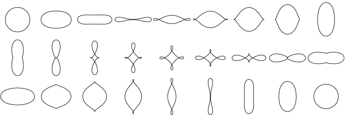
Figure 3. A great circle geodesic on $B_{\text{od}}$. The geodesic begins at the circle at the top left, runs from left to right, then to the second row and finally the third. It leaves $B_{\text{od}}$ twice: at the top right and bottom left, in both of which the singularity of figure 1 occurs in 2 places. The index of the curve changes from $+1$ to $-3$ in the middle row. See text.

5. Sectional curvature

We compute, in this section, the sectional curvature of $B_{i,{\text{od}}}/(\text{sim})$ (i.e., translations, rotations, scaling). We first compute the sectional curvature on the Grassmannian which is non-negative (but vanishes on many planes) and conclude from O’Neill’s formula [14] that the sectional curvature on $B_{i}/(\text{sim})$ is non-negative But since the O’Neill correction term is difficult to compute in this setting we also do it in a more explicit way, computing first the curvature on the Stiefel manifold by Gauss’ equation, then carrying it over to $\operatorname{Imm}/(\text{transl})$. Since this is an open subset in a Fréchet space, the O’Neill correction term can be computed more easily on $\operatorname{Imm}/(\text{transl})$ and so we finally get a more explicit formula for the sectional curvature on $B_{i}/(\text{transl})$.

5.1. Sectional curvature on $\operatorname{\bf Gr}(2,V)$

Let $W\in\operatorname{\bf Gr}(2,V)$ be a fixed 2-plane which we identify again with $\mathbb{R}^{2}$. Let $\eta:V\to V$ be the isomorphism which equals $-1$ on $W$ and $1$ on $W^{\bot}$ satisfying $\eta=\eta^{-1}$. Then the Grassmanian is the symmetric space $O(V)/(O(W)\times O(W^{\bot}))$ with the involutive automorphism $\sigma:O(V)\to O(V)$ given by $\sigma(U)=\eta.U\eta$. For the Lie algebra in the $V=W\oplus W^{\bot}$-decomposition we have

$$\begin{pmatrix}-1&0\\ 0&1\end{pmatrix}\begin{pmatrix}x&-y^{T}\\ y&U\end{pmatrix}\begin{pmatrix}-1&0\\ 0&1\end{pmatrix}=\begin{pmatrix}x&y^{T}\\ y&U\end{pmatrix}$$

Here $x\in L(W,W),y\in L(W,W^{\bot})$. The fixed point group is $O(V)^{\sigma}=O(W)\times O(W^{\bot})$. The reductive decomposition $\mathfrak{g}=\mathfrak{k}+\mathfrak{p}$ is given by

$$\left\{\begin{pmatrix}x&-y^{T}\\ y&U\end{pmatrix}\right\}=\left\{\begin{pmatrix}x&0\\ 0&U\end{pmatrix},x\in\mathfrak{s}\mathfrak{o}(2)\right\}+\left\{\begin{pmatrix}0&-y^{T}\\ y&0\end{pmatrix},y\in L(W,W^{\bot})\right\}$$

Let $\pi:O(V)\to O(V)/(O(W)\times O(W^{\bot}))=\operatorname{\bf Gr}(2,V)$ be the quotient projection. Then $T_{e}\pi:\mathfrak{p}\to T_{o}\operatorname{\bf Gr}$ is an isomorphism, and the $O(V)$-invariant Riemannian metric on $\operatorname{\bf Gr}(2,V)$ is given by

$$G^{\operatorname{\bf Gr}}_{o} (T_{e}\pi.Y_{1},T_{e}\pi.Y_{2})=-\tfrac{1}{2}\operatorname{tr}(Y_{1}Y_{2})=-\tfrac{1}{2}\operatorname{tr}\begin{pmatrix}0&-y_{1}^{T}\\ y_{1}&0\end{pmatrix}\begin{pmatrix}0&-y_{2}^{T}\\ y_{2}&0\end{pmatrix}$$

$$=-\tfrac{1}{2}\operatorname{tr}\begin{pmatrix}-y_{1}^{T}y_{2}&0\\ 0&-y_{1}y_{2}^{T}\end{pmatrix}=\tfrac{1}{2}\operatorname{tr}_{W}(y_{1}^{T}y_{2})+\tfrac{1}{2}\operatorname{tr}_{W^{\bot}}(y_{1}y_{2}^{T})$$

$$=\operatorname{tr}_{W}(y_{1}^{T}y_{2})=\langle y_{1}(e_{1}),y_{2}(e_{1})\rangle_{W^{\bot}}+\langle y_{1}(e_{2}),y_{2}(e_{2})\rangle_{W^{\bot}}$$

for $Y_{1},Y_{2}\in\mathfrak{p}$, where $e_{1},e_{2}$ is an orthonormal base of $W$. By the general theory of symmetric spaces [6], the curvature is given by

$$R^{\operatorname{\bf Gr}}_{o}(T_{e}\pi.Y_{1},T_{e}\pi.Y_{2})T_{e}\pi.Y_{1}=T_{e}\pi.[[Y_{1},Y_{2}],Y_{1}]$$

$$\left[\begin{pmatrix}0&-y_{1}^{T}\\ y_{1}&0\end{pmatrix},\begin{pmatrix}0&-y_{2}^{T}\\ y_{2}&0\end{pmatrix}\right]=\begin{pmatrix}-y_{1}^{T}y_{2}+y_{2}^{T}y_{1}\\ 0&-y_{1}y_{2}^{T}+y_{2}y_{1}^{T}\end{pmatrix}$$

$$\left[\left[\begin{pmatrix}0&-y_{1}^{T}\\ y_{1}&0\end{pmatrix},\begin{pmatrix}0&-y_{2}^{T}\\ y_{2}&0\end{pmatrix}\right],\begin{pmatrix}0&-y_{1}^{T}\\ y_{1}&0\end{pmatrix}\right]=$$

$$\qquad\qquad=\left[\begin{pmatrix}-y_{1}^{T}y_{2}+y_{2}^{T}y_{1}&0\\ 0&-y_{1}y_{2}^{T}+y_{2}y_{1}^{T}\end{pmatrix},\begin{pmatrix}0&-y_{1}^{T}\\ y_{1}&0\end{pmatrix}\right]$$

$$\qquad\qquad=\begin{pmatrix}0&2y_{1}^{T}y_{2}y_{1}^{T}-y_{2}^{T}y_{1}y_{1}^{T}-y_{1}^{T}y_{1}y_{2}^{T}\\ -2y_{1}y_{2}^{T}y_{1}+y_{2}y_{1}^{T}y_{1}+y_{1}y_{1}^{T}y_{2}&0\end{pmatrix}$$

For the sectional curvature we have (where we assume that $Y_{1},Y_{2}$ is orthonormal):

$$k^{\operatorname{\bf Gr}(2,V)}_{\operatorname{span}(Y_{1},Y_{2})} =-B(Y_{2},[[Y_{1},Y_{2}],Y_{1}])=\operatorname{tr}_{W}(y_{2}^{T}y_{2}y_{1}^{T}y_{1}+y_{2}^{T}y_{1}y_{1}^{T}y_{2}-2y_{2}^{T}y_{1}y_{2}^{T}y_{1})$$

$$=\tfrac{1}{2}\operatorname{tr}_{W}\big{(}(y_{2}^{T}y_{1}-y_{1}^{T}y_{2})^{T}(y_{2}^{T}y_{1}-y_{1}^{T}y_{2})\big{)}$$

$$\qquad+\tfrac{1}{2}\operatorname{tr}_{W^{\bot}}\big{(}(y_{2}y_{1}^{T}-y_{1}y_{2}^{T})^{T}(y_{2}y_{1}^{T}-y_{1}y_{2}^{T})\big{)}$$

$$=\tfrac{1}{2}\|y_{2}^{T}y_{1}-y_{1}^{T}y_{2}\|^{2}_{L^{2}(W,W)}+\tfrac{1}{2}\|y_{2}y_{1}^{T}-y_{1}y_{2}^{T}\|^{2}_{L^{2}(W^{\bot},W^{\bot})}\geq 0.$$

where $L^{2}$ stands for the space of Hilbert-Schmidt operators. Note that there are many orthonormal pairs $Y_{1},Y_{2}$ on which sectional curvature vanishes and that its maximum value 2 is attained when $y_{i}$ are isometries and $y_{2}=Jy_{1}$ where $J$ is rotation through angle $\pi/2$ in the image plane of $y_{1}$.

5.2. Sectional curvature on $\operatorname{Imm/(sim)}$

The curvature formula can be rewritten by ‘lowering the indices’ which will make it much easier to express it in terms of the immersion $c$. Fix an orthonormal basis $e,f$ of $W$ and let $\delta e_{k}=y_{k}(e),\delta f_{k}=y_{k}(f)$. For $x,y\in W^{\bot}$, we use the notation $x\wedge y=x\otimes y-y\otimes x\in W^{\bot}\otimes W^{\bot}.$ Then:

$$k^{\operatorname{\bf Gr}(2,V)}_{\operatorname{span}(Y_{1},Y_{2})}=(\langle\delta e_{1},\delta f_{2}\rangle-\langle\delta e_{2},\delta f_{1}\rangle)^{2}+\tfrac{1}{2}\|\delta e_{1}\wedge\delta e_{2}+\delta f_{1}\wedge\delta f_{2}\|^{2}.$$

To check this, note that $y_{2}^{T}y_{1}-y_{1}^{T}y_{2}$ is given by a skew-symmetric $2\times 2$ matrix whose off diagonal entry is just $\langle\delta e_{1},\delta f_{2}\rangle-\langle\delta e_{2},\delta f_{1}\rangle$ and this identifies the first terms in the two formulas for $k$. On the other hand, $y_{2}y_{1}^{T}$ is given by a matrix of rank 2 on the infinite dimensional space $W^{\bot}$. In view of $W^{\bot}\otimes W^{\bot}\subset L(W^{\bot},W^{\bot})$ it is the 2-tensor $\delta e_{1}\otimes\delta e_{2}+\delta f_{1}\otimes\delta f_{2}$. Skew-symmetrizing, we identify the second terms in the two expressions for $k$.

Going over to the immersion $c$, the tangent vector $\delta e_{k}+i\delta f_{k}$ to $\operatorname{\bf Gr}$ becomes the tangent vector $h_{k}=\delta c=\int(\delta e_{k}+i\delta f_{k})(e+if)d\theta$ to $\operatorname{Imm/(sim)}$. To express the first term in the curvature, we have:

Proposition.

$\langle\delta e_{1},\delta f_{2}\rangle-\langle\delta e_{2},\delta f_{1}\rangle=\int_{C}\det(D_{s}h_{1},D_{s}h_{2})ds.$

Proof.

$$D_{s}(h_{k})=\frac{(e+if).(\delta e_{k}+i\delta f_{k})}{e^{2}+f^{2}}$$

hence

$$\det(D_{s}h_{1},D_{s}h_{2})=\mathrm{Im}(\overline{D_{s}h_{1}},D_{s}h_{2})=\frac{\mathrm{Im}\left((\delta e_{1}-i\delta f_{1})(\delta e_{2}+i\delta f_{2})\right)}{e^{2}+f^{2}}$$

hence

$$\int_{C}\det(D_{s}h_{1},D_{s}h_{2})ds=\int_{S^{1}}(\delta e_{1}\delta f_{2}-\delta e_{2}\delta f_{1})d\theta.$$

∎

The second term is not quite so compact: because it is a norm on $W^{\bot}\otimes W^{\bot}$, it requires double integrals over $C\times C$, not just a simple integral over $C$. We use the notation as above $c(\theta)=r(\theta)e^{i\alpha(\theta)}$. Then we have:

Proposition.

$$\|\delta e_{1}\wedge\delta e_{2}+\delta f_{1}\wedge\delta f_{2}\|^{2}=\mathrm{term1}+\mathrm{term2}$$

$$\mathrm{term1}=\iint\limits_{C\times C}\frac{1+\cos(\alpha(x)-\alpha(y))}{2}\cdot\left(\begin{array}[]{l}\langle D_{s}h_{1}(x),D_{s}h_{2}(y)\rangle\\ -\langle D_{s}h_{2}(x),D_{s}h_{1}(y)\rangle\end{array}\right)^{2}ds(x)ds(y)$$

$$\mathrm{term2}=\iint\limits_{C\times C}\frac{1-\cos(\alpha(x)-\alpha(y))}{2}\cdot\left(\begin{array}[]{l}\det(D_{s}h_{1}(x),D_{s}h_{2}(y))\\ -\det(D_{s}h_{2}(x),D_{s}h_{1}(y))\end{array}\right)^{2}ds(x)ds(y)$$

Proof. Using $r$ and $\alpha$, we have: $\sqrt{r}e^{-i\alpha/2}D_{s}h_{k}=\delta e_{k}+i\delta f_{k},$ hence:

$$\sqrt{r(x)r(y)}e^{\frac{i(\alpha(x)-\alpha(y)}{2}}\overline{D_{s}h_{1}(x)}D_{s}h_{2}(y)=\delta e_{1}(x)\delta e_{2}(y)+\delta f_{1}(x)\delta f_{2}(y)+i(\cdots)$$

Skew-symmetrizing in the 2 vectors $h_{1},h_{2}$, we get:

$$\sqrt{r(x)r(y)}\mathrm{Re}\left\{e^{\frac{i(\alpha(x)-\alpha(y))}{2}}\left(\overline{D_{s}h_{1}(x)}D_{s}h_{2}(y)-\overline{D_{s}h_{2}(x)}D_{s}h_{1}(y)\right)\right\}=\\ \delta e_{1}(x)\delta e_{2}(y)-\delta e_{2}(x)\delta e_{1}(y)+\delta f_{1}(x)\delta f_{2}(y)-\delta f_{2}(x)\delta f_{1}(y).$$

Squaring and integrating over $S^{1}\times S^{1}$, the right hand becomes $\|\delta e_{1}\wedge\delta e_{2}+\delta f_{1}\wedge\delta f_{2}\|^{2}$. On the left, first write $\mathrm{Re}(e^{i(\alpha(x)-\alpha(y))/2}(\cdots))$ as the sum of $\cos((\alpha(x)-\alpha(y))/2)\mathrm{Re}(\cdots)$ and $-\sin((\alpha(x)-\alpha(y))/2)\mathrm{Im}(\cdots)$. Then when we square and integrate, the cross term drops out because it is odd when $x,y$ are reversed. ∎

We therefore obtain the expression of the curvature in $\operatorname{Imm/(sim)}$:

$$k^{\operatorname{Imm}/(\text{sim})}_{\mathrm{span}(h_{1},h_{2})}=\Big{(}\int_{C}\det(D_{s}h_{1},D_{s}h_{2})ds\Big{)}^{2}+$$

(11) $$\quad+\iint\limits_{C\times C}\frac{1+\cos(\alpha(x)-\alpha(y))}{2}\cdot\left(\begin{array}[]{l}\langle D_{s}h_{1}(x),D_{s}h_{2}(y)\rangle\\ -\langle D_{s}h_{2}(x),D_{s}h_{1}(y)\rangle\end{array}\right)^{2}ds(x)ds(y)+$$

(14) $$\quad+\iint\limits_{C\times C}\frac{1-\cos(\alpha(x)-\alpha(y))}{2}\cdot\left(\begin{array}[]{l}\det(D_{s}h_{1}(x),D_{s}h_{2}(y))\\ -\det(D_{s}h_{2}(x),D_{s}h_{1}(y))\end{array}\right)^{2}ds(x)ds(y)$$

A major consequence of the calculation for the curvature on the Grassmannian is:

5.3 Theorem.

The sectional curvature on $B_{i}/(\operatorname{sim})$ is $\geq 0$.

Proof. We apply O’Neill’s formula [14] to the Riemannian submersion

$$\pi:\operatorname{\bf Gr}^{0}\to\operatorname{\bf Gr}^{0}/U(V)\cong B_{i}/\operatorname{Diff}^{+}(S^{1})$$

$$k^{\operatorname{\bf Gr}^{0}\!\!/U(V)}_{\pi(W)}(X,Y)=k^{\operatorname{\bf Gr}^{0}}_{W}(X^{\text{hor}},Y^{\text{hor}})+\tfrac{3}{4}\|[X^{\text{hor}},Y^{\text{hor}}]^{\text{ver}}|_{W}\|^{2}\geq 0$$

where $X^{\text{hor}}$ is a horizontal vector field projecting to a vector field $X$ at $\pi(W)$; similarly for $Y$. The horizontal and vertical projections exist and are pseudo differential operators, see 5.6. ∎

5.4. Sectional curvature on $\operatorname{\bf St}(2,V)$

The Stiefel manifold is not a symmetric space (as the Grassmannian); it is a homogeneous Riemannian manifold. This can be used to compute its sectional curvature. But the following procedure is simpler:

For $(e,f)\in V^{2}$ we consider the functions

$$Q_{1}(e,f)=\frac{1}{2}\|e\|^{2},\quad Q_{2}(e,f)=\frac{1}{2}\|f\|^{2}\text{ and }Q_{3}(e,f)=\frac{1}{\sqrt{2}}{\left\langle{e}\,,\,{f}\right\rangle}.$$

Then $\operatorname{\bf St}(2,V)$ is the codimension 3 submanifold of $V^{2}$ defined by the equations $Q_{1}=Q_{2}=1/2$, $Q_{3}=0$.

The metric on $\operatorname{\bf St}(2,V)$ is induced by the metric on $V^{2}$. If ${\xi_{1}}=(\delta e_{1},\delta f_{1})$ and ${\xi_{2}}=(\delta e_{2},\delta f_{2})$ are tangent vectors at a point in $V^{2}$, we have ${\left\langle{{\xi_{1}}}\,,\,{{\xi_{2}}}\right\rangle}={\left\langle{\delta e_{1}}\,,\,{\delta e_{2}}\right\rangle}+{\left\langle{\delta f_{1}}\,,\,{\delta f_{2}}\right\rangle}$. For a function $\varphi$ on $V^{2}$ its gradient $\operatorname{grad}\varphi$ of $\varphi$ (if it exists) is given by $\langle\operatorname{grad}\varphi(v),\xi\rangle=d\varphi(v)(\xi)=D_{v,\xi}\varphi$. The following are the gradients of $Q_{i}$:

$$\operatorname{grad}Q_{1}=(e,0),\quad\operatorname{grad}Q_{2}=(0,f),\quad\operatorname{grad}Q_{3}=\frac{1}{\sqrt{2}}(f,e),$$

and these form an orthonormal basis of the normal bundle $\operatorname{Nor}(\operatorname{\bf St})$ of $\operatorname{\bf St}(2,V)$. Let ${\xi_{1}},{\xi_{2}}$ be two normal unit vectors tangent to $\operatorname{\bf St}(2,V)$ at a point $(e,f)$. Since $V^{2}$ is flat the sectional curvature of $\operatorname{\bf St}(2,V)$ is given by the Gauss formula [4]:

$$k^{\operatorname{\bf St}(2,V)}_{\mathrm{span}(\xi_{1},\xi_{2})}=\langle S({\xi_{1}},{\xi_{1}}),S({\xi_{2}},{\xi_{2}})\rangle-\langle S({\xi_{1}},{\xi_{2}}),S({\xi_{1}},{\xi_{2}})\rangle$$

where $S$ denotes the second fundamental form of $\operatorname{\bf St}(2,V)$ in $V^{2}$. Moreover, when a manifold is given as the zeros of functions $F_{k}$ in a flat ambient space whose gradients are orthonormal, the second fundamental form is given by:

$$S(X,Y)=\sum_{k}H_{F_{k}}(X,Y)\cdot\mathrm{grad}F_{k}$$

where $H$ is the Hessian of second derivatives. Given $\xi_{1},\xi_{2}\in T_{(e,f)}\operatorname{\bf St}$ with $\xi_{i}=(\delta e_{i},\delta f_{i})$, we have:

$$H_{Q_{1}}(\xi_{1},\xi_{2})=\langle\delta e_{1},\delta e_{2}\rangle,\quad H_{Q_{2}}(\xi_{1},\xi_{2})=\langle\delta f_{1},\delta f_{2}\rangle,$$

$$H_{Q_{3}}(\xi_{1},\xi_{2})=\tfrac{1}{\sqrt{2}}\big{(}\langle\delta e_{1},\delta f_{2}\rangle+\langle\delta e_{2},\delta f_{1}\rangle\big{)}$$

so that

$$S(\mathbf{\xi}_{1},\mathbf{\xi}_{2})=-\langle\delta e_{1},\delta e_{2}\rangle\operatorname{grad}Q_{1}-\langle\delta f_{1},\delta f_{2}\rangle\operatorname{grad}Q_{2}\\ -\tfrac{1}{\sqrt{2}}\big{(}\langle\delta f_{1},\delta e_{2}\rangle+\langle\delta e_{1},\delta f_{2}\rangle\big{)}\operatorname{grad}Q_{3}.$$

Finally, the sectional curvature of $\operatorname{\bf St}(2,V)$ for a normal pair of unit vectors $\mathbf{\xi},\mathbf{\eta}$ in $T_{\mathbf{f}}\operatorname{\bf St}(2,V)$ is given by:

$$k^{\operatorname{\bf St}(2,V)}_{\mathrm{span}(\xi_{1},\xi_{2})} =\|\delta e_{1}\|^{2}\|\delta e_{2}\|^{2}+\|\delta f_{1}\|^{2}\|\delta f_{2}\|^{2}+2\langle\delta e_{1},\delta f_{1}\rangle\langle\delta e_{2},\delta f_{2}\rangle$$

$$\quad-\langle\delta e_{1},\delta e_{2}\rangle^{2}-\langle\delta f_{1},\delta f_{2}\rangle^{2}-\tfrac{1}{2}(\langle\delta e_{1},\delta f_{2}\rangle+\langle\delta f_{1},\delta e_{2}\rangle)^{2}$$

(15) $$=\tfrac{1}{2}\|\delta e_{1}\otimes\delta e_{2}-\delta e_{2}\otimes\delta e_{1}+\delta f_{1}\otimes\delta f_{2}-\delta f_{2}\otimes\delta f_{1}\|^{2}$$

$$\quad-\tfrac{1}{2}(\langle\delta e_{1},\delta f_{2}\rangle-\langle\delta e_{2},\delta f_{1}\rangle)^{2}$$

Comparing this with the curvature for the Grasmannian, we see that the O’Neill factor in this case is $\tfrac{3}{2}(\langle\delta e_{1},\delta f_{2}\rangle+\langle\delta f_{1},\delta e_{2}\rangle)^{2}$. Moreover, we can write for the curvature of the isometric $\operatorname{Imm/(transl,scal)}$

$$k^{\operatorname{Imm/(transl,scal)}}_{\mathrm{span}(h_{1},h_{2})}=-\tfrac{1}{2}\left(\int_{C}\det(D_{s}h_{1},D_{s}h_{2})ds\right)^{2}+$$

(18) $$+\tfrac{1}{2}\iint\limits_{C\times C}\frac{1+\cos(\alpha(x)-\alpha(y))}{2}\cdot\left(\begin{array}[]{l}\langle D_{s}h_{1}(x),D_{s}h_{2}(y)\rangle-\\ -\langle D_{s}h_{2}(x),D_{s}h_{1}(y)\rangle\end{array}\right)^{2}ds(x)ds(y)+$$

(21) $$+\tfrac{1}{2}\iint\limits_{C\times C}\frac{1-\cos(\alpha(x)-\alpha(y))}{2}\cdot\left(\begin{array}[]{l}\det(D_{s}h_{1}(x),D_{s}h_{2}(y))-\\ -\det(D_{s}h_{2}(x),D_{s}h_{1}(y))\end{array}\right)^{2}ds(x)ds(y)$$

5.5. Sectional curvature on the unscaled Stiefel manifold

Using the basic mapping $\Phi$, the manifold $\operatorname{Imm}/(\text{transl})$ can be identified with the unscaled Stiefel manifold which we view as the following submanifold of $V^{2}$. We do not introduce a systematic notation for it.

(22) $$M=\{(e,f)\in V^{2}\setminus\{(0,0)\},\|e\|^{2}=\|f\|^{2}\text{ and }{\left\langle{e}\,,\,{f}\right\rangle}=0\}$$

equipped with the metric

$$\|(\delta e,\delta f)\|_{(e,f)}^{2}=2\frac{\|\delta e\|^{2}+\|\delta f\|^{2}}{\|e\|^{2}+\|f\|^{2}}.$$

Consider the diffeomorphism $\Psi:\mathbb{R}^{+}\times\operatorname{\bf St}(2,V)\to M$ defined by

$$\Psi(\ell,(e,f))=(\sqrt{\ell}.e,\sqrt{\ell}.f)=:(\bar{e},\bar{f}).$$

For $\xi(\delta e,\delta f)\in T_{(e,f)}\operatorname{\bf St}$ we have

$$T_{(\ell,e,f)}\Psi.(\lambda,\xi)=\Big{(}\frac{\lambda}{2\sqrt{\ell}}e+\sqrt{\ell}.\delta e,\frac{\lambda}{2\sqrt{\ell}}f+\sqrt{\ell}.\delta f\Big{)}=:(\bar{\delta}e,\bar{\delta}f)$$

Thus, $\Psi$ is an isometry if $\mathbb{R}^{+}\times\operatorname{\bf St}(2,V)$ is equipped with the metric

$$\|(\lambda,\xi)\|^{2}_{\ell,(e,f)}=\frac{\lambda^{2}}{2\ell^{2}}+\|\delta e\|^{2}+\|\delta f\|^{2}$$

so that $M$ is isometric to the Riemannian product of $\mathbb{R}^{+}$ and $\operatorname{\bf St}(2,V)$, taking $\|\lambda\|_{\ell}=|\lambda|/(\sqrt{2}.\ell)$ for the metric on $\mathbb{R}^{+}$. This implies that the curvature tensor on $M$ is the sum of the tensors on $\mathbb{R}^{+}$ (which vanishes) and $\operatorname{\bf St}(2,V)$. Thus, if $\bar{\xi}_{i}=T_{(\ell,f)}\pi.(\lambda,\xi_{i})$, $i=1,2$ with $(\xi_{1},\xi_{1})$ orthonormal,

$$k^{M}_{\mathrm{span}(\bar{\xi}_{1},\bar{\xi}_{2})} =\frac{-\langle R_{M}(\bar{\xi}_{1},\bar{\xi}_{2})\bar{\xi}_{1},\bar{\xi}_{2}\rangle}{\|\bar{\xi}_{1}\|^{2}\|\bar{\xi}_{2}\|^{2}-\langle\bar{\xi}_{1},\bar{\xi}_{2}\rangle^{2}}=\frac{-\langle R_{\operatorname{\bf St}}(\xi_{1},\xi_{2})\xi_{1},\xi_{2}\rangle}{\|\bar{\xi}_{1}\|^{2}\|\bar{\xi}_{2}\|^{2}-\langle\bar{\xi}_{1},\bar{\xi}_{2}\rangle^{2}}$$

$$=\frac{k^{\operatorname{\bf St}}_{\mathrm{span}(\xi_{1},\xi_{2})}}{\|\bar{\xi}_{1}\|^{2}\|\bar{\xi}_{2}\|^{2}-\langle\bar{\xi}_{1},\bar{\xi}_{2}\rangle^{2}}$$

Note that we have the relations:

(23) $$\delta\bar{e} = \frac{\lambda}{2\sqrt{\ell}}e+\sqrt{\ell}.\delta e$$

$$\delta\bar{f} = \frac{\lambda}{2\sqrt{\ell}}f+\sqrt{\ell}.\delta f$$

5.6. O’Neill’s formula

For Riemannian submersions, O’Neill formula [14] states that the sectional curvature, in the plane generated by two horizontal vectors, is given by the curvature computed on the space “above” plus a positive correction term given by $(3/4)$ times the squared norm of the vertical projection of the Lie bracket of any horizontal extensions of the two vectors. We now proceed to the computation of this correction for the submersion from $\operatorname{Imm}/\mathrm{(sim)}$ to $B_{i}/\mathrm{(sim)}$.

Because of the simplicity of local charts there, it will be easier to start from $\operatorname{Imm}/\mathrm{(transl)}$. Let $c\in\operatorname{Imm}$ with $\int_{S^{1}}c\,ds=0$. We first compute the vertical projection of a vector $h\in T_{c}\operatorname{Imm}/(\text{transl})$ for the submersion $\operatorname{Imm}/\mathrm{(transl)}\to B_{i}/\mathrm{(sim)}$. Vectors in the vertical space at $c$ take the form

$$\tilde{h}=bv+i\alpha c+\beta c,$$

each generator corresponding (in this order) to the action of diffeomorphisms, rotation and scaling ($b$ is a function and $\alpha,\beta$ are constants). Denoting $h^{\top}$ the vertical projection of $h$, and using the fact that $G_{c}(h,\tilde{h})=G_{c}(h^{\top},\tilde{h})$ for any vertical $\tilde{h}$, we easily obtain the fact that

$$h^{\top}=bv+i\alpha c+\beta c,$$

with

$$L^{\top}b+\alpha\kappa = v\cdot Lh,$$

$$\overline{\left\langle{b\kappa}\right\rangle}+\alpha = \overline{\left\langle{D_{s}h\cdot n}\right\rangle},$$

$$\beta = \overline{\left\langle{D_{s}h\cdot v}\right\rangle},$$

where we have used the following notation: $Lh=-D_{s}^{2}h$, $L^{\top}b=-D_{s}^{2}b+\kappa^{2}b$ and, as before

$$\overline{\left\langle{F}\right\rangle}=\frac{1}{\ell}\int Fds.$$

From this, we obtain the fact that $b$ must satisfy

(25) $$L^{\top}b-\overline{\left\langle{b\kappa}\right\rangle}\kappa=v\cdot Lh-\overline{\left\langle{D_{s}h\cdot n}\right\rangle}\kappa.$$

The operator $L^{\top}$ is of order two, unbounded, selfadjoint, and positive on $\{f\in L^{2}(S^{1},ds):\int fds=0\}$ thus it is invertible on $\{f\in C^{\infty}(S^{1},\mathbb{R}):\int f\,ds=0\}$ by an index argument as given in lemma [11, 4.5]. The operator $\tilde{L}^{\top}$ in the left-hand side of (25) is also invertible under the condition that $c$ is not a circle, with an inverse given by

(26) $$(\tilde{L}^{\top})^{-1}\psi=(L^{\top})^{-1}\psi+\frac{\overline{\left\langle{(L^{\top})^{-1}\psi\kappa}\right\rangle}}{1-\overline{\left\langle{\kappa(L^{\top})^{-1}\kappa}\right\rangle}}(L^{\top})^{-1}\kappa.$$

This is well defined unless $\kappa\equiv\mathrm{constant}$. Indeed, letting $f=(L^{\top})^{-1}\kappa$, we have $-fD_{s}^{2}f+\kappa^{2}f^{2}=\kappa f$ which implies $\overline{\left\langle{\kappa f}\right\rangle}\geq\overline{\left\langle{\kappa^{2}f^{2}}\right\rangle}$. By Schwartz inequality we have $\overline{\left\langle{\kappa f}\right\rangle}\leq(\overline{\left\langle{\kappa^{2}f^{2}}\right\rangle})^{1/2}$ which ensures $\overline{\left\langle{\kappa f}\right\rangle}\leq 1.$ Equality requires $\overline{\left\langle{fD_{s}^{2}f}\right\rangle}=0$ or $f=\text{constant}$, which in turn implies that $\kappa=\text{constant}$ and that $c$ is a circle. We note for future use that $(\tilde{L}^{\top})^{-1}\kappa=(L^{\top})^{-1}\kappa$.

We hereafter assume that $c$ has length 1, is parametrized with its arc-length divided by $2\pi$, and that it is different from the unit circle (which is a singular point in $B_{i}/(\mathrm{sim})$). We can therefore write

(27) $$h^{\top}=\left((\tilde{L}^{\top})^{-1}\psi(h)v-i\overline{\left\langle{\kappa(\tilde{L}^{\top})^{-1}\psi(h)}\right\rangle}c\right)+i\overline{\left\langle{D_{s}h\cdot v}\right\rangle}c+\overline{\left\langle{D_{s}h\cdot n}\right\rangle}c$$

with $\psi(h)=v\cdot Lh-\overline{\left\langle{D_{s}h\cdot n}\right\rangle}\kappa$.

The right-hand term in (27) is the sum of three orthogonal terms, the last two forming the vertical projection for the submersion $\operatorname{Imm}/(\mathrm{transl})\to\operatorname{Imm}/(\mathrm{sim})$. Applying O’Neill’s formula two times to this submersion and to $\operatorname{Imm}/(\mathrm{sim})\to B_{i}/(\mathrm{sim})$, we see that the correcting term for the sectional curvature on $B_{i}/(\mathrm{sim})$ relative to the curvature on $\operatorname{Imm}/(\mathrm{sim})$, in the direction of the horizontal vectors $h_{1}$ and $h_{2}$ is

$$\rho(h_{1},h_{2})_{c}=\frac{3}{4}\left\|(\tilde{L}^{\top})^{-1}\psi([\bar{h}_{1},\bar{h}_{2}]_{c})v-i\overline{\left\langle{\kappa(\tilde{L}^{\top})^{-1}\psi([\bar{h}_{1},\bar{h}_{2}]_{c})}\right\rangle}c\right\|^{2},$$

$\bar{h}_{1},\bar{h}_{2}$ being horizontal extensions of $h_{1}$ and $h_{2}$. From the identity

$$\|bv-i\overline{\left\langle{\kappa b}\right\rangle}c\|_{c}^{2} = \int|b^{\prime}v+\kappa bn-\overline{\left\langle{\kappa b}\right\rangle}n|^{2}ds$$

$$= \int(bLb+\kappa^{2}b^{2}n-\overline{\left\langle{\kappa b}\right\rangle}\kappa b)ds$$

$$= \int b(\tilde{L}^{T}b)ds$$

we can write

$$\rho(h_{1},h_{2})_{c}=\frac{3}{4}\int\psi([\bar{h}_{1},\bar{h}_{2}]_{c})(\tilde{L}^{\top})^{-1}\psi([\bar{h}_{1},\bar{h}_{2}]_{c})ds.$$

We now proceed to the computation of the Lie bracket:

5.7 Proposition.

$\psi([h_{1}^{\bot},h_{2}^{\bot}]_{c})=W_{s}(D_{s}h_{1}\cdot n,D_{s}h_{2}\cdot n)-\overline{\left\langle{\mathrm{det}(D_{s}h_{1},D_{s}h_{2})}\right\rangle}\kappa$ where $W_{s}(h,k)=hD_{s}k-kD_{s}h$ is the Wronskian with respect to the arc-length parameter.

Proof. We take $h_{1},h_{2}\in\{f\in C^{\infty}(S^{1},\mathbb{R}^{2}):\int f\,ds=0\}$ which are horizontal at $c$, consider them as constant vector fields on $\operatorname{Imm}/(\text{transl})$ and take, as horizontal extensions, their horizontal projections $\gamma\mapsto h_{1}^{\bot}(\gamma),h_{2}^{\bot}(\gamma)$. Then we compute the Lie bracket evaluated at $\gamma$:

$$[h_{1}^{\bot},h_{2}^{\bot}]\Big{|}_{\gamma} = D_{c,h_{2}}h_{1}^{\bot}(\gamma)-D_{c,h_{1}}h_{2}^{\bot}(\gamma)$$

$$= -D_{c,h_{2}}h_{1}^{\top}(\gamma)+D_{c,h_{1}}h_{2}^{\top}(\gamma)$$

since $h_{i}^{\top}+h_{i}^{\bot}=h_{i}$ is constant, for $i=1,2$. We have

$$h_{1}^{\top}(\gamma) = \left((\tilde{L}^{\top}_{\gamma})^{-1}\psi_{\gamma}(h_{1})v_{\gamma}-i\overline{\left\langle{\kappa_{\gamma}(\tilde{L}^{\top}_{\gamma})^{-1}\psi_{\gamma}}\right\rangle}_{\gamma}\gamma\right)$$

$$+ i\overline{\left\langle{D_{s_{\gamma}}h_{1}\cdot n_{\gamma}}\right\rangle}_{\gamma}\gamma+\overline{\left\langle{D_{s_{\gamma}}h_{1}\cdot v_{\gamma}}\right\rangle}_{\gamma}\gamma$$

with $\psi_{\gamma}(h_{1})=v_{\gamma}\cdot L_{\gamma}h_{1}-\overline{\left\langle{D_{s_{\gamma}}h_{1}\cdot v_{\gamma}}\right\rangle}_{\gamma}\kappa_{\gamma}$. We have added subscripts $\gamma$ to quantities that depend on the curve, with $D_{s_{\gamma}}$ holding for the derivative with respect to the $\gamma$ arc-length (we still use no subscript for $\gamma=c$). Note that $\overline{\left\langle{D_{s_{\gamma}}h_{1}\cdot n_{\gamma}}\right\rangle}_{\gamma}=\ell_{\gamma}\overline{\left\langle{D_{s}h_{1}\cdot n_{\gamma}}\right\rangle}$ and $\overline{\left\langle{D_{s_{\gamma}}h_{1}\cdot v_{\gamma}}\right\rangle}_{\gamma}=\ell_{\gamma}\overline{\left\langle{D_{s}h_{1}\cdot v_{\gamma}}\right\rangle}$ which is a first simplification. Also, since we assume that $h_{1}$ is horizontal at $c$, we have $\overline{\left\langle{D_{s}h_{1}\cdot n}\right\rangle}=\overline{\left\langle{D_{s}h_{1}\cdot v}\right\rangle}=0$ and $v\cdot Lh_{1}=0$, which imply $\psi(h_{1})=0$.

We therefore have (to simplify, we temporarily use the notation $f^{\prime}=D_{s}f$)

$$D_{c,h_{2}}h_{1}^{\top} = \left((\tilde{L}^{\top})^{-1}D_{c,h_{2}}\psi_{\gamma}(h_{1})v-i\overline{\left\langle{\kappa(\tilde{L}^{\top})^{-1}D_{c,h_{2}}\psi_{\gamma}(h_{1})}\right\rangle}c\right)$$

$$+ i\overline{\left\langle{h^{\prime}_{1}\cdot D_{c,h_{2}}n_{\gamma}}\right\rangle}c+\overline{\left\langle{h^{\prime}_{1}\cdot D_{c,h_{2}}v_{\gamma}}\right\rangle}c.$$

Since we have $D_{c,h_{2}}v_{\gamma}=(h^{\prime}_{2}\cdot n)n$ and $D_{c,h_{2}}n_{\gamma}=-(h^{\prime}_{2}\cdot n)v$ we immediately obtain the expression of the last two terms in (5.6), which are

(29) $$-i\overline{\left\langle{(h^{\prime}_{1}\cdot v)(h^{\prime}_{2}\cdot n)}\right\rangle}c+\overline{\left\langle{(h^{\prime}_{1}\cdot n)(h^{\prime}_{2}\cdot n)}\right\rangle}c.$$

We now focus on the variation of $\phi_{\gamma}$. We need to compute

$$D_{c,h_{2}}\psi_{\gamma}(h_{1}) = D_{c,h_{2}}(v_{\gamma}\cdot L_{\gamma}h_{1})-\overline{\left\langle{(h^{\prime}_{1}\cdot v)(h^{\prime}_{2}\cdot n)}\right\rangle}\kappa.$$

If $h$ is a constant vector field, we have

$$D_{s_{\gamma}}h=h^{\prime}\|\gamma^{\prime}\|^{-1}$$

and

$$L_{\gamma}h=-(h^{\prime}\|\gamma^{\prime}\|^{-1})^{\prime}\|\gamma^{\prime}\|^{-1}.$$

This implies

$$D_{c,h_{2}}L_{\gamma}h_{1} =-h^{\prime\prime}_{1}D_{c,h_{2}}\|\gamma^{\prime}\|^{-1}-(h^{\prime}_{1}D_{c,h_{2}}\|D_{s}\gamma\|^{-1})^{\prime}$$

$$=2h^{\prime\prime}_{1}(h^{\prime}_{2}\cdot v)+h^{\prime}_{1}(h^{\prime}_{2}\cdot v)^{\prime}.$$

Therefore

$$D_{c,h_{2}}(L_{\gamma}h_{1}\cdot v_{\gamma}) =(h^{\prime}_{1}\cdot v)(h^{\prime}_{2}\cdot v)^{\prime}-(h^{\prime\prime}_{1}\cdot n)(h^{\prime}_{2}\cdot n).$$

Using

$$h^{\prime\prime}_{1} =((h^{\prime}_{1}\cdot v)v+(h^{\prime}_{1}\cdot n)n)^{\prime}$$

$$=((h^{\prime}_{1}\cdot v)^{\prime}-\kappa(h^{\prime}_{1}\cdot n))v+((h^{\prime}_{1}\cdot n)^{\prime}+\kappa(h^{\prime}_{1}\cdot v))n$$

and the fact that $h^{\prime\prime}_{1}\cdot v=h^{\prime\prime}_{2}\cdot v=0$, we can write

$$D_{c,h_{2}}(L_{\gamma}h_{1}\cdot v_{\gamma}) =-(h^{\prime}_{2}\cdot n)(h^{\prime}_{1}\cdot n)^{\prime}$$

which yields

$$D_{c,h_{2}}\psi_{\gamma}(h_{1})=-(h^{\prime}_{2}\cdot n)(h^{\prime}_{1}\cdot n)^{\prime}-\overline{\left\langle{(h^{\prime}_{1}\cdot v)(h^{\prime}_{2}\cdot n)}\right\rangle}\kappa.$$

By symmetry

$$D_{c,h_{2}}\psi_{\gamma}(h_{1})-D_{c,h_{1}}\psi_{\gamma}(h_{2})=W_{s}(h^{\prime}_{1}\cdot n,h^{\prime}_{2}\cdot n)-\overline{\left\langle{\text{det}(h^{\prime}_{1},h^{\prime}_{2})}\right\rangle}\kappa,$$

where $W_{s}(\varphi_{1},\varphi_{2})=\varphi_{1}\varphi_{2}^{\prime}-\varphi_{1}^{\prime}\varphi_{2}.$

Combining this with (29), we get

$$[h^{\bot}_{1},h_{2}^{\bot}]_{c} = (\tilde{L}^{\top})^{-1}(W_{s}(h^{\prime}_{1}\cdot n,h^{\prime}_{2}\cdot n)-\overline{\left\langle{\mathrm{det}(h^{\prime}_{1},h^{\prime}_{2})}\right\rangle}\kappa)v$$

$$- i\overline{\left\langle{\kappa(\tilde{L}^{\top})^{-1}(W_{s}(h^{\prime}_{1}\cdot n,h^{\prime}_{2}\cdot n)-\overline{\left\langle{\mathrm{det}(h^{\prime}_{1},h^{\prime}_{2})}\right\rangle}\kappa)}\right\rangle}c-i\overline{\left\langle{\mathrm{det}(h^{\prime}_{1},h^{\prime}_{2})}\right\rangle}c$$

so that

$$\psi([h_{1}^{\bot},h_{2}^{\bot}]_{c}) = W_{s}(h^{\prime}_{1}\cdot n,k^{\prime}_{2}\cdot n)-\overline{\left\langle{\mathrm{det}(h^{\prime}_{1},h^{\prime}_{2})}\right\rangle}\kappa.$$

(We have used the fact that $\psi(bv+i\alpha c)=\tilde{L}^{\top}b$.) ∎

We therefore obtain the formula

(30) $$\rho(h_{1},h_{2})_{c}=\frac{3}{4}\int\Big{(}W_{s}(D_{s}h_{1}\cdot n,D_{s}h_{2}\cdot n)-\overline{\left\langle{\mathrm{det}(D_{s}h_{1},D_{s}h_{2})}\right\rangle}\kappa\Big{)}\cdot\\ \cdot(\tilde{L}^{\top})^{-1}\Big{(}W_{s}(D_{s}h_{1}\cdot n,D_{s}h_{2}\cdot n)-\overline{\left\langle{\mathrm{det}(D_{s}h_{1},D_{s}h_{2})}\right\rangle}\kappa\Big{)}ds$$

with $(\tilde{L}^{\top})^{-1}$ given by (26). Finally, assuming that $h_{1}$ and $h_{2}$ are orthogonal,

$$k_{\mathrm{span}(h_{1},h_{2})}^{\operatorname{B_{i}/(\text{sim})}} =k_{\mathrm{span}(h_{1},h_{2})}^{\operatorname{Imm/(\text{sim})}}+\rho(h_{1},h_{2})_{c}$$

where $k_{\mathrm{span}(h_{1},h_{2})}^{\operatorname{Imm/(\text{sim})}}$ is given in (11).

A similar (and simpler) computation provides the correcting term for the space $B_{i}/(\mathrm{transl,scale})$. In this case, the rotation part of the vertical space disappears, and the two remaining components (parametrization and scale) are orthogonal. The result is

(31) $$\rho(h_{1},h_{2})_{c}=\frac{3}{4}\int W_{s}(D_{s}h_{1}\cdot n,D_{s}h_{2}\cdot n)(L^{\top})^{-1}W_{s}(D_{s}h_{1}\cdot n,D_{s}h_{2}\cdot n)ds.$$

5.8. An upper bound for $k^{\operatorname{B_{i}/(\text{sim})}}_{\mathrm{span}(h_{1},h_{2})}$

Here we derive an explicit upper bound for $k^{B_{i}/(\text{sim})}_{\mathrm{span}(h_{1},h_{2})}$ at a fixed curve $c\in\operatorname{B_{i}/(sim)}$ and a fixed tangent vector $h_{2}$. This will show that geodesics (such as the one in the $h_{1}$ direction) have at least a small interval before they meet another geodesic. The size of this interval can be controlled, as we will see, by an upper bound that involves the supremum norm of the first two derivatives of $h_{1}$.

We assume that $c$ has length $2\pi$. Since $\operatorname{Imm}/(\text{sim})$ is isometric to $\operatorname{\bf Gr}(2,V)$, its sectional curvature is not larger than 2 as already remarked. We estimate the terms in $\rho(h_{1},h_{2})_{c}=\frac{3}{4}\overline{\left\langle\psi(h_{1},h_{2})(\widetilde{L}^{\top})^{-1}\psi(h_{1},h_{2})\right\rangle}$ where $\psi(h_{1},h_{2})=W_{s}(D_{s}h_{1}\cdot n,D_{s}h_{2}\cdot n)-\overline{\left\langle\det(D_{s}h_{1},D_{s}h_{2})\right\rangle}\kappa$. For a fixed $h_{2}$, $\psi(h_{1},h_{2})$ is function of $h_{1}$ belonging to $H^{-1}(c)$. We estimate $\|\psi(h_{1},h_{2})\|_{c,-1}$ and then $\rho(h_{1},h_{2})_{c}$ by estimating the norm of the operator $(L^{\top})^{-1}$ which maps $H^{-1}(c)$to $H^{1}(c)$.

If $f\in H^{0}(c)$, $\|f\|_{c,-1}\leq\|f\|_{c,0}$ and $\|f^{\prime}\|_{c,-1}\leq\|f\|_{c,0}$. Therefore,

$$\|W_{s}(D_{s}h_{1}\cdot n,D_{s}h_{2}\cdot n)\|_{-1}=\|(D_{s}h_{1}\cdot n)D_{s}(D_{s}h_{2}\cdot n)-D_{s}(D_{s}h_{1}\cdot n)(D_{s}h_{2}\cdot n)\|_{-1}\\ \leq\left(\|D_{s}h_{2}\cdot n\|_{c,\infty}+\|D_{s}(D_{s}h_{2}\cdot n)\|_{c,\infty}\right)\|D_{s}h_{1}\cdot n\|_{c,0}.$$

Since $h_{1}$ has norm 1, $\|D_{s}h_{1}\cdot n\|_{c,0}$ and $\|D_{s}h_{1}\cdot v\|_{c,0}$ are $\leq\sqrt{2\pi}$.

$$\overline{\left\langle\det(D_{s}h_{1},D_{s}h_{2})\right\rangle}\leq\overline{\left\langle|D_{s}h_{1}\cdot n|\cdot|D_{s}h_{2}\cdot v|\right\rangle}+\overline{\left\langle|D_{s}h_{1}\cdot v|\cdot|D_{s}h_{2}\cdot n|\right\rangle}\\ \leq\frac{1}{2\pi}\left(\|D_{s}h_{1}\cdot n\|_{c,0}\cdot\|D_{s}h_{2}\cdot v\|_{c,0}+\|D_{s}h_{1}\cdot v\|_{c,0}\cdot\|D_{s}h_{2}\cdot n\|_{c,0}\right)\leq 2.$$

This results in

$$\|\psi(h_{1},h_{2})\|_{c,-1}\leq\sqrt{2\pi}\left(\|D_{s}h_{2}\cdot n\|_{c,\infty}+\|D_{s}(D_{s}h_{2}\cdot n)\|_{c,\infty}+2\sqrt{\overline{\left\langle\kappa^{2}\right\rangle}}\right).$$

Now

$$\overline{\left\langle\psi(\widetilde{L}^{\top})^{-1}\psi\right\rangle}=\overline{\left\langle\psi(L^{\top})^{-1}\psi\right\rangle}+\frac{\overline{\left\langle\psi(L^{\top})^{-1}\kappa\right\rangle}^{2}}{1-\overline{\left\langle\kappa(L^{\top})^{-1}\kappa\right\rangle}}\leq\frac{\overline{\left\langle\psi(L^{\top})^{-1}\psi\right\rangle}}{1-\overline{\left\langle\kappa(L^{\top})^{-1}\kappa\right\rangle}}$$

since $\overline{\left\langle\psi(L^{\top})^{-1}\kappa\right\rangle}^{2}\leq\overline{\left\langle\psi(L^{\top})^{-1}\psi\right\rangle}\cdot\overline{\left\langle\kappa(L^{\top})^{-1}\kappa\right\rangle}$.

5.9 Proposition.

If $\psi\epsilon H^{-1}(c)$ then

$$\overline{\left\langle\psi(L^{\top})^{-1}\psi\right\rangle}\leq\frac{1}{2\pi}\left(1+3\|1-\kappa^{2}\|_{c,\infty}\right)\|\psi\|_{c,-1}^{2}.$$

Proof. Let $L_{o}=-D_{s}^{2}+1$. Let $L^{\top}f=L_{o}f_{o}=\psi$. Then, $f,f_{o}\epsilon H^{1}(c)$ and $\|f_{o}\|_{c,1}=\|\psi\|_{c,-1}$. Let $g=f-f_{o}$ so that $L^{\top}g=(1-\kappa^{2})f_{o}$. The eigenvalues of $L^{\top}$ are positive and bounded from below by $1/2$, see [3]. Therefore, $\|g\|_{c,0}^{2}\leq 2(g,L^{\top}g)$ where $(g,L^{\top}g)=\int gL^{\top}gds$. We also have $\|g^{\prime}\|_{c,0}^{2}\leq(g,L^{\top}g)$ Hence,

$$\|g\|_{c,1}^{2}\leq 3(g,L^{\top}g)\leq 3\int(1-\kappa^{2})gf_{o}ds\leq 3\|1-\kappa^{2}\|_{c,\infty}\|g\|_{c,1}\|f_{o}\|_{c,1}.$$

Therefore, $\|g\|_{c,1}\leq 3\|1-\kappa^{2}\|_{c,\infty}\|\psi\|_{c,1}$ and $\|f\|_{c,1}\leq\left(1+3\|1-\kappa^{2}\|_{c,\infty}\right)\|\psi\|_{c,-1}$. Finally,

$$\overline{\left\langle\psi(L^{\top})^{-1}\psi\right\rangle}\leq\frac{1}{2\pi}\|\psi\|_{c,-1}\cdot\|(L^{\top})^{-1}\psi\|_{c,1}\leq\frac{1}{2\pi}\left(1+3\|1-\kappa^{2}\|_{c,\infty}\right)\|\psi\|_{c,-1}^{2}\qed$$

Putting all the estimates together we get, for orthonormal $h_{1},h_{2}$ as always,

$$0 \leq k^{\operatorname{B_{i}/(\mathrm{sim})}}_{\mathrm{span}(h_{1},h_{2})}\leq$$

(32) $$\leq 2+\frac{3\left(1+3\|1-\kappa^{2}\|_{c,\infty}\right)\left(\|D_{s}h_{2}\cdot n\|_{c,\infty}+\|(D_{s}h_{2}\cdot n)^{\prime}\|_{c,\infty}+2\sqrt{\overline{\left\langle\kappa^{2}\right\rangle}}\right)^{2}}{4\left(1-\overline{\left\langle\kappa(L^{\top})^{-1}\kappa\right\rangle}\right)}$$

6. Numerical procedure and experiments

The distance $D_{\mathrm{op,dif}}$ given in 4.1 can be computed in a very short time by dynamic programming, using a slightly modified procedure from the one described in [16]. Here is a sketch of how it works.

Let $F(\alpha^{0},\alpha^{1})=\max(0,\cos((\alpha^{0}-\alpha^{1})/2))$, and assume that the curves are discretized over intervals $[\theta^{i}(k),\theta^{i}(k+1))$, $k=0,n^{i}-1$, $i=0,1$, so that the angles have constant values, $\alpha^{i}(k)$ on these intervals. The problem is then equivalent to maximizing

$$\sum_{k,l}F_{kl}\int_{\max(\theta^{0}(k),\phi^{-1}(\theta^{1}(l)))}^{\min(\theta^{0}(k+1),\phi^{-1}(\theta^{1}(l+1)))}\sqrt{\phi_{\theta}}\,d\theta$$

with $F_{kl}=F(\alpha^{0}(k),\alpha^{1}(l))$. Because the integral of $\sqrt{\phi_{\theta}}$ is maximal for linear $\phi$, we must in fact maximize

$$\sum_{k,l}F_{kl}\sqrt{\left(\max(\theta^{0}(k),\tilde{\theta}^{1}(l)))-\min(\theta^{0}(k+1),\tilde{\theta}^{1}(l+1)))\right)^{+}}\\ \sqrt{(\max\left(\tilde{\theta}^{0}(k),\theta^{1}(l)))-\min(\tilde{\theta}^{0}(k+1),\theta^{1}(l+1)))\right)^{+}}$$

with the notation $\tilde{\theta}^{0}(k)=\phi(\theta^{0}(k))$ and $\tilde{\theta}^{1}(l)=\phi^{-1}(\theta^{1}(l))$. The method now essentially implements a coupled linear programming procedure over the values of $\tilde{\theta}_{0}$ and $\tilde{\theta}_{1}$. See [18, 16] for more details. This procedure is very fast, and one still obtains an efficient procedure by combining it with an exhaustive search for an optimal rotation.

For closed curves, we can furthermore optimize the result with respect to the offset $\phi(0)\in S^{1}$, for the diffeomorphism. Doing so provides the value of

$$D^{\prime}_{\mathrm{op,diff,rot}}(c^{0},c^{1})=\inf_{\phi}\arccos\sqrt{(C_{-}(\phi))^{2}+(S_{-}(\phi))^{2}}.$$

where the notation $D^{\prime}$ is here to remember that the minimization is over $\phi\in C^{\infty,+}(S^{1})$ and not $C^{\infty,+}([0,2\pi])$.

This combination of the almost instantaneous dynamic programming method and of an exhaustive search over two parameters provides a feasible elastic matching method for closed curves. But this does not provide the geodesic distance over ${B}_{i}/\operatorname{(sim)}$, since we worked with great circles instead of the Neretin geodesics. There are two consequences for this: first, the obtained distance is only a lower bound of the distance on ${B}_{i}/\operatorname{(sim)}$, and second, since the closedness constraint is not included, the curves generally become open during the evolution (as shown in the experiments).

However, the optimal diffeomorphism which has been obtained by this approach can be used to reparametrize the curve $c^{0}$, and we can compute the geodesic between $c^{0}\circ\phi^{*}$ and $c^{1}$ in $\operatorname{Imm/(sim)}$ using Neretin geodesics, which forms, this time, an evolution of closed curves. Its geodesic length now obviously provides an upper-bound for the geodesic distance on $B_{i}/\operatorname{(sim)}$. The numerical results that are presented in figures 4 to 8 compare the great circles and Neretin geodesics obtained using this method. Quite surprisingly, the differences between the lower and upper bounds in these examples are quite small.

Figure 4. Curve evolution with and without the closedness constraint. Lower and upper bounds for the geodesic distance: 0.443 and 0.444

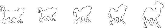
Figure 5. Curve evolution with and without the closedness constraint. Lower and upper bounds for the geodesic distance: 0.462 and 0.464

Figure 6. Curve evolution with and without the closedness constraint. Lower and upper bounds for the geodesic distance: 0.433 and 0.439

Figure 7. Curve evolution with and without the closedness constraint. Lower and upper bounds for the geodesic distance: 0.498 and 0.532

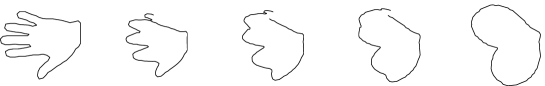
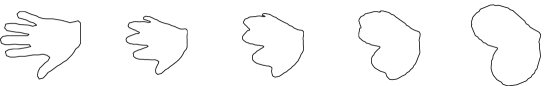
Figure 8. Curve evolution with and without the closedness constraint. Lower and upper bounds for the geodesic distance: 0.513 and 0.528

7. Appendix: The geodesic equation on $G^{\mathrm{imm,scal,1,\infty}}$

7.1. The geodesic equation

We use the method of [11] for the space $\{c\in\operatorname{Imm}_{c}:c(1)=0\}$ which is an open subset in a Fréchet space, with tangent space $\{h\in C^{\infty}(S^{1},\mathbb{C}):f(1)=0\}$. We shall use the following conventions and results from [11]:

$$D_{s}=D_{s,c}=\frac{\partial_{\theta}}{|c_{\theta}|},\quad ds=|c_{\theta}|\,d\theta,\quad D_{c,m}\ell(c)=\int\langle D_{s}m,v_{c}\rangle ds=-\int\kappa_{c}\langle m,n_{c}\rangle\,ds,$$

$$D_{c,m}(D_{s})=-\langle D_{s}m,v_{c}\rangle D_{s},\qquad D_{c,m}(ds)=\langle D_{s}m,v_{c}\rangle ds.$$

Then the derivative of the metric at $c$ in direction $m$ is:

$$D_{c,m}G_{c}(h,k) =\frac{1}{\ell_{c}^{2}}\int\kappa_{c}\langle m,n_{c}\rangle\,ds\cdot\int\langle-D_{s}^{2}h,k\rangle\,ds$$

$$\quad+\frac{1}{\ell_{c}}\int\langle D_{s}m,v_{c}\rangle\langle D_{s}^{2}h,k\rangle\,ds+\frac{1}{\ell_{c}}\int\Big{\langle}D_{s}\Big{(}\langle D_{s}m,v_{c}\rangle D_{s}h\Big{)},k\Big{\rangle}\,ds$$

$$\quad-\frac{1}{\ell_{c}}\int\langle D_{s}^{2}h,k\rangle\langle D_{s}m,v_{c}\rangle\,ds$$

$$=\frac{1}{\ell_{c}^{2}}\int\kappa_{c}\langle m,n_{c}\rangle\,ds\cdot\int\langle-D_{s}^{2}h,k\rangle\,ds$$

$$\quad-\frac{1}{\ell_{c}}\int\Big{\langle}-D_{s}^{2}m,D_{s}^{-1}\Big{(}\langle D_{s}h,D_{s}k\rangle v_{c}\Big{)}\Big{\rangle}\,ds$$

According to [11, 2.1] we should rewrite this as

$$D_{(c,m)}G_{c}(h,k) =G_{c}(K^{n}_{c}(m,h),k)=G_{c}\big{(}m,H^{n}_{c}(h,k)\big{)},$$

and thus we find the two versions $K$ and $H$ of the $G$-gradient of $c\mapsto G_{c}(h,k)$:

$$K_{c}(m,h) =\frac{1}{\ell_{c}}\int\kappa_{c}\langle m,n_{c}\rangle\,ds\cdot h-D_{s}^{-1}\big{(}\langle D_{s}m,v_{c}\rangle D_{s}h\big{)}$$

$$H_{c}(h,k) =-\frac{1}{\ell_{c}}D_{s}^{-2}\big{(}\kappa_{c}n_{c}\big{)}\cdot\int\langle-D_{s}^{2}h,k\rangle\,ds-D_{s}^{-1}\Big{(}\langle D_{s}h,D_{s}k\rangle v_{c}\Big{)}$$

which gives us the geodesic equation by [11, 2.4]:

$$c_{tt} =\tfrac{1}{2}H^{n}_{c}(c_{t},c_{t})-K^{n}_{c}(c_{t},c_{t}).$$

$$=-\tfrac{1}{2}D_{s}^{-2}\big{(}\kappa_{c}n_{c}\big{)}\|c_{t}\|_{G_{c}}^{2}-\tfrac{1}{2}D_{s}^{-1}\big{(}|D_{s}c_{t}|^{2}v_{c}\big{)}$$

(33) $$\quad-\frac{1}{\ell_{c}}\int\kappa_{c}\langle c_{t},n_{c}\rangle\,ds\cdot c_{t}-D_{s}^{-1}\big{(}\langle D_{s}c_{t},v_{c}\rangle D_{s}c_{t}\big{)}$$

7.2 Theorem.

For each $k\geq 3/2$ the geodesic equation derived in 7.1 has unique local solutions in the Sobolev space of $H^{k}$-immersions. The solutions depend $C^{\infty}$ on $t$ and on the initial conditions $c(0,\;.\;)$ and $c_{t}(0,\;.\;)$. The domain of existence (in $t$) is uniform in $k$ and thus this also holds in $\operatorname{Imm}_{*}:=\{c\in\operatorname{Imm}(S^{1},\mathbb{R}^{2}):c(1)=0\}$.

Proof. The proof is very similar to the one of [11, 4.3]. We denote by $*$ any space of based loops $(c(1)=0)$. We consider the geodesic equation as the flow equation of a smooth ($C^{\infty}$) vector field on the $H^{2}$-open set $U^{k}\times H^{k}_{*}(S^{1},\mathbb{R}^{2})$ in the Sobolev space $H^{k}_{*}(S^{1},\mathbb{R}^{2})\times H^{k}_{*}(S^{1},\mathbb{R}^{2})$ where $U^{k}=\{c\in H^{k}_{*}:|c_{\theta}|>0\}\subset H^{k}$ is $H^{2}$-open. To see that this works we will use the following facts: By the Sobolev inequality we have a bounded linear embedding $H^{k}_{*}(S^{1},\mathbb{R}^{2})\subset C^{m}_{*}(S^{1},\mathbb{R}^{2})$ if $k>m+\frac{1}{2}$. The Sobolev space $H^{k}_{*}(S^{1},\mathbb{R})$ is a Banach algebra under pointwise multiplication if $k>\frac{1}{2}$. For any fixed smooth mapping $f$ the mapping $u\mapsto f\circ u$ is smooth $H^{k}_{*}\to H^{k}$ if $k>0$. We write $D_{s,c}:=D_{s}$ just for the remainder of this proof to stress the dependence on $c$. The mapping $(c,u)\mapsto-D_{s,c}^{2}u$ is smooth $U\times H^{k}_{*}\to H^{k-2n}$ and is a bibounded linear isomorphism $H^{k}_{*}\to H^{k-2n}_{*}$ for fixed $c$. This can be seen as follows (compare with [11, 4.5]): It is true if $c$ is parametrized by arclength (look at it in the space of Fourier coefficients). The index is invariant under continuous deformations of elliptic operators of fixed degree, so the index of $-D_{s}^{2}$ is zero in general. But $-D_{s}^{2}$ is self-adjoint positive, so it is injective with vanishing index, thus surjective. By the open mapping theorem it is then bibounded. Moreover $(c,w)\mapsto(-D_{s}^{2})^{-1}(w)$ is smooth $U^{k}\times H^{k-2n}_{*}\to H^{k}_{*}$ (by the inverse function theorem on Banach spaces). The mapping $(c,f)\mapsto D_{s}f=\frac{1}{|c_{\theta}|}\partial_{\theta}f$ is smooth $H^{k}_{*}\times H^{m}_{*}\supset U\times H^{m}_{*}\to H^{m-1}$ for $k\geq m$, and is linear in $f$. We have $v=D_{s,c}c$ and $n=iD_{s,c}c$. The mapping $c\mapsto\kappa(c)$ is smooth on the $H^{2}$-open set $\{c:|c_{\theta}|>0\}\subset H^{k}_{*}$ into $H^{k-2}_{*}$. Keeping all this in mind we now write the geodesic equation 33 as follows:

$$c_{t} =u=:X_{1}(c,u)$$

$$u_{t} =-D_{s,c}^{-2}\Big{(}\tfrac{1}{2}\|u|_{t=0}\|_{G}^{2}.\kappa_{c}.n_{c}+\tfrac{1}{2}D_{s,c}(|D_{s,c}u|^{2}.v_{c})+D_{s,c}(\langle D_{s,c}u,v_{c}\rangle.D_{s,c}u)\Big{)}$$

$$\quad-\Big{(}\frac{1}{\ell_{c}}\int\langle u,D_{s,c}^{2}c\rangle\,ds\Big{)}\Big{|}_{t=0}\cdot u$$

$$=:X_{2}(c,u)$$

Here we used that along any geodesic the norm $\|c_{t}\|_{G}$ and the scaling momentum $-\frac{1}{\ell_{c}}\int\langle c_{t},D_{s,c}^{2}c\rangle\,ds=\partial_{t}\log\ell(c)$ are both constant in $t$. Now a term by term investigation shows that the expression in the brackets is smooth $U^{k}\times H^{k}\to H^{k-2}$ since $k-2>\frac{1}{2}$. The operator $-D_{s,c}^{-2}$ then takes it smoothly back to $H^{k}$. So the vector field $X=(X_{1},X_{2})$ is smooth on $U^{k}\times H^{k}$. Thus the flow $\operatorname{Fl}^{k}$ exists on $H^{k}$ and is smooth in $t$ and the initial conditions for fixed $k$.

Now we consider smooth initial conditions $c_{0}=c(0,\;.\;)$ and $u_{0}=c_{t}(0,\;.\;)=u(0,\;.\;)$ in $C^{\infty}(S^{1},\mathbb{R}^{2})$. Suppose the trajectory $\operatorname{Fl}^{k}_{t}(c_{0},u_{0})$ of $X$ through these intial conditions in $H^{k}$ maximally exists for $t\in(-a_{k},b_{k})$, and the trajectory $\operatorname{Fl}^{k+1}_{t}(c_{0},u_{0})$ in $H^{k+1}$ maximally exists for $t\in(-a_{k+1},b_{k+1})$ with $b_{k+1}<b_{k}$. By uniqueness we have $\operatorname{Fl}^{k+1}_{t}(c_{0},u_{0})=\operatorname{Fl}^{k}_{t}(c_{0},u_{0})$ for $t\in(-a_{k+1,}b_{k+1})$. We now apply $\partial_{\theta}$ to the equation $u_{t}=X_{2}(c,u)=-D_{s,c}^{-2}(\,\dots\,)$, note that the commutator $[\partial_{\theta},-D_{s,c}^{-2}]$ is a pseudo differential operator of order $-2$ again, and write $w=\partial_{\theta}u$. We obtain $w_{t}=\partial_{\theta}u_{t}=-D_{s,c}^{-2}\partial_{\theta}(\,\dots\,)+[\partial_{\theta},-D_{s,c}^{-2}](\,\dots\,)+\text{const}.w$. In the term $\partial_{\theta}(\,\dots\,)$ we consider now only the terms $\partial_{\theta}^{3}u$ and rename them $\partial_{\theta}^{2}w$. Then we get an equation $w_{t}(t,\theta)=\tilde{X}_{2}(t,w(t,\theta))$ which is inhomogeneous bounded linear in $w\in H^{k}$ with coefficients bounded linear operators on $H^{k}$ which are $C^{\infty}$ functions of $c,u\in H^{k}$. These we already know on the intervall $(-a_{k},b_{k})$. This equation therefore has a solution $w(t,\;.\;)$ for all $t$ for which the coefficients exists, thus for all $t\in(a_{k},b_{k})$. The limit $\lim_{t\nearrow b_{k+1}}w(t,\;.\;)$ exists in $H^{k}$ and by continuity it equals $\partial_{\theta}u$ in $H^{k}$ at $t=b_{k+1}$. Thus the $H^{k+1}$-flow was not maximal and can be continued. So $(-a_{k+1},b_{k+1})=(a_{k},b_{k})$. We can iterate this and conclude that the flow of $X$ exists in $\bigcap_{m\geq k}H^{m}=C^{\infty}$. ∎

References

• [1] P. Alexandroff, H Hopf. Topologie. I. Springer-Verlag, Berlin-New York, 1974
• [2] R. Basri, L. Costa, D. Geiger, and D. Jacobs, Determining the similarity of deformable shapes, in IEEE Workshop on Physics based Modeling in Computer Vision, 1995, pp. 135–143.
• [3] R.D. Benguriaand, M. Loss, Connection between the Lieb-Thirring conjecture for Schrödinger operators and an isoperimetric problem for ovals in the plane’, Contemporary Math. 362 (2004), pp.53-61.
• [4] M. P.  Do Carmo, Riemannian Geometry Mathematical Theory and Applications, Birkhäuser, 1992.
• [5] U. Grenander and D. M. Keenan, On the shape of plane images, Siam J. Appl. Math., 53 (1991), pp. 1072–1094.
• [6] S. Helgason, Differential Geometry, Lie Groups and Symmetric Spaces, Graduate Studies in Mathematics, Vol. 34, American Mathematical Society 1978 (revised version 2001).
• [7] E. Klassen, A. Srivastava, W. Mio, and S. Joshi, Analysis of planar shapes using geodesic paths on shape spaces, IEEE Trans. PAMI, (2002).
• [8] A. Kriegl, M. Losik, P.W. Michor, Choosing roots of polynomials smoothly, II, Israel J. Math. 139 (2004), 183-188.
• [9] A. Kriegl, P.W. Michor, The Convenient Setting of Global Analysis, Mathematical Surveys and Monographs, Vol. 53, American Mathematical Society 1997.
• [10] H. Krim and A. Yezzi, eds., Statistics and Analysis of Shapes, Birkhäuser, 2006.
• [11] P. Michor and D. Mumford, An overview of the riemannian metrics on spaces of curves using the hamiltonian approach, Applied and Computational Harmonic Analysis, doi:10.1016/j.acha.2006.07.004.
• [12] W. Mio, A. Srivastava, and S. Joshi, On the shape of plane elastic curves, tech. report, Florida State University, 1995.
• [13] Y. A. Neretin, On jordan angles and the triangle inequality in grassmann manifold, Geometriae Dedicata, 86 (2001).
• [14] B. O’Neill, The fundamental equations of a submersion, Michigan Math. J., (1966), pp. 459–469.
• [15] E. Sharon and D. Mumford, 2d-shape analysis using conformal mapping, in Proceedings IEEE Conference on Computer Vision and Pattern Recognition, 2004.
• [16] A. Trouvé and L. Younes, Diffeomorphic matching in 1d: designing and minimizing matching functionals, in Proceedings of ECCV 2000, D. Vernon, ed., 2000.
• [17] A. Trouvé and L. Younes, On a class of optimal matching problems in 1 dimension, Siam J. Control Opt., vol. 39, number 4, pp 1112-1135, 2001.
• [18] L. Younes, Computable elastic distances between shapes, SIAM J. Appl. Math, 58 (1998), pp. 565–586.
• [19] L. Younes, Optimal matching between shapes via elastic deformations, Image and Vision Computing, (1999).