Non–abelian Reidemeister torsion for twist knots

Abstract.

This paper gives an explicit formula for the $\mathrm{SL}_{\;2}(\mathbb{C})-$non–abelian Reidemeister torsion as defined in [Dub06] in the case of twist knots. For hyperbolic twist knots, we also prove that the non–abelian Reidemeister torsion at the holonomy representation can be expressed as a rational function evaluated at the cusp shape of the knot.

1. Introduction

Twist knots form a family of special two–bridge knots which include the trefoil knot and the figure eight knot. The knot group of a two–bridge knot has a particularly nice presentation with only two generators and a single relation. One could find our interest in this family of knots in the following facts: first, twist knots except the trefoil knot are hyperbolic; and second, twist knots are not fibered except the trefoil knot and the figure eight knot (see Remark 2 of the present paper for details).

The non–abelian Reidemeister torsion associated to a representation of a knot group to a general linear group over a field has been studied since the early 1990’s. It was initially considered as a twisted Alexander polynomial by Lin [Lin01], Wada [Wad94], and later interpreted as a form of Reidemeister torsion by Kitano [Kit96], Kirk-Livingston [KL99] and Goda–Kitano and Morifuji [GKM05]. This invariant in many cases is stronger than the classical ones, for example it detects the unknot [SW06], and decides fiberness for knots of genus one [FV07]. Abelian Reidemeister torsions are now well–known, see e.g. Turaev’s monograph [Tur02]; but unfortunately in the case of non–abelian representations concrete computations of such torsions are still very few. In [Por97], Porti began the study of the non–abelian Reidemeister torsion (consider as a functional on the non–abelian part of the character variety) with the adjoint representation associated to an irreducible representation of the fundamental group of a hyperbolic three–dimensional manifold to ${\mathrm{SL}_{2}({\mathbb{C}})}$. In [Dub05], the first author introduced a sign–refined version of this torsion. In the present paper, we call this (sign–refined) torsion the ${\mathrm{SL}_{2}({\mathbb{C}})}-$non–abelian Reidemeister torsion. One can observe that this torsion has connections with hyperbolic structures, the theory of character variety, and the theory of Chern-Simons invariant, see e.g. [DK07].

In [Dub06, Main Theorem], one can find an “explicit”  formula which gives the value of the non–abelian Reidemeister torsion for fibered knots in terms of the map induced by the monodromy of the knot at the level of the character variety of the knot exterior. In particular, a practical formula of the non–abelian Reidemeister torsion for torus knots is presented in [Dub06, Section 6.2]. One can also find an explicit formula for the non–abelian Reidemeister torsion for the figure eight knot in [Dub06, Section 7]. More recently, the last author found [Yam05, Theorem 3.1.2] an interpretation of the non–abelian Reidemeister torsion in terms of a sort of twisted Alexander polynomial (called in this paper, the non–abelian Reidemeister torsion polynomial) and gave an explicit formula of the non–abelian torsion for the twist knot $5_{2}$.

In the present paper we give an explicit formula of the non–abelian Reidemeister torsion for all twist knots. Since twist knots are particular two–bridge knots, this paper is a first step in the understanding of the non–abelian Reidemeister torsion for two–bridge knots.

Organization

The outline of the paper is as follows. We recall some properties of twist knots in Section 2. In Section 3, we give a review of the character variety of twist knots including remarks on parabolic representations and Riley’s method for describing the non–abelian part of the character variety. Next we give an explicit formula for the cusp shape of hyperbolic twist knots. In Section 4, we recall the definition of the non–abelian Reidemeister torsion for a knot and an algebraic description of this invariant. We give formulas for the non–abelian Reidemeister torsion for twist knots in Section 5. In particular, we show in Subsection 5.3 that the non–abelian Reidemeister torsion for a hyperbolic twist knot at its holonomy representation is expressed by using the cusp shape of the hyperbolic structure of the knot complement. The last part of the paper (Subsection 5.4) deals with some remarks on the behavior of the sequence of non–abelian Reidemeister torsions for twist knots at the holonomy indexed by the number of crossings. The appendix contains concrete examples and tables of the values of the non–abelian torsion for some explicit twist knots.

2. Twist knots

Notation.

According to the notation of [HS04], the twist knots are written $J(\pm 2,n)$, where $n$ is an integer. The $n$ crossings are right–handed when $n>0$ and left–handed when $n<0$.

Figure 1. The diagrams of $J(2,n)$ and $J(-2,n)$, $n>0$.

Here are some important facts about twist knots.

1. By definition, if $n\in\{0,1\}$ then $J(2,n)$ and $J(-2,-n)$ are the unknot. Also observe that $J(2,-1)$ and $J(-2,1)$ are isotopic to $J(-2,-2)$ and $J(2,2)$ respectively (for general cases, see below). For this reason, in all this paper, we focus on the knots $J(\pm 2,n)$ with $|n|\geqslant 2$.

2. If we rotate the diagram of $J(2,n)$ by a 90 degrees angle clockwise then we get a diagram of a rational knot in the sense of Conway. In rational knot notation $J(2,n)$, $n>0$, is represented by the continued fraction $[n,-2]=\frac{1}{-2+1/n}=\frac{-n}{2n-1}.$ Therefore in two–bridge knot notation, for $n>0$ we have $J(2,n)=b(2n-1,-n)=b(2n-1,n-1).$

   Similarly, the knot $J(2,-n)$, $n>0$, is represented by the continued fraction $[-n,-2]$, therefore $J(2,-n)=b(2n+1,n+1).$ On the other hand, the knot $J(-2,n)$, $n>0$, is $b(2n+1,n)$ and $J(-2,-n)$, $n>0$, is $b(2n-1,n)$.

3. Two other important observations are the following:

   • the twist knot $J(2,n)$ is isotopic to $J(-2,n-1)$ (see [HS04]),

   • and $J(-2,-n)$ is the mirror image of $J(2,n)$.

As a consequence, we will only consider the twist knots $J(2,n)$, where $n$ is an integer such that $|n|\geqslant 2$. From now on, we adopt in the sequel the following terminology: a twist knot $J(2,n)$ is said to be even (resp. odd) if $n$ is even (resp. odd).

Example.

Note that in Rolfsen’s table [Rol90], the trefoil knot $3_{1}=J(2,2)=b(3,1)$, the figure eight knot $4_{1}=J(2,-2)=b(5,3)$, $5_{2}=J(2,4)$ and $6_{1}=J(2,-4)$ etc.

Notation.

For a knot $K$ in $S^{3}$, we let $E_{K}$ (resp. $\Pi(K)$) denote the exterior (resp. the group) of $K$, i.e. $E_{K}=S^{3}\setminus N(K)$, where $N(K)$ is an open tubular neighborhood of $K$ (resp. $\Pi(K)=\pi_{1}(E_{K})$).

Convention.

Suppose that $S^{3}$ is oriented. The exterior of a knot is thus oriented and we know that it is bounded by a $2$-dimensional torus $T^{2}$. This boundary inherits an orientation by the convention “the inward pointing normal vector in the last position”. Let $\mathrm{int}(\cdot,\cdot)$ be the intersection form on the boundary torus induced by its orientation. The peripheral subgroup $\pi_{1}(T^{2})$ is generated by the meridian–longitude system $(\mu,\lambda)$ of the knot. If we suppose that the knot is oriented, then $\mu$ is oriented by the convention that the linking number of the knot with $\mu$ is $+1$. Next, $\lambda$ is the oriented preferred longitude using the rule $\mathrm{int}(\mu,\lambda)=+1$. These orientation conventions will be used in the definition of the (sign–refined) twisted Reidemeister torsion.

Twist knots live in the more general family of two-bridge knots. The group of such a knot admits a particularly nice Wirtinger presentation with only two generators and a single relation. Such Wirtinger presentations of groups of twist knots are given in the two following facts (see for example [Rol90] or [HS04] for a proof). We distinguish even and odd cases and suppose that $m\in{\mathbb{Z}}$.

Fact 1.

The knot group of $J(2,2m)$ admits the following presentation:

(1) $$\Pi(J(2,2m))=\langle x,y\,|\,w^{m}x=yw^{m}\rangle$$

where $w$ is the word $[y,x^{-1}]=yx^{-1}y^{-1}x$.

Fact 2.

The knot group of $J(2,2m+1)$ admits the following presentation:

(2) $$\Pi(J(2,2m+1))=\langle x,y\,|\,w^{m}x=yw^{m}\rangle$$

where $w$ is the word $[x,y^{-1}]=xy^{-1}x^{-1}y$.

One can easily describe the peripheral–system $(\mu,\lambda)$ of a twist knot. It is expressed in the knot group as:

$$\mu=x\text{ and }\lambda=(\stackrel{{\scriptstyle\leftarrow}}{{w}})^{m}w^{m},$$

where we let $\stackrel{{\scriptstyle\leftarrow}}{{w}}$ denote the word obtained from $w$ by reversing the order of the letters.

Remark 1.

The knot group of a two–bridge knot $K$ admits a distinguished Wirtinger presentation of the following form:

$$\Pi(K)=\left\langle{x,y\,|\,\Omega x=y\Omega}\right\rangle\text{ where }\Omega=x^{\epsilon_{1}}y^{\epsilon_{n}}x^{\epsilon_{2}}y^{\epsilon_{n-1}}\dotsb x^{\epsilon_{n}}y^{\epsilon_{1}},\text{ with }\epsilon_{i}=\pm 1.$$

With the above notation, for $K=J(2,2m)$, $m\in{\mathbb{Z}}\setminus\{0\}$, the word $\Omega$ is:

(3) $$\Omega_{m}=\begin{cases}w^{m}&\text{ if }m<0,\\ x^{-1}{(\overline{w})}^{m-1}y^{-1}&\text{ if }m>0.\end{cases}$$

Here $\overline{w}={(\stackrel{{\scriptstyle\leftarrow}}{{w}})}^{-1}$, i.e. the word $\overline{w}$ is obtain from $w$ by changing each of its letters by its reverse. Of course this choice is strictly equivalent to presentation (1). But in a sense, when $m>0$ the word $w^{m}$ does not give a “reduced” relation (some cancelations are possible in $w^{m}xw^{-m}y^{-1}$) which is not the case for the word $\Omega_{m}$.

Some more elementary properties of twist knots are discussed in the following remark.

Remark 2.

1. The knot groups $\Pi(J(2,2m+1))$ and $\Pi(J(2,-2m))$ are isomorphic by interchanging $x$ and $y$. Algebraically, it is thus enough to consider the case of even twist knots (see in particular Remark 13).

2. The genus of a twist knot is $1$ ([Ada94, p. 99]). Thus, the only torus knot which is a twist knot is the trefoil knot $3_{1}$.

3. Twist knots are hyperbolic knots except the trefoil knot (see for example [Men84]).

4. It is well known (see for example [Rol90]) that the Alexander polynomial of the twist knot $J(2,2m)$ is given by $\Delta_{J(2,2m)}(t)=mt^{2}+(1-2m)t+m.$ Moreover, using the mirror image invariance of the Alexander polynomial, one has $\Delta_{J(2,2m+1)}(t)=\Delta_{J(2,-2m)}(t)$. Thus the Alexander polynomial becomes monic if and only if $m$ is $\pm 1$. As a consequence, the knot $J(2,2m)$ is not fibered (since its Alexander polynomial is not monic) except for $m=\pm 1$, that is to say except for the trefoil knot and the figure eight knot, which are known to be fibered knots.

   

   Figure 2. The Whitehead link.

5. Twist knot exteriors can be obtained by surgery on the trivial component of the Whitehead link $\mathcal{W}$ (see Fig. 2). More precisely, $E_{J(2,-2m)}=\mathcal{W}({1/m})$ is obtained by a surgery of slope $1/m$ on the trivial component of the Whitehead link $\mathcal{W}$, see [Rol90, p. 263] for a proof. As a consequence, twist knots are all virtually fibered (a manifold $M$ is said to be virtually fibered if there is a finite cover of $M$ that is fibered), see [Lei02].

3. On the ${\mathrm{SL}_{2}({\mathbb{C}})}$-character variety and non–abelian representations

3.1. Review on the ${\mathrm{SL}_{2}({\mathbb{C}})}$-character variety of knot groups

Given a finitely generated group $\pi$, we let

$$R(\pi;{\mathrm{SL}_{2}({\mathbb{C}})})=\mathrm{Hom}(\pi;{\mathrm{SL}_{2}({\mathbb{C}})})$$

denote the space of ${\mathrm{SL}_{2}({\mathbb{C}})}$-representations of $\pi$. As usual, this space is endowed with the compact–open topology. Here $\pi$ is assumed to have the discrete topology and the Lie group ${\mathrm{SL}_{2}({\mathbb{C}})}$ is endowed with the usual one.

A representation $\rho\colon\pi\to{\mathrm{SL}_{2}({\mathbb{C}})}$ is called abelian if $\rho(\pi)$ is an abelian subgroup of ${\mathrm{SL}_{2}({\mathbb{C}})}$. A representation $\rho$ is called reducible if there exists a proper subspace $U\subset{\mathbb{C}}^{2}$ such that $\rho(g)(U)\subset U$, for all $g\in\pi$. Of course, any abelian representation is reducible (while the converse is false in general). A representation is called irreducible if it is not reducible.

The group ${\mathrm{SL}_{2}({\mathbb{C}})}$ acts on the representation space $R(\pi;{\mathrm{SL}_{2}({\mathbb{C}})})$ by conjugation, but the naive quotient $R(\pi;{\mathrm{SL}_{2}({\mathbb{C}})})/{\mathrm{SL}_{2}({\mathbb{C}})}$ is not Hausdorff in general. Following [CS83], we will focus on the character variety $X(\pi)=X(\pi;{\mathrm{SL}_{2}({\mathbb{C}})})$ which is the set of characters of $\pi$. Associated to the representation $\rho\in R(\pi;{\mathrm{SL}_{2}({\mathbb{C}})})$, its character $\chi_{\rho}\colon\pi\to{\mathbb{C}}$ is defined by $\chi_{\rho}(g)=\mathrm{tr}(\rho(g))$, where $\mathrm{tr}$ denotes the trace of matrices. In some sense $X(\pi)$ is the “algebraic quotient”  of $R(\pi;{\mathrm{SL}_{2}({\mathbb{C}})})$ by the action by conjugation of ${\mathrm{PSL}_{2}({\mathbb{C}})}$. It is well known that $R(\pi,{\mathrm{SL}_{2}({\mathbb{C}})})$ and $X(\pi)$ have the structure of complex algebraic affine varieties (see [CS83]).

Let ${R}^{\mathrm{irr}}(\pi;{\mathrm{SL}_{2}({\mathbb{C}})})$ denote the subset of irreducible representations of $\pi$, and $X^{\mathrm{irr}}(\pi)$ denote its image under the map ${R}(\pi;{\mathrm{SL}_{2}({\mathbb{C}})})\to X(\pi)$. Note that two irreducible representations of $\pi$ in ${\mathrm{SL}_{2}({\mathbb{C}})}$ with the same character are conjugate by an element of ${\mathrm{SL}_{2}({\mathbb{C}})}$, see [CS83, Proposition 1.5.2]. Similarly, we write $X^{\mathrm{nab}}(\Pi(K))$ for the image of the set $R^{\mathrm{nab}}(\Pi(K))$ of non–abelian representations in $X(\Pi(K))$. Note that $X^{\mathrm{irr}}(\Pi(K))\subset X^{\mathrm{nab}}(\Pi(K))$ and observe that this inclusion is strict in general.

3.2. Review on the character varieties of two–bridge knots

Here we briefly review Riley’s method [Ril84] for describing the non–abelian part of the representation space of two–bridge knot groups.

The knot group of a two–bridge knot $K$ admits a presentation of the following form:

(4) $$\Pi(K)=\left\langle{x,y\,|\,\Omega x=y\Omega}\right\rangle\text{ where }\Omega=x^{\epsilon_{1}}y^{\epsilon_{n}}x^{\epsilon_{2}}y^{\epsilon_{n-1}}\dotsb x^{\epsilon_{n}}y^{\epsilon_{1}},\;\epsilon_{i}=\pm 1.$$

We consider the following matrices: $C_{1}=\begin{pmatrix}\sqrt{s}&1\\ 0&{1}/{\sqrt{s}}\end{pmatrix},\ D_{1}=\begin{pmatrix}\hphantom{-}\sqrt{s}&0\\ -u&{1}/{\sqrt{s}}\end{pmatrix};$ and $C_{2}=\begin{pmatrix}\sqrt{s}&{1}/{\sqrt{s}}\\ 0&{1}/{\sqrt{s}}\end{pmatrix},\ D_{2}=\begin{pmatrix}\hphantom{-t}\sqrt{s}&0\\ -\sqrt{s}u&{1}/{\sqrt{s}}\end{pmatrix};$ where $s\in{\mathbb{C}}^{*}$, $\sqrt{s}$ is some square root, and $u\in{\mathbb{C}}$.

Remark 3.

Note that $C_{2}$ and $D_{2}$ are respectively conjugate to $C_{1}$ and $D_{1}$ via $U=\bigl{(}\begin{smallmatrix}s^{-1/4}&0\\ 0&s^{1/4}\end{smallmatrix}\bigr{)}$.

For a two–bridge knot $K$, $x$ and $y$ are conjugate elements in $\Pi(K)$ and represent meridians of the knot, therefore $\rho(x)$ and $\rho(y)$ have same traces. If $\rho(x)$ and $\rho(y)$ do not commute, i.e. if $\rho$ is non–abelian, then up to a conjugation one can assume that $\rho(x)$ and $\rho(y)$ are the matrices $C_{1}$ and $D_{1}$ respectively. With this notation, we have the following result due to Riley [Ril84].

Proposition 3.

The homomorphism $\rho\colon\Pi(K)\to\mathrm{SL}_{2}({\mathbb{C}})$ defined by $\rho(x)=C_{1}$ and $\rho(y)=D_{1}$ is a non–abelian representation of $\Pi(K)$ if and only if the pair $(s,u)\in{\mathbb{C}}^{2}$ satisfies the following equation:

(5) $$w_{1,1}+({1}/{\sqrt{s}}-\sqrt{s})w_{1,2}=0$$

where $W=\rho(\Omega)$.

Conversely, every non–abelian representation is conjugated to a representation satisfying Eq. (5).

Remark 4.

Similarly, if $\rho(x)=C_{2}$ and $\rho(y)=D_{2}$, then Riley’s equation is

(6) $$w_{1,1}+(1-s)w_{1,2}=0.$$

Notation 1.

We let $\phi_{K}(s,u)=w_{1,1}+(1-s)w_{1,2}$ denote the left hand side of Eq. $(\ref{eq:R_alternative})$ and call it the Riley polynomial of $K$.

3.3. The holonomy representation of a hyperbolic twist knot

3.3.1. Some generalities

It is well known that the complete hyperbolic structure of a hyperbolic knot complement determines a unique discrete faithful representation of the knot group in $\mathrm{PSL}_{2}({\mathbb{C}})$, called the holonomy representation. It is proved [Sha02, Proposition 1.6.1] that such a representation lifts to ${\mathrm{SL}_{2}({\mathbb{C}})}$ and determines two irreducible representations in ${\mathrm{SL}_{2}({\mathbb{C}})}$.

The trace of the peripheral–system at the holonomy is $\pm 2$ because their images by the holonomy are parabolic matrices. More precisely, Calegari [Cal06] proved that the trace of the longitude at the holonomy is always $-2$ and the trace of the meridian at the holonomy is $\pm 2$, depending on the choice of the lift. We summarize all this in the following important fact.

Fact 4.

Let $\rho_{0}$ be one of the two lifts of the discrete and faithful representation associated to the complete hyperbolic structure of a hyperbolic knot $K$ and let $T^{2}=\partial E_{K}$ denote the boundary of the knot exterior. The restriction of $\rho_{0}$ to $\pi_{1}(T^{2})$ is conjugate to the parabolic representation such that

$$\mu\mapsto\pm\left(\begin{array}[]{cc}1&1\\ 0&1\end{array}\right),\quad\lambda\mapsto\left(\begin{array}[]{cc}-1&\hphantom{-}{\mathfrak{c}}\\ \hphantom{-}0&-1\end{array}\right).$$

Here ${\mathfrak{c}}={\mathfrak{c}}(\lambda,\mu)\in{\mathbb{C}}$ is called the cusp shape of $K$.

Remark 5.

The universal cover of the exterior of a hyperbolic knot is the hyperbolic $3$-space $\mathbb{H}^{3}$. The cusp shape can be seen as the ratio of the translations of the parabolic isometries of $\mathbb{H}^{3}$ induced by projections to $\mathrm{PSL}_{2}({\mathbb{C}})$. Of course, the cusp shape ${\mathfrak{c}}={\mathfrak{c}}(\lambda,\mu)$ depends on the choice of the basis $(\mu,\lambda)$ for $\pi_{1}(T^{2})$. A change in the basis of $\pi_{1}(T^{2})$ shifts ${\mathfrak{c}}$ by an integral Möbius transformation.

3.3.2. Holonomy representations of twist knots

This subsection is concerned with the ${\mathrm{SL}_{2}({\mathbb{C}})}$-representations which are lifts of the holonomy representation in the special case of (hyperbolic) twist knots. In particular, we want to specify the images, up to conjugation, of the group generators $x$ and $y$ (see the group presentation (4)).

Lemma 5.

Let $K$ be a hyperbolic two–bridge knot and suppose that its knot group admits the following presentation $\Pi(K)=\langle x,y\,|\,\Omega x=y\Omega\rangle$. If $\rho_{0}$ denotes a lift in ${\mathrm{SL}_{2}({\mathbb{C}})}$ of the holonomy representation, then $\rho_{0}$ is given, up to conjugation, by

$$x\mapsto\pm\left(\begin{array}[]{cc}1&1\\ 0&1\end{array}\right),\quad y\mapsto\pm\left(\begin{array}[]{cc}\hphantom{-}1&0\\ -u&1\end{array}\right),$$

where $u$ is a root of Riley’s equation $\phi_{K}(1,u)=0$ of $K$.

Proof.

It follows from Fact 4 that each lift of the holonomy representation maps the meridian to $\pm\left(\begin{smallmatrix}1&1\\ 0&1\end{smallmatrix}\right).$ It is known that the lifts of the holonomy representation are irreducible ${\mathrm{SL}_{2}({\mathbb{C}})}$-representations, in particular, non–abelian ones. Hence we can construct the ${\mathrm{SL}_{2}({\mathbb{C}})}$-representations which are conjugate to the lifts of the holonomy representation by using roots of Riley’s equation. Using Section 3.2, if $x$ is sent to $\pm\left(\begin{smallmatrix}1&1\\ 0&1\end{smallmatrix}\right)$ then $y$ is sent to $\pm\left(\begin{smallmatrix}\hphantom{-}1&0\\ -u&1\end{smallmatrix}\right)$, where $u$ is a root of Riley’s equation $\phi_{K}(1,u)=0$. ∎

Notation.

If we let $A$ be an element of ${\mathrm{SL}_{2}({\mathbb{C}})}$, then the adjoint actions of $A$ and $-A$ are same. So, we use the ${\mathrm{SL}_{2}({\mathbb{C}})}$-representation such that

$$x\mapsto\left(\begin{array}[]{cc}1&1\\ 0&1\end{array}\right),\quad y\mapsto\left(\begin{array}[]{cc}\hphantom{-}1&0\\ -u&1\end{array}\right)\quad(\text{where }u\text{ is such that }\phi_{K}(1,u)=0)$$

as a lift of the holonomy representation and we improperly call it the holonomy representation.

3.4. On parabolic representations of twist knot groups

In this subsection, we are interested in the parabolic representations of (hyperbolic) two–bridge knot groups and especially twist knot groups. The holonomy representation is one of them. Lemma 5 characterizes the holonomy representation algebraically and says that it corresponds to a root of Riley’s equation $\phi_{K}(1,u)=0$. A natural and interesting question is the following: which roots of Riley’s equation $\phi_{K}(1,u)=0$ correspond to the holonomy representation? Here we will give a geometric characterization of such roots in the case of two–bridge knots.

3.4.1. Remarks

We begin this section by some elementary but important remarks on the roots of Riley’s equation $\phi_{K}(1,u)=0$ corresponding to holonomy representations.

1. One can first notice that such roots are necessarily complex numbers which are not real, because the discrete and faithful representation is irreducible and not conjugate to a real representation (i.e. a representation such that the image of each element is a matrix with real entries).

2. One can also observe that holonomy representations correspond to a pair of complex conjugate roots of Riley’s equation $\phi_{K}(1,u)=0$ as it is easy to see.

3.4.2. Generalities: the case of two–bridge knots

Let $K$ be a hyperbolic two–bridge knot. Suppose that a presentation of the knot group $\Pi(K)$ is given as in Eq. (4) by

$$\Pi(K)=\langle{x,y\,|\,\Omega x=y\Omega}\rangle,\text{ where }\Omega\text{ is a word in }x,y.$$

The longitude of $K$ is of the form: $\lambda=\stackrel{{\scriptstyle\leftarrow}}{{\Omega}}\Omega\,x^{n}$. Here $n$ is an integer such that the sum of the exponents in the word $\lambda$ is $0$ and we repeat that $\stackrel{{\scriptstyle\leftarrow}}{{\Omega}}$ denotes the word obtained from $\Omega$ by reversing the order of the letters.

Let $\rho\colon\Pi(K)\to{\mathrm{SL}_{2}({\mathbb{C}})}$ be a representation such that:

$$x\mapsto\pm\left(\begin{array}[]{cc}1&1\\ 0&1\end{array}\right),\quad y\mapsto\pm\left(\begin{array}[]{cc}1&0\\ -u&1\end{array}\right)$$

where $u$ is necessarily a root of Riley’s equation $\phi_{K}(1,u)=0$. Suppose that

$$\rho(\Omega)=\left(\begin{array}[]{cc}w_{1,1}&w_{1,2}\\ w_{2,1}&w_{2,2}\end{array}\right)$$

where $w_{i,j}$ is a polynomial in $u$ for all $i,j\in\{1,2\}$.

Riley’s method gives us the following identities (see Section 3.2):

$$w_{1,1}=0\text{ and }uw_{1,2}+w_{2,1}=0.$$

Thus

$$\rho(\Omega)=\left(\begin{array}[]{cc}0&w_{1,2}\\ -uw_{1,2}&w_{2,2}\end{array}\right).$$

The fact that $\rho(w)\in{\mathrm{SL}_{2}({\mathbb{C}})}$ further gives the following equation:

(7) $$uw_{1,2}^{2}=1.$$

The crucial point for computing $\rho(\lambda)$ is to express $\rho(\stackrel{{\scriptstyle\leftarrow}}{{\Omega}})$ with the help of $\rho(\Omega)$. Consider the diagonal matrix:

$$\mathbf{i}=\left(\begin{array}[]{cc}i&0\\ 0&-i\end{array}\right)\in{\mathrm{SL}_{2}({\mathbb{C}})},$$

where $i$ stands for a square root of $-1$. Let $Ad$ denote the adjoint representation of the Lie group ${\mathrm{SL}_{2}({\mathbb{C}})}$. Then the following identities hold:

$$\rho(x^{-1})=Ad_{\mathbf{i}}(\rho(x)),\;\rho(y^{-1})=Ad_{\mathbf{i}}(\rho(y))\text{ and }\rho(\Omega^{-1})=Ad_{\mathbf{i}}(\rho(\stackrel{{\scriptstyle\leftarrow}}{{\Omega}})).$$

Thus, we have

$$\rho(\stackrel{{\scriptstyle\leftarrow}}{{\Omega}})=Ad_{\mathbf{i}}(\rho({\Omega}^{-1}))=\left(\begin{array}[]{cc}w_{2,2}&w_{1,2}\\ w_{2,1}&w_{1,1}\end{array}\right).$$

Next, a direct computation gives:

(8) $$\rho(\lambda)=\rho(\stackrel{{\scriptstyle\leftarrow}}{{\Omega}})\rho(\Omega)\rho(x)^{n}=\left(\begin{array}[]{cc}-uw^{2}_{1,2}&-nuw^{2}_{1,2}+2w_{1,2}w_{2,2}\\ 0&-uw^{2}_{1,2}\end{array}\right).$$

Combining Eqs. (7) and (8), we obtain

(9) $$\rho(\lambda)=\left(\begin{array}[]{cc}-1&-n+2w_{1,2}w_{2,2}\\ 0&-1\end{array}\right).$$

And we conclude that the cusp shape of $K$ is

(10) $${\mathfrak{c}}=n-2w_{1,2}w_{2,2}.$$

Remark 6.

In particular, Eq. (9) gives us, by an elementary and direct computation, Calegari’s result [Cal06]: $\mathrm{tr}\,\rho_{0}(\lambda)=-2$ for the discrete faithful representation $\rho_{0}$ associated to the complete hyperbolic structure of the exterior of a (hyperbolic) two–bridge knot.

3.4.3. The special case of twist knots

In the case of hyperbolic twist knots, we can further estimate $w_{i,j}$ in Eq. (10). In fact, we only consider the case where $K=J(2,2m)$ in what follows. The group $\Pi(K)$ of such a knot has the following presentation:

$$\Pi(K)=\langle{x,y\,|\,w^{m}x=yw^{m}}\rangle,$$

where $w$ is the commutator $[y,x^{-1}]$ (see Fact 1, Section 2). A direct computation of the commutator $\rho(w)=[\rho(y),\rho(x)^{-1}]$ gives:

$$W=\rho(w)=\left(\begin{array}[]{cc}1-u&-u\\ u^{2}&u^{2}+u+1\end{array}\right)\quad(\text{where }u\text{ is such that }\phi_{K}(1,u)=0).$$

Using the Cayley–Hamilton identity, it is easy to obtain the following recursive formula for the powers of the matrix $W$:

(11) $$W^{k}-(u^{2}+2)W^{k-1}+W^{k-2}=0,\;k\geqslant 2.$$

Eq. (11) implies, by induction on $k$,

$$w_{2,2}=-(u+2)w_{1,2}.$$

Since $n=0$ and $uw_{1,2}^{2}=1$, the cusp shape of the twist knot $K$ is:

$${\mathfrak{c}}=n+(2u+4)w_{1,2}^{2}=\frac{2u+4}{u}.$$

In other words, the root $u_{0}$ of Riley’s equation $\phi_{K}(1,u)=0$ corresponding to the holonomy representation satisfies the following equation:

(12) $$u_{0}=\frac{4}{{\mathfrak{c}}-2},$$

where ${\mathfrak{c}}$ is the cusp shape of the knot exterior.

Remark 7.

Eq. (12) gives a geometric characterization of the (pair of complex conjugate) roots of Riley’s equation $\phi_{K}(1,u)=0$ associated to the holonomy representation in terms of the cusp shape, a geometric quantity associated to each cusped hyperbolic $3$-dimensional manifold.

3.5. The character varieties of twist knots: a recursive description

T. Le [Le94] gives a recursive description of the ${\mathrm{SL}_{2}({\mathbb{C}})}$-character variety of two–bridge knots and apply it to obtain an explicit description of the ${\mathrm{SL}_{2}({\mathbb{C}})}$-character variety of torus knots. Here we apply his method to obtain an explicit recurrent description of the ${\mathrm{SL}_{2}({\mathbb{C}})}$-character variety of twist knots. This is the main difference with the description given by Hoste and Shanahan [HS04].

Let $n=2m$ or $2m+1$, recall that $\Pi(J(2,n))=\langle x,y\,|\,\Omega_{m}x=y\Omega_{m}\rangle,$ where $\Omega_{m}$ is a word in $x,y$ (see Facts 1–2).

Notation.

Let $\gamma\in\Pi(J(2,n))$. Following a notation introduced in [CGLS87], we let

$$I_{\gamma}:X(\Pi(J(2,n)))\to{\mathbb{C}}$$

be the trace–function defined by $I_{\gamma}:\rho\mapsto\mathop{\mathrm{tr}}\nolimits(\rho(\gamma))$.

Let $a=I_{x}$, $b=I_{xy}$ and recall the following useful formulas for $A,B,C\in{\mathrm{SL}_{2}({\mathbb{C}})}$:

(13) $$\mathrm{tr}(A^{-1})=\mathrm{tr}(A)\text{ and }\mathrm{tr}(AB)=\mathrm{tr}(BA),$$

(14) $$\mathrm{tr}(AB)+\mathrm{tr}(A^{-1}B)=\mathrm{tr}(A)\mathrm{tr}(B),$$

(15) $$\mathrm{tr}(ABA^{-1}B^{-1})=-2-\mathrm{tr}(A)\mathrm{tr}(B)\mathrm{tr}(AB)+(\mathrm{tr}(A))^{2}+(\mathrm{tr}(B))^{2}+(\mathrm{tr}(AB))^{2}.$$

As $x$ and $y$ are conjugate elements in $\Pi(J(2,n))$, we have $I_{y}=a=I_{x}$. If $\gamma$ is a word in the letters $x$ and $y$, then $I_{\gamma}$ can always be expressed as a polynomial function in $a$ and $b$. For example, combining the usual Formulas (13), (14) and (15), one can easily observe that for $w=[y,x^{-1}]=yx^{-1}y^{-1}x$, we have

(16) $$I_{w}=-2-a^{2}b+2a^{2}+b^{2}.$$

The character variety of $\Pi(J(2,n))$ is thus parametrized by $a$ and $b$. Here is a practical description of it:

1. We first consider the abelian part of the character variety. It is easy to see that the equation $a^{2}-b-2=0$ determines the abelian part of the character variety of any knot group.

2. Next, consider the non-abelian part of the character variety of $\Pi(J(2,n))$, suppose that the length of the word $\Omega_{m}$ is $2k+2$ (we know that the length of $\Omega_{m}$ is even). According to [Le94, Theorem 3.3.1], the non–abelian part of the character variety of $\Pi(J(2,n))$, for $n=2m$ or $2m+1$, is determined by the polynomial equation:

   $${\mathbf{\Phi}}_{m}(a,b)=0,$$

   where

   $${\mathbf{\Phi}}_{m}(a,b)=I_{\Omega_{m}}-I_{\Omega_{m}^{\prime}}+\dotsb+(-1)^{k}I_{\Omega_{m}^{(k)}}+(-1)^{k+1}.$$

   Here we adopt the following notation: if $\Lambda$ is a word then $\Lambda^{\prime}$ denotes the word obtained from $\Lambda$ by deleting the two end letters.

Let us give the two simplest examples to illustrate this general result and find again some well–known facts.

Example 1.

The trefoil knot $3_{1}$ is the twist knot $J(2,2)$. With the above notation, one has $\Omega_{1}=x^{-1}y^{-1}$. Thus applying Le’s method, the non–abelian part of the character variety is given by the polynomial equation:

$${\mathbf{\Phi}}_{1}(a,b)=I_{x^{-1}y^{-1}}-1=0,$$

which reduces to

$$b=1.$$

Example 2.

The figure eight knot $4_{1}$ is the twist knot $J(2,-2)$. With the above notation, one has $\Omega_{-1}=x^{-1}yxy^{-1}$. Thus, the non–abelian part of the character variety of the group of the figure eight knot is given by the polynomial equation:

$${\mathbf{\Phi}}_{-1}(a,b)=I_{x^{-1}yxy^{-1}}-I_{yx}+1=0,$$

which reduces, using Equation (16), to:

$$2a^{2}+b^{2}-a^{2}b-b=1.$$

Now, we turn back to the general case and only consider the twist knot $J(2,2m)$ (see Item (2) of Remark 2). Recall that (see Remark 1):

(17) $$\Pi(J(2,2m))=\langle x,y\;|\;\Omega_{m}x=y\Omega_{m}\rangle,\text{ where }\Omega_{m}=\begin{cases}w^{m}&\text{ if }m<0,\\ x^{-1}{(\overline{w})}^{m-1}y^{-1}&\text{ if }m>0.\end{cases}$$

Here $w=[y,x^{-1}]$ and $\overline{w}=[y^{-1},x]$ and observe that the length of the word $\Omega_{m}$ is $4m$, if $m<0$, and $4m-2$, if $m>0$.

Our method is based on the fact that the word $\Omega_{m}$ in the distinguished Wirtinger presentation (17) of $\Pi(J(2,2m))$ presents a particularly nice “periodic” property. This property is discussed in the following obvious claim.

Claim 6.

For $m\in{\mathbb{Z}}^{*}$, we have

$$\Omega_{m}^{(4)}=\begin{cases}w^{m+2}&\text{ if }m\leqslant-2,\\ x^{-1}{(\overline{w})}^{m-3}y^{-1}&\text{ if }m\geqslant 3.\end{cases}$$

Based on Claim 6, for $m\geqslant 0$, we adopt the following notation:

$$S^{+}_{m}=I_{\Omega_{m+2}},\;T^{+}_{m}=I_{{(\Omega_{m+2})}^{\prime}},\;U^{+}_{m}=I_{{(\Omega_{m+2})}^{\prime\prime}}\text{ and }V^{+}_{m}=I_{{(\Omega_{m+2})}^{\prime\prime\prime}},$$

and similarly, for $m\leqslant 0$,

$$S^{-}_{m}=I_{\Omega_{m-2}},\;T^{-}_{m}=I_{{(\Omega_{m-2})}^{\prime}},\;U^{-}_{m}=I_{{(\Omega_{m-2})}^{\prime\prime}}\text{ and }V^{-}_{m}=I_{{(\Omega_{m-2})}^{\prime\prime\prime}}.$$

The Cayley–Hamilton identity applied to the matrix $A^{2}\in{\mathrm{SL}_{2}({\mathbb{C}})}$ gives

$$A^{m}\left(A^{4}-(\mathop{\mathrm{tr}}\nolimits A^{2})A^{2}+\mathbf{1}\right)=0.$$

Write $c(a,b)=I_{\Omega_{2}}$; thus for $m\geqslant 0$, we have

$$S^{+}_{m+4}-c(a,b)S^{+}_{m+2}+S^{+}_{m}=0$$

and same relations for $T^{+}_{m}$, $U^{+}_{m}$ and $V^{+}_{m}$ hold. Similarly, we have

$$S^{-}_{m-4}-c(a,b)S^{-}_{m-2}+S^{-}_{m}=0$$

and same relations for $T^{-}_{m}$, $U^{-}_{m}$ and $V^{-}_{m}$ also hold.

If we write $R^{\pm}_{m}=S^{\pm}_{m}-T^{\pm}_{m}+U^{\pm}_{m}-V^{\pm}_{m}$ for $m\in{\mathbb{Z}}$, then above computations can be summarized in the following claim which give us a recursive relation for ${(R^{\pm}_{m})}_{m\in{\mathbb{Z}}}$.

Claim 7.

The sequence of polynomials $\left({R^{\pm}_{m}(a,b)}\right)_{m\in{\mathbb{Z}}}$ satisfies the following recursive relation:

(18) $$R^{\pm}_{m\pm 4}-c(a,b)R^{\pm}_{m\pm 2}+R^{\pm}_{m}=0.$$

In Equation (18), using Formula (14) and Equation (16), we have:

$$c(a,b)=I_{w^{2}}=({I_{w}})^{2}-2=2+4a^{2}b-8a^{2}-4b^{2}+a^{4}b^{2}-4a^{4}b-2a^{2}b^{3}+4a^{4}+4a^{2}b^{2}+b^{4}.$$

Let $v$ be such that:

(19) $$v+v^{-1}=c(a,b).$$

For $m\in{\mathbb{Z}}^{*}$, we distinguish four cases to derive helpful formulas for ${\mathbf{\Phi}}_{m}$ in the case of twist knots.

• Case 1: $m>0$ is even.

  Let $m=2l$, with $l>0$, and set $r_{i}=R_{2i}$. Then

  $$r_{i+2}=c(a,b)r_{i+1}-r_{i},\text{ for }i\geqslant 0.$$

  As we have supposed that $v+v^{-1}=c(a,b)$ and following a standard argument in combinatorics (see e.g. [Mer03, p. 322]), we have the general formula (which can also be proved by induction) $r_{i}=Mv^{i}+Nv^{-i}$, where $M$ and $N$ are determined by the initial conditions:

  $$\begin{cases}r_{0}=R^{+}_{0}=M^{+}_{0}+N^{+}_{0}\\ r_{1}=R^{+}_{2}=M^{+}_{0}v+N^{+}_{0}v^{-1}\end{cases}$$

  Further observe that:

  $$r_{0}=I_{\Omega_{2}}-I_{\Omega^{\prime}_{2}}+I_{\Omega^{\prime\prime}_{2}}-I_{\Omega^{\prime\prime\prime}_{2}}=I_{x^{-1}\overline{w}y^{-1}}-I_{w}+b-1.$$

  So, we have

  $$\begin{split}{\mathbf{\Phi}}_{m+2}&=R^{+}_{m}+R^{+}_{m-2}+\dotsb+R^{+}_{0}\\ &=r_{l}+\dotsb+r_{0}\\ &=\sum_{i=0}^{l}(M^{+}_{0}v^{i}+N^{+}_{0}v^{-i})\\ &=M^{+}_{0}\frac{v^{l+1}-1}{v-1}+N^{+}_{0}\frac{v^{-l-1}-1}{v^{-1}-1}.\end{split}$$

• Case 2: $m<0$ is even.

  Let $m=-2l$, with $l>0$, and set $r_{i}=R^{-}_{-2i},\ i\geqslant 0$. Similar to the first case,

  $$r_{i+2}=c(a,b)r_{i+1}-r_{i},\text{ for }i\geqslant 0.$$

  The initial conditions are

  $$\begin{cases}r_{0}=R^{-}_{0}=M^{-}_{0}+N^{-}_{0}\\ r_{1}=R^{-}_{-2}=M^{-}_{0}v+N^{-}_{0}v^{-1}\end{cases}$$

  Further observe that:

  $$r_{0}=I_{\Omega_{-2}}-I_{\Omega^{\prime}_{-2}}+I_{\Omega^{\prime\prime}_{-2}}-I_{\Omega^{\prime\prime\prime}_{-2}}=I_{w^{2}}-I_{y(\overline{w})^{-1}x}+I_{w}-b.$$

  Thus, we have

  $$\begin{split}{\mathbf{\Phi}}_{m-2}&=R^{-}_{m}+R^{-}_{m+2}+\dotsb+R^{-}_{0}+1\\ &=r_{l}+\dotsb+r_{0}+1\\ &=\sum_{i=0}^{l}(M^{-}_{0}v^{i}+N^{-}_{0}v^{-i})+1\\ &=M^{-}_{0}\frac{v^{l+1}-1}{v-1}+N^{-}_{0}\frac{v^{-l-1}-1}{v^{-1}-1}+1.\end{split}$$

• Case 3: $m>0$ is odd.

  Let $m=2l+1$, with $l>0$, and set $r_{i}=R^{+}_{2i+1},\ i\geqslant 0$. Similar to the first case,

  $$r_{i+2}=c(a,b)r_{i+1}-r_{i},\text{ for }i\geqslant 0.$$

  The initial conditions are

  $$\begin{cases}r_{0}=R^{+}_{1}=M^{+}_{1}+N^{+}_{1}\\ r_{1}=R^{+}_{3}=M^{+}_{1}v+N^{+}_{1}v^{-1}\end{cases}$$

  Further observe that:

  $$r_{0}=I_{\Omega_{3}}-I_{\Omega^{\prime}_{3}}+I_{\Omega^{\prime\prime}_{3}}-I_{\Omega^{\prime\prime\prime}_{3}}=I_{x^{-1}(\overline{w})^{2}y^{-1}}-I_{(\overline{w})^{2}}+I_{xwy}-I_{w}.$$

  Thus,

  $$\begin{split}{\mathbf{\Phi}}_{m+2}&=R^{+}_{m}+R^{+}_{m-2}+\dotsb+R^{+}_{1}+b-1\\ &=r_{l}+\dotsb+r_{0}+b-1\\ &=\sum_{i=0}^{l}(M^{+}_{1}v^{i}+N^{+}_{1}v^{-i})+b-1\\ &=M^{+}_{1}\frac{v^{l+1}-1}{v-1}+N^{+}_{1}\frac{v^{-l-1}-1}{v^{-1}-1}+b-1.\end{split}$$

• Case 4: $m<0$ is odd.

  Let $m=-2l-1$, with $l>0$, and set $r_{i}=R^{-}_{-2i-1},\ i\geqslant 0$. Similar to the first case,

  $$r_{i+2}=c(a,b)r_{i+1}-r_{i},\text{ for }i\geqslant 0.$$

  The initial conditions are

  $$\begin{cases}r_{0}=R^{-}_{-1}=M^{-}_{1}+N^{-}_{1}\\ r_{1}=R^{-}_{-3}=M^{-}_{1}v+N^{-}_{1}v^{-1}\end{cases}$$

  Further observe that:

  $$r_{0}=I_{\Omega_{-3}}-I_{\Omega^{\prime}_{-3}}+I_{\Omega^{\prime\prime}_{-3}}-I_{\Omega^{\prime\prime\prime}_{-3}}=I_{w^{3}}-I_{y(\overline{w})^{-2}x}+I_{w^{2}}-I_{y^{-1}w^{-1}x^{-1}}.$$

  Similarly to the previous case, we have:

  $$\begin{split}{\mathbf{\Phi}}_{m-2}&=R^{-}_{m}+R^{-}_{m+2}+\dotsb+R^{-}_{-1}+I_{w}-b+1\\ &=r_{l}+\dotsb+r_{0}+I_{w}-b+1\\ &=\sum_{i=0}^{l}(M^{-}_{1}v^{i}+N^{-}_{1}v^{-i})+I_{w}-b+1\\ &=M^{-}_{1}\frac{v^{l+1}-1}{v-1}+N^{-}_{1}\frac{v^{-l-1}-1}{v^{-1}-1}-a^{2}b+2a^{2}+b^{2}-b-1.\end{split}$$

If we adopt the following notation:

(20) $$M^{\pm}_{j}(v,l)=M^{\pm}_{j}\frac{v^{l+1}-1}{v-1}\text{ and }N^{\pm}_{j}(v,l)=N^{\pm}_{j}\frac{v^{-l-1}-1}{v^{-1}-1},\quad j=0,1,$$

then we summarize our computations in the following proposition.

Proposition 8.

The polynomial equation which describes the character variety of the group of the twist knot $J(2,n)$, for $n=2m$ or $2m+1$, is given by ${\mathbf{\Phi}}_{m}(a,b)=0$ where the sequence ${\left({\mathbf{\Phi}}_{m}(a,b)\right)}_{m\in{\mathbb{Z}}}$ is recursively defined as follows:

$${\mathbf{\Phi}}_{0}(a,b)=1,\quad{\mathbf{\Phi}}_{1}(a,b)=b-1,\quad{\mathbf{\Phi}}_{-1}(a,b)=-a^{2}b+2a^{2}+b^{2}-b-1,$$

and for $m>1$

(21) $${\mathbf{\Phi}}_{m+2}(a,b)=\begin{cases}M^{+}_{0}(v,l)+N^{+}_{0}(v,l)&\text{ if }m=2l\text{ is even},\\ M^{+}_{1}(v,l)+N^{+}_{1}(v,l)+b-1&\text{ if }m=2l+1\text{ is odd},\end{cases}$$

and

(22) $${\mathbf{\Phi}}_{-m-2}(a,b)=\begin{cases}M^{-}_{0}(v,l)+N^{-}_{0}(v,l)+1&\text{ if }m=2l\text{ is even},\\ M^{-}_{1}(v,l)+N^{-}_{1}(v,l)-a^{2}b+2a^{2}+b^{2}-b-1&\text{ if }m=2l+1\text{ is odd}.\end{cases}$$

Here $v$ is defined in Equation (19) and $M^{\pm}_{k}(v,l),N^{\pm}_{k}(v,l)$ in Equation (20).

Remark 8.

Observe that in Equations (21) and (22), the part $M^{\pm}_{k}(v,l)+N^{\pm}_{k}(v,l)$ is the “recursive” part. In Equation (21) the part $b-1$ corresponds to ${\mathbf{\Phi}}_{1}(a,b)$, and in Equation (22) the part $-a^{2}b+2a^{2}+b^{2}-b-1$ corresponds to ${\mathbf{\Phi}}_{-1}(a,b)$, see Examples 1 and 2.

4. Review on the non–abelian Reidemeister torsion and twisted polynomial torsion

4.1. Preliminaries: the sign-determined torsion of a CW-complex

We review the basic notions and results about the sign–determined Reidemeister torsion introduced by Turaev which are needed in this paper. Details can be found in Milnor’s survey [Mil66] and in Turaev’s monograph [Tur02].

Torsion of a chain complex

Let $C_{*}=(\lx@xy@svg{\hbox{\raise 0.0pt\hbox{\kern 3.5pt\hbox{\ignorespaces\ignorespaces\ignorespaces\hbox{\vtop{\kern 0.0pt\offinterlineskip\halign{\entry@#!@&&\entry@@#!@\cr&&&&&\crcr}}}\ignorespaces{\hbox{\kern-3.5pt\raise 0.0pt\hbox{\hbox{\kern 0.0pt\raise 0.0pt\hbox{\hbox{\kern 1.0pt\raise 0.0pt\hbox{$\textstyle{0\ignorespaces\ignorespaces\ignorespaces\ignorespaces}$}}}}}}}\ignorespaces\ignorespaces\ignorespaces\ignorespaces{}{\hbox{\lx@xy@droprule}}\ignorespaces{\hbox{\kern 21.5pt\raise 0.0pt\hbox{\hbox{\kern 0.0pt\raise 0.0pt\hbox{\lx@xy@tip{1}\lx@xy@tip{-1}}}}}}{\hbox{\lx@xy@droprule}}{\hbox{\lx@xy@droprule}}{\hbox{\kern 21.5pt\raise 0.0pt\hbox{\hbox{\kern 0.0pt\raise 0.0pt\hbox{\hbox{\kern 1.0pt\raise 0.0pt\hbox{$\textstyle{C_{n}\ignorespaces\ignorespaces\ignorespaces\ignorespaces}$}}}}}}}\ignorespaces\ignorespaces\ignorespaces\ignorespaces{}{\hbox{\lx@xy@droprule}}\ignorespaces\ignorespaces\ignorespaces{\hbox{\kern 37.70161pt\raise 5.86111pt\hbox{{}\hbox{\kern 0.0pt\raise 0.0pt\hbox{\hbox{\kern 3.0pt\hbox{\hbox{\kern 0.0pt\raise-2.0pt\hbox{$\scriptstyle{d_{n}}$}}}\kern 3.0pt}}}}}}\ignorespaces{\hbox{\kern 52.72379pt\raise 0.0pt\hbox{\hbox{\kern 0.0pt\raise 0.0pt\hbox{\lx@xy@tip{1}\lx@xy@tip{-1}}}}}}{\hbox{\lx@xy@droprule}}{\hbox{\lx@xy@droprule}}{\hbox{\kern 52.72379pt\raise 0.0pt\hbox{\hbox{\kern 0.0pt\raise 0.0pt\hbox{\hbox{\kern 1.0pt\raise 0.0pt\hbox{$\textstyle{C_{n-1}\ignorespaces\ignorespaces\ignorespaces\ignorespaces}$}}}}}}}\ignorespaces\ignorespaces\ignorespaces\ignorespaces{}{\hbox{\lx@xy@droprule}}\ignorespaces\ignorespaces\ignorespaces{\hbox{\kern 71.92543pt\raise 6.075pt\hbox{{}\hbox{\kern 0.0pt\raise 0.0pt\hbox{\hbox{\kern 3.0pt\hbox{\hbox{\kern 0.0pt\raise-1.78612pt\hbox{$\scriptstyle{d_{n-1}}$}}}\kern 3.0pt}}}}}}\ignorespaces{\hbox{\kern 88.61426pt\raise 0.0pt\hbox{\hbox{\kern 0.0pt\raise 0.0pt\hbox{\lx@xy@tip{1}\lx@xy@tip{-1}}}}}}{\hbox{\lx@xy@droprule}}{\hbox{\lx@xy@droprule}}{\hbox{\kern 88.61426pt\raise 0.0pt\hbox{\hbox{\kern 0.0pt\raise 0.0pt\hbox{\hbox{\kern 1.0pt\raise 0.0pt\hbox{$\textstyle{\cdots\ignorespaces\ignorespaces\ignorespaces\ignorespaces}$}}}}}}}\ignorespaces\ignorespaces\ignorespaces\ignorespaces{}{\hbox{\lx@xy@droprule}}\ignorespaces\ignorespaces\ignorespaces{\hbox{\kern 101.29256pt\raise 6.075pt\hbox{{}\hbox{\kern 0.0pt\raise 0.0pt\hbox{\hbox{\kern 3.0pt\hbox{\hbox{\kern 0.0pt\raise-1.78612pt\hbox{$\scriptstyle{d_{1}}$}}}\kern 3.0pt}}}}}}\ignorespaces{\hbox{\kern 116.11426pt\raise 0.0pt\hbox{\hbox{\kern 0.0pt\raise 0.0pt\hbox{\lx@xy@tip{1}\lx@xy@tip{-1}}}}}}{\hbox{\lx@xy@droprule}}{\hbox{\lx@xy@droprule}}{\hbox{\kern 116.11426pt\raise 0.0pt\hbox{\hbox{\kern 0.0pt\raise 0.0pt\hbox{\hbox{\kern 1.0pt\raise 0.0pt\hbox{$\textstyle{C_{0}\ignorespaces\ignorespaces\ignorespaces\ignorespaces}$}}}}}}}\ignorespaces\ignorespaces\ignorespaces\ignorespaces{}{\hbox{\lx@xy@droprule}}\ignorespaces{\hbox{\kern 146.77673pt\raise 0.0pt\hbox{\hbox{\kern 0.0pt\raise 0.0pt\hbox{\lx@xy@tip{1}\lx@xy@tip{-1}}}}}}{\hbox{\lx@xy@droprule}}{\hbox{\lx@xy@droprule}}{\hbox{\kern 146.77673pt\raise 0.0pt\hbox{\hbox{\kern 0.0pt\raise 0.0pt\hbox{\hbox{\kern 1.0pt\raise 0.0pt\hbox{$\textstyle{0}$}}}}}}}\ignorespaces}}}}\ignorespaces)$ be a chain complex of finite dimensional vector spaces over $\mathbb{C}$. Choose a basis $\mathbf{c}^{i}$ of $C_{i}$ and a basis $\mathbf{h}^{i}$ of the $i$-th homology group $H_{i}=H_{i}(C_{*})$. The torsion of $C_{*}$ with respect to these choices of bases is defined as follows.

Let $\mathbf{b}^{i}$ be a sequence of vectors in $C_{i}$ such that $d_{i}(\mathbf{b}^{i})$ is a basis of $B_{i-1}=\mathop{\mathrm{im}}\nolimits(d_{i}\colon C_{i}\to C_{i-1})$ and let $\widetilde{\mathbf{h}}^{i}$ denote a lift of $\mathbf{h}^{i}$ in $Z_{i}=\ker(d_{i}\colon C_{i}\to C_{i-1})$. The set of vectors $d_{i+1}(\mathbf{b}^{i+1})\widetilde{\mathbf{h}}^{i}\mathbf{b}^{i}$ is a basis of $C_{i}$. Let $[d_{i+1}(\mathbf{b}^{i+1})\widetilde{\mathbf{h}}^{i}\mathbf{b}^{i}/\mathbf{c}^{i}]\in\mathbb{C}^{*}$ denote the determinant of the transition matrix between those bases (the entries of this matrix are coordinates of vectors in $d_{i+1}(\mathbf{b}^{i+1})\widetilde{\mathbf{h}}^{i}\mathbf{b}^{i}$ with respect to $\mathbf{c}^{i}$). The sign-determined Reidemeister torsion of $C_{*}$ (with respect to the bases $\mathbf{c}^{*}$ and $\mathbf{h}^{*}$) is the following alternating product (see [Tur01, Definition 3.1]):

(23) $$\mathrm{Tor}(C_{*},\mathbf{c}^{*},\mathbf{h}^{*})=(-1)^{|C_{*}|}\cdot\prod_{i=0}^{n}[d_{i+1}(\mathbf{b}^{i+1})\widetilde{\mathbf{h}}^{i}\mathbf{b}^{i}/\mathbf{c}^{i}]^{(-1)^{i+1}}\in\mathbb{C}^{*}.$$

Here

$$|C_{*}|=\sum_{k\geqslant 0}\alpha_{k}(C_{*})\beta_{k}(C_{*}),$$

where $\alpha_{i}(C_{*})=\sum_{k=0}^{i}\dim C_{k}$ and $\beta_{i}(C_{*})=\sum_{k=0}^{i}\dim H_{k}$.

The torsion $\mathrm{Tor}(C_{*},\mathbf{c}^{*},\mathbf{h}^{*})$ does not depend on the choices of $\mathbf{b}^{i}$ and $\widetilde{\mathbf{h}}^{i}$. Note that if $C_{*}$ is acyclic (i.e. if $H_{i}=0$ for all $i$), then $|C_{*}|=0$.

Torsion of a CW-complex

Let $W$ be a finite CW-complex and $\rho$ be an ${\mathrm{SL}_{2}({\mathbb{C}})}$-representation of $\pi_{1}(W)$. We define the $\mathfrak{sl}_{2}({\mathbb{C}})_{\rho}$-twisted chain complex of $W$ to be

$$C_{*}(W;\mathfrak{sl}_{2}({\mathbb{C}})_{\rho})=C_{*}(\widetilde{W};{\mathbb{Z}})\otimes_{{\mathbb{Z}}[\pi_{1}(W)]}\mathfrak{sl}_{2}({\mathbb{C}})_{\rho}.$$

Here $C_{*}(\widetilde{W};{\mathbb{Z}})$ is the complex of the universal cover with integer coefficients which is in fact a ${\mathbb{Z}}[\pi_{1}(W)]$-module (via the action of $\pi_{1}(W)$ on $\widetilde{W}$ as the covering group), and $\mathfrak{sl}_{2}({\mathbb{C}})_{\rho}$ denotes the ${\mathbb{Z}}[\pi_{1}(W)]$-module via the composition $Ad\circ\rho$, where $Ad\colon{\mathrm{SL}_{2}({\mathbb{C}})}\to\mathrm{Aut}(\mathfrak{sl}_{2}({\mathbb{C}})),A\mapsto Ad_{A}$, is the adjoint representation. The chain complex $C_{*}(W;\mathfrak{sl}_{2}({\mathbb{C}})_{\rho})$ computes the $\mathfrak{sl}_{2}({\mathbb{C}})_{\rho}$-twisted homology of $W$ which we denote as $H_{*}^{\rho}(W)=H_{i}(W;Ad\circ\rho)$.

Let $\left\{e^{(i)}_{1},\ldots,e^{(i)}_{n_{i}}\right\}$ be the set of $i$-dimensional cells of $W$. We lift them to the universal cover and we choose an arbitrary order and an arbitrary orientation for the cells $\left\{{\tilde{e}^{(i)}_{1},\ldots,\tilde{e}^{(i)}_{n_{i}}}\right\}$. If $\mathcal{B}=\{\mathbf{a},\mathbf{b},\mathbf{c}\}$ is an orthonormal basis of $\mathfrak{sl}_{2}({\mathbb{C}})$, then we consider the corresponding basis over ${\mathbb{C}}$

$$\mathbf{c}^{i}_{\mathcal{B}}=\left\{\tilde{e}^{(i)}_{1}\otimes\mathbf{a},\tilde{e}^{(i)}_{1}\otimes\mathbf{b},\tilde{e}^{(i)}_{1}\otimes\mathbf{c},\ldots,\tilde{e}^{(i)}_{n_{i}}\otimes\mathbf{a},\tilde{e}^{(i)}_{n_{i}}\otimes\mathbf{b},\tilde{e}^{(i)}_{n_{i}}\otimes\mathbf{c}\right\}$$

of $C_{i}(W;\mathfrak{sl}_{2}({\mathbb{C}})_{\rho})=C_{*}(\widetilde{W};{\mathbb{Z}})\otimes_{{\mathbb{Z}}[\pi_{1}(W)]}\mathfrak{sl}_{2}({\mathbb{C}})_{\rho}$. Now choosing for each $i$ a basis $\mathbf{h}^{i}$ of the $\mathfrak{sl}_{2}({\mathbb{C}})_{\rho}$-twisted homology $H_{i}^{\rho}(W)$, we can compute the torsion

$$\mathrm{Tor}(C_{*}(W;\mathfrak{sl}_{2}({\mathbb{C}})_{\rho}),\mathbf{c}^{*}_{\mathcal{B}},\mathbf{h}^{*})\in{\mathbb{C}}^{*}.$$

The cells $\left\{\tilde{e}^{(i)}_{j}\right\}_{0\leqslant i\leqslant\dim W,1\leqslant j\leqslant n_{i}}$ are in one–to–one correspondence with the cells of $W$, their order and orientation induce an order and an orientation for the cells $\left\{e^{(i)}_{j}\right\}_{0\leqslant i\leqslant\dim W,1\leqslant j\leqslant n_{i}}$. Again, corresponding to these choices, we get a basis $c^{i}$ over ${\mathbb{R}}$ of $C_{i}(W;{\mathbb{R}})$.

Choose an homology orientation of $W$, which is an orientation of the real vector space $H_{*}(W;{\mathbb{R}})=\bigoplus_{i\geqslant 0}H_{i}(W;{\mathbb{R}})$. Let $\mathfrak{o}$ denote this chosen orientation. Provide each vector space $H_{i}(W;{\mathbb{R}})$ with a reference basis $h^{i}$ such that the basis $\left\{{h^{0},\ldots,h^{\dim W}}\right\}$ of $H_{*}(W;{\mathbb{R}})$ is positively oriented with respect to $\mathfrak{o}$. Compute the sign–determined Reidemeister torsion $\mathrm{Tor}(C_{*}(W;{\mathbb{R}}),c^{*},h^{*})\in{\mathbb{R}}^{*}$ of the resulting based and homology based chain complex and consider its sign

$$\tau_{0}=\mathrm{sgn}\left(\mathrm{Tor}(C_{*}(W;{\mathbb{R}}),c^{*},h^{*})\right)\in\{\pm 1\}.$$

We define the (sign–refined) twisted Reidemeister torsion of $W$ (with respect to $\mathbf{h}^{*}$ and $\mathfrak{o}$) to be

(24) $$\mathrm{TOR}(W;\mathfrak{sl}_{2}({\mathbb{C}})_{\rho},\mathbf{h}^{*},\mathfrak{o})=\tau_{0}\cdot\mathrm{Tor}(C_{*}(W;\mathfrak{sl}_{2}({\mathbb{C}})_{\rho}),\mathbf{c}^{*}_{\mathcal{B}},\mathbf{h}^{*})\in\mathbb{C}^{*}.$$

This definition only depends on the combinatorial class of $W$, the conjugacy class of $\rho$, the choice of $\mathbf{h}^{*}$ and the homology orientation $\mathfrak{o}$. It is independent of the orthonormal basis $\mathcal{B}$ of $\mathfrak{sl}_{2}({\mathbb{C}})$, of the choice of the lifts $\tilde{e}^{(i)}_{j}$, and of the choice of the positively oriented basis of $H_{*}(W;{\mathbb{R}})$. Moreover, it is independent of the order and orientation of the cells (because they appear twice).

One can prove that $\mathrm{TOR}$ is invariant under cellular subdivision, homeomorphism and simple homotopy equivalences. In fact, it is precisely the sign $(-1)^{|C_{*}|}$ in Eq. (23) which ensures all these important invariance properties to hold.

4.2. Regularity for representations

In this subsection, we briefly review two notions of regularity (see [Heu03], [Por97] and [Dub06]). In the sequel $K\subset S^{3}$ denotes an oriented knot.

Observe that for any representation $\rho$, $\dim H_{1}^{\rho}(E_{K})$ is always greater or equal to $1$. We say that $\rho\in R^{\mathrm{irr}}(\Pi(K);{\mathrm{SL}_{2}({\mathbb{C}})})$ is regular if $\dim H_{1}^{\rho}(E_{K})=1$. This notion is invariant by conjugation and thus it is well defined for irreducible characters.

Example 3.

For the trefoil knot and for the figure eight knot, one can prove that each irreducible representation of its group in ${\mathrm{SL}_{2}({\mathbb{C}})}$ is regular (see [Dub05] and [Por97]).

Note that for a regular representation $\rho\colon\Pi(K)\to{\mathrm{SL}_{2}({\mathbb{C}})}$, we have

$$\dim H_{1}^{\rho}(E_{K})=1,\;\dim H_{2}^{\rho}(E_{K})=1\text{ and }H_{j}^{\rho}(E_{K})=0\text{ for all }j\neq 1,2.$$

Let $\gamma$ be a simple closed unoriented curve in $\partial E_{K}$. Among irreducible representations we focus on the $\gamma$-regular ones. We say that an irreducible representation $\rho:\Pi(K)\to{\mathrm{SL}_{2}({\mathbb{C}})}$ is $\gamma$-regular, if (see [Por97, Definition 3.21]):

1. the inclusion $\iota\colon\gamma\hookrightarrow E_{K}$ induces a surjective map

   $$\iota_{*}\colon H^{\rho}_{1}(\gamma)\to H^{\rho}_{1}(E_{K}),$$

2. if $\mathop{\mathrm{tr}}\nolimits(\rho(\pi_{1}(\partial E_{K})))\subset\{\pm 2\}$, then $\rho(\gamma)\neq\pm\mathbf{1}$.

It is easy to see that this notion is invariant by conjugation, thus the notion of $\gamma$-regularity is well-defined for irreducible characters. Also observe that a $\gamma$-regular representation is necessarily regular (the converse is false in general for an arbitrary curve).

Example 4.

For the trefoil knot, all irreducible representations of its group in ${\mathrm{SL}_{2}({\mathbb{C}})}$ are $\lambda$-regular (see [Dub05]).

For the figure eight knot, one can prove that each irreducible representation of its group in ${\mathrm{SL}_{2}({\mathbb{C}})}$ is $\lambda$-regular except two.

We close this section with an important fact concerning hyperbolic knots.

Fact 9 ([Por97]).

Let $K$ be a hyperbolic knot and consider the holonomy representation $\rho_{0}$ associated to the complete hyperbolic structure. Let $\gamma$ be any simple closed curve in the boundary of $E_{K}$ such that $\rho_{0}(\gamma)\neq\pm\mathbf{1}$, then $\rho_{0}$ is $\gamma$-regular.

In particular, for a hyperbolic knot the holonomy representation $\rho_{0}$ is always $\mu$-regular and $\lambda$-regular.

Applying [Por97, Proposition 3.26] to a hyperbolic knot exterior $E_{K}$, we obtain that for any simple closed curve $\gamma$, irreducible and non-$\gamma$-regular characters are contained in the set of zeros of the differential of the trace–function $I_{\gamma}$.

Remark 9.

Since the trace–function $I_{\gamma}$ is a regular function on the character variety, the set of irreducible and non-$\gamma$-regular characters is discrete on the components where $I_{\gamma}$ is nonconstant.

If $K$ is a hyperbolic knot, then the character of a complete holonomy representation is contained in a $1$-dimensional irreducible component $X_{0}(\Pi(K))$ of $X(\Pi(K))$, which satisfies the following condition: if a simple closed curve $\gamma$ in $\partial E_{K}$ represents any nontrivial element of $\Pi(K)$ then the trace–function $I_{\gamma}$ is nonconstant on $X_{0}(\Pi(K))$ (see [Sha02, Corollary 4.5.2]). In particular, irreducible characters near the character of a complete holonomy representation are $\mu$-regular and $\lambda$-regular.

4.3. Review on the non–abelian Reidemeister torsion for knot exteriors

This subsection gives a detailed review of the constructions made in [Dub05, Section 6]. In particular, we shall explain how to construct distinguished bases for the twisted homology groups of knot exteriors.

Canonical homology orientation of knot exteriors

We equip the exterior of $K$ with its canonical homology orientation defined as follows (see [Tur02, Section V.3]). We have

$$H_{*}(E_{K};{\mathbb{R}})=H_{0}(E_{K};{\mathbb{R}})\oplus H_{1}(E_{K};{\mathbb{R}})$$

and we base this ${\mathbb{R}}$-vector space with $\{[\![pt]\!],[\![\mu]\!]\}$. Here $[\![pt]\!]$ is the homology class of a point, and $[\![\mu]\!]$ is the homology class of the meridian $\mu$ of $K$. This reference basis of $H_{*}(E_{K};{\mathbb{R}})$ induces the so–called canonical homology orientation of $E_{K}$. In the sequel, we let $\mathfrak{o}$ denote the canonical homology orientation of $E_{K}$.

How to construct natural bases of the twisted homology

Let $\rho$ be a regular ${\mathrm{SL}_{2}({\mathbb{C}})}$-representation of $\Pi(K)$ and fix a generator $P^{\rho}$ of $H_{0}^{\rho}(\partial E_{K})$ (i.e. $P^{\rho}$ is an element in $\mathfrak{sl}_{2}({\mathbb{C}})$ such that $Ad_{\rho(g)}(P^{\rho})=P^{\rho}$ for all $g\in\pi_{1}(\partial E_{K})$).

The canonical inclusion $i\colon\partial E_{K}\to E_{K}$ induces (see [Por97, Corollary 3.23]) an isomorphism $i_{*}\colon H_{2}^{\rho}(\partial E_{K})\to H_{2}^{\rho}(E_{K})$. Moreover, one can prove that (see [Por97, Proposition 3.18])

$$H_{2}^{\rho}(\partial E_{K})\cong H_{2}(\partial E_{K};{\mathbb{Z}})\otimes{\mathbb{C}}.$$

More precisely, let $[\![\partial E_{K}]\!]\in H_{2}(\partial E_{K};{\mathbb{Z}})$ be the fundamental class induced by the orientation of $\partial E_{K}$, one has $H_{2}^{\rho}(\partial E_{K})={\mathbb{C}}\left[[\![\partial E_{K}]\!]\otimes P^{\rho}\right]$.

The reference generator of $H_{2}^{\rho}(E_{K})$ is defined by

(25) $$h_{(2)}^{\rho}=i_{*}([[\![\partial E_{K}]\!]\otimes P^{\rho}]).$$

Let $\rho$ be a $\lambda$-regular representation of $\Pi(K)$. The reference generator of the first twisted homology group $H_{1}^{\rho}(E_{K})$ is defined by

(26) $$h_{(1)}^{\rho}(\lambda)=\iota_{*}\left(\left[[\![\lambda]\!]\otimes P^{\rho}\right]\right).$$

Remark 10.

The generator $h_{(1)}^{\rho}(\lambda)$ of $H_{1}^{\rho}(E_{K})$ depends on the orientation of $\lambda$. If we change the orientation of the longitude $\lambda$ in Eq. (26), then the generator is change into its reverse.

Remark 11.

Note that $H_{i}^{\rho}(E_{K})$ is isomorphic to the dual space of the $\mathfrak{sl}_{2}({\mathbb{C}})_{\rho}$-twisted cohomology $H^{i}_{\rho}(E_{K})=H^{i}(E_{K};Ad\circ\rho)$. Reference elements defined in Eqs. (25) and (26) are dual from the ones defined in [Dub06, Section 3.4].

The Reidemeister torsion for knot exteriors

Let $\rho\colon\Pi(K)\to{\mathrm{SL}_{2}({\mathbb{C}})}$ be a $\lambda$-regular representation. The Reidemeister torsion $\mathbb{T}^{K}_{\lambda}$ at $\rho$ is defined to be

(27) $$\mathbb{T}^{K}_{\lambda}(\rho)=\mathrm{TOR}\left({E_{K};\mathfrak{sl}_{2}({\mathbb{C}})_{\rho},\{h_{(1)}^{\rho}(\lambda),h_{(2)}^{\rho}\},\mathfrak{o}}\right)\in{\mathbb{C}}^{*}.$$

It is an invariant of knots. Moreover, if $\rho_{1}$ and $\rho_{2}$ are two $\lambda$-regular representations which have the same character then $\mathbb{T}^{K}_{\lambda}(\rho_{1})=\mathbb{T}^{K}_{\lambda}(\rho_{2})$. Thus, $\mathbb{T}^{K}_{\lambda}$ defines a map on the set $X^{\mathrm{irr}}_{\lambda}(\Pi(K))=\{\chi\in X^{\mathrm{irr}}(\Pi(K))\;|\;\chi\text{ is }\lambda\text{-regular}\}$ of $\lambda$-regular characters.

Remark 12.

The Reidemeister torsion $\mathbb{T}^{K}_{\lambda}(\rho)$ defined in Eq. (27) is exactly the inverse of the one considered in [Dub06].

In the following remark we discuss sign properties of the torsion $\mathbb{T}^{K}_{\lambda}$.

Remark 13.

1. The torsion $\mathbb{T}^{K}_{\lambda}$ does not depend on the orientation of $K$ (see [Dub06, Proposition 3.4]).

2. Let $K^{*}$ denote the mirror image of $K$, and $\lambda^{*}$ be its preferred longitude as defined in Section 2. The character varieties of $E_{K}$ and $E_{K^{*}}$ are same and $\mathbb{T}^{K^{*}}_{\lambda^{*}}=\mathbb{T}^{K}_{\lambda}.$

   Indeed, if we take the mirror image of $K$, then the orientation of the ambient $3$-sphere is reversed, so the orientation of $E_{K^{*}}$ is the opposite of the one of $E_{K}$. As a consequence the generator of $H^{\rho}_{2}(E_{K^{*}})$ defined in Eq. (25) is the opposite of the one of $H^{\rho}_{2}(E_{K})$. On the other hand, the meridian $\mu^{*}$ of $K^{*}$ is the inverse of the one of $K$ whereas longitudes are same. So, the homology orientation of $K^{*}$ is the opposite of the one of $K$ whereas generators of the twisted $H_{1}$ are same. As a consequence $\mathbb{T}^{K^{*}}_{\lambda^{*}}=\mathbb{T}^{K}_{\lambda}$.

4.4. Review on the non–abelian Reidemeister torsion polynomial

To compute the non–abelian Reidemeister torsion for twist knots, we use techniques developed by the third author in [Yam07]. In fact, we compute a more general invariant of knots called the non–abelian Reidemeister torsion polynomial. It is a sort of twisted Alexander polynomial invariant (but with non–abelian twisted coefficients) whose “derivative coefficient” at $t=1$ is exactly $\mathbb{T}^{K}_{\lambda}$.

Definitions

Let $W$ be a finite CW–complex. We regard ${\mathbb{Z}}$ as a multiplicative group which is generated by one variable $t$. Let $\alpha$ be a surjective homomorphism from $\pi_{1}(W)$ to ${\mathbb{Z}}=\langle t\rangle$.

If $\rho$ is an ${\mathrm{SL}_{2}({\mathbb{C}})}$-representation of $\pi_{1}(W)$, we define the $\widetilde{\mathfrak{sl}}_{2}({\mathbb{C}})_{\rho}$-twisted chain complex of $W$ to be

$$C_{*}(W;\widetilde{\mathfrak{sl}}_{2}({\mathbb{C}})_{\rho})=C_{*}(\widetilde{W};{\mathbb{Z}})\otimes_{Ad\circ\rho\otimes\alpha}\left(\mathfrak{sl}_{2}({\mathbb{C}})\otimes{\mathbb{C}}(t)\right),$$

where $\sigma\cdot\gamma\otimes v\otimes f$ is identified with $\sigma\otimes Ad_{\rho(\gamma)}(v)\otimes f\cdot t^{\alpha(\gamma)}$.

The sign–refined Reidemeister torsion of $W$ with respect to this $\widetilde{\mathfrak{sl}}_{2}({\mathbb{C}})_{\rho}$-twisted coefficients is defined to be (compare with Eq. (24))

$$\mathrm{TOR}(W;\widetilde{\mathfrak{sl}}_{2}({\mathbb{C}})_{\rho},\mathbf{h}^{*},\mathfrak{o})=\tau_{0}\cdot\mathrm{Tor}(C_{*}(W;\widetilde{\mathfrak{sl}}_{2}({\mathbb{C}})_{\rho}),\mathbf{c}^{*}_{\mathcal{B}},\mathbf{h}^{*})\in{\mathbb{C}}(t)^{*}.$$

Note that $\mathrm{TOR}(W;\widetilde{\mathfrak{sl}}_{2}({\mathbb{C}})_{\rho},\mathbf{h}^{*},\mathfrak{o})$ is — as the Alexander polynomial — determined up to a factor $t^{m}$ where $m\in{\mathbb{Z}}$.

Next we turn back to knots exteriors. From now on, we suppose that the CW–complex $W$ is $E_{K}$ and that the homomorphism $\alpha:\Pi(K)\to{\mathbb{Z}}$ is the abelianization. From [Yam05, Proposition 3.1.1], we know that if $\rho$ is $\lambda$-regular, then all homology groups $H_{*}(E_{K};\widetilde{\mathfrak{sl}}_{2}({\mathbb{C}})_{\rho})$ vanishes. So if $\rho$ is $\lambda$-regular, then we define the non–abelian Reidemeister torsion polynomial at $\rho$ to be

(28) $$\mathcal{T}^{K}_{\lambda}(\rho)=\mathrm{TOR}(W;\widetilde{\mathfrak{sl}}_{2}({\mathbb{C}})_{\rho},\emptyset,\mathfrak{o})\in{\mathbb{C}}(t)^{*}.$$

The torsion in Eq. (28) is also determined up to a factor $t^{m}$ where $m\in{\mathbb{Z}}$. It is also shown in [Yam05, Theorem 3.1.2] that

$$\mathbb{T}^{K}_{\lambda}(\rho)=-\lim_{t\to 1}\frac{\mathcal{T}^{K}_{\lambda}(\rho)}{t-1}.$$

Remark 14.

It is shown by T. Kitano [Kit96, Theorem A] that $\mathcal{T}^{K}_{\lambda}(\rho)$ agree with the twisted Alexander invariant of $K$ and $Ad\circ\rho\otimes\alpha$.

How to compute $\mathcal{T}^{K}_{\lambda}(\rho)$ from Fox–calculus

Here we review a description of $\mathcal{T}^{K}_{\lambda}(\rho)$ from a Wirtinger presentation of $\Pi(K)$. This description comes from some results by T. Kitano [Kit96]. For simplicity, write $\Phi$ for $(Ad\circ\rho)\otimes\alpha$. Choose a Wirtinger presentation

(29) $$\Pi(K)=\langle x_{1},\ldots,x_{k}\,|\,r_{1},\ldots,r_{k-1}\rangle$$

of $\Pi(K)$. Let $W_{K}$ be the $2$-dimensional CW–complex constructed from the presentation (29) in the usual way. The $0$-skeleton of $W_{K}$ consists of a single $0$-cell $pt$, the $1$-skeleton is a wedge of $k$ oriented $1$-cells $x_{1},\ldots x_{k}$ and the $2$-skeleton consists of $(k-1)$ $2$-cells $D_{1},\ldots,D_{k-1}$ with attaching maps given by the relations $r_{1},\ldots,r_{k-1}$ of presentation (29).

F. Waldhausen proved [Wal78] that the Whitehead group of a knot group is trivial. As a result, $W_{K}$ has the same simple homotopy type as $E_{K}$. So, the CW–complex $W_{K}$ can be used to compute the non–abelian Reidemeister torsion polynomial defined in Eq. (28). Therefore it is enough to consider the Reidemeister torsion of the $\widetilde{\mathfrak{sl}}_{2}({\mathbb{C}})_{\rho}$-twisted chain complex $C_{*}\left(W_{K};\widetilde{\mathfrak{sl}}_{2}({\mathbb{C}})_{\rho}\right)$.

The twisted complex $C_{*}(W_{K};\widetilde{\mathfrak{sl}}_{2}({\mathbb{C}})_{\rho})$ thus becomes:

(30)

Here we briefly denote the $l$-times direct sum of $\mathfrak{sl}_{2}({\mathbb{C}})\otimes{\mathbb{C}}(t)$ by $(\mathfrak{sl}_{2}({\mathbb{C}})\otimes{\mathbb{C}}(t))^{l}$. In complex (30), we have

$$\partial_{1}=\left({\Phi(x_{1}-1),\Phi(x_{2}-1),\ldots,\Phi(x_{k}-1)}\right).$$

and $\partial_{2}$ is expressed using the Fox differential calculus and the action given by $\Phi=(Ad\circ\rho)\otimes\alpha$:

(31) $$\partial_{2}=\left(\begin{array}[]{ccc}\Phi(\frac{\partial r_{1}}{\partial x_{1}})&\ldots&\Phi(\frac{\partial r_{k-1}}{\partial x_{1}})\\ \vdots&\ddots&\vdots\\ \Phi(\frac{\partial r_{1}}{\partial x_{k}})&\ldots&\Phi(\frac{\partial r_{k-1}}{\partial x_{k}})\end{array}\right)$$

Let $A^{i}_{K,Ad\circ\rho}$ denote the $3(k-1)\times 3(k-1)$–matrix obtained from the matrix in Eq. (31) by deleting its $i$-th row. The torsion polynomial $\mathcal{T}^{K}_{\lambda}(\rho)$ defined in Eq. (28) can be described, up to a factor $t^{m}$ $(m\in{\mathbb{Z}})$, as follows (for more details see [KL99, Kit96]):

(32) $$\mathcal{T}^{K}_{\lambda}(\rho)=\tau_{0}\cdot\frac{\det A^{i}_{K,Ad\circ\rho}}{\det(\Phi(x_{i}-1))}.$$

This rational function has the first order zero at $t=1$ [Yam05, Theorem 3.1.2]. The non–abelian Reidemeister torsion ${\mathbb{T}}^{K}_{\lambda}(\rho)$ is expressed as

(33) $${\mathbb{T}}^{K}_{\lambda}(\rho)=-\lim_{t\to 1}\frac{\mathcal{T}^{K}_{\lambda}(\rho)}{t-1}=-\lim_{t\to 1}\left(\tau_{0}\cdot\frac{\det A^{i}_{K,Ad\circ\rho}}{(t-1)\det(\Phi(x_{i}-1))}\right).$$

Remark 15.

From [Yam05, Proposition 4.3.1], we can see that the non–abelian Reidemeister torsion ${\mathbb{T}}^{K}_{\lambda}$ associated to a two–bridge knot $K$ is a rational function in $s+1/s$ and $u$, where $(s,u)$ is a solution of Riley’s equation $\phi_{K}(s,u)=0$. In particular, if we consider the case for $s=1$, then the Reidemeister torsion ${\mathbb{T}}^{K}_{\lambda}$ is a rational function of $u$. The variable $u$ satisfies Riley’s equation $\phi_{K}(1,u)=0$. For a hyperbolic twist knot $K$, $u$ is expressed in terms of the cusp shape. Thus the non–abelian Reidemeister torsion ${\mathbb{T}}^{K}_{\lambda}$ at the holonomy $\rho_{0}$ is also a rational function in the cusp shape of $K$.

5. The non–abelian Reidemeister torsion for twist knots

In this section, we compute the non–abelian Reidemeister torsion for twist knots. Since there exists an isomorphism between the knot groups $\Pi(J(2,2m+1))$ and $\Pi(J(2,-2m))$ (see Remark 2), it is enough for us to make the computations in the case of even twist knots $K=J(2,2m)$, $m\in{\mathbb{Z}}$. The method used is the following. We will make the computation at the acyclic level, i.e. compute the torsion polynomial $\mathcal{T}^{K}_{\lambda}(\rho)$, and next apply [Yam05, Theorem 3.1.2] to obtain $\mathbb{T}^{K}_{\lambda}(\rho)$ (see Eq. (33)).

Remark 16.

Remark 2, item (5), says that the knot $J(2,-2m)$ is obtained by surgery on the Whitehead link. Of course the surgery formula for the Reidemeister torsion (see e.g. [Por97, Theorem 4.1 (iii)]) theoretically gives a formula for the non–abelian torsion for $J(2,-2m)$, but unfortunately it is difficult to extract from it an explicit formula as we are interested in this paper.

5.1. The non–abelian Reidemeister torsion for even twist knots

We calculate the non–abelian Reidemeister torsion for even twist knots $J(2,2m)$ where $m$ is an integer.

5.1.1. Preliminaries

Following Section 3.2 and using Riley’s method, we can parametrize a non–abelian ${\mathrm{SL}_{2}({\mathbb{C}})}$-representation $\rho$ by two parameters $u$ and $s$ as follows:

$$\rho(x)=\left(\begin{array}[]{cc}\sqrt{s}&1/\sqrt{s}\\ 0&1/\sqrt{s}\end{array}\right),\,\rho(y)=\left(\begin{array}[]{cc}\sqrt{s}&0\\ -\sqrt{s}u&1/\sqrt{s}\end{array}\right),$$

where $s$ and $u$ satisfy Riley’s equation $\phi_{J(2,2m)}(s,u)=0$. Besides, the Riley polynomial for twist knots is such that:

(34) $$\phi_{J(2,2m)}(s,u)=\frac{(s+s^{-1}-1-u)(\xi_{+}^{m}-\xi_{-}^{m})-(\xi_{+}^{m-1}-\xi_{-}^{m-1})}{\xi_{+}-\xi_{-}},$$

where $\xi_{\pm}$ are the eigenvalues of the matrix $\rho(w)=\rho([y,x^{-1}])$ given by

(35) $$\xi_{\pm}=\frac{1}{2}\left[{u^{2}+(2-s-s^{-1})u+2\pm\sqrt{(u^{2}+(2-s-s^{-1})u+4)(u^{2}+(2-s-s^{-1})u)}}\right].$$

5.1.2. Statement of the result

Notation.

Let $\alpha_{1}$, $\alpha_{2}$, $\beta_{1}$, $\beta_{2}$, $c$ and $t_{m}$ be as follows:

• $c=c(s,u)=u+1-s^{-1}$;

• $\alpha_{1}=(\xi_{-}-1)(\xi_{+}+s)+(s-1)^{2}u-su^{2}$;

• $\alpha_{2}=(1-su-\xi_{+})\left(1+(\xi_{+}-s)/c\right)$;

• $\beta_{1}=(\xi_{+}-1)(\xi_{-}+s)+(s-1)^{2}u-su^{2}$;

• $\beta_{2}=(1-su-\xi_{-})\left(1+(\xi_{-}-s)/c\right)$;

• $t_{m}=(\xi_{+}^{m}-\xi_{-}^{m})/(\xi_{+}-\xi_{-})$.

Remark 17.

Using such notation, the Riley polynomial of the twist knot $J(2,2m)$ becomes:

$$\phi_{J(2,2m)}(s,u)=(s-c)t_{m}-t_{m-1}.$$

With this notation in mind we can write down the general formula for the non–abelian Reidemeister torsion for twist knots.

Theorem 10.

Let $m$ be a positive integer.

1. The Reidemeister torsion ${\mathbb{T}}^{J(2,2m)}_{\lambda}(\rho)$ satisfies the following formula:

   (36) $${\mathbb{T}}^{J(2,2m)}_{\lambda}(\rho)=\frac{\tau_{0}}{s+s^{-1}-2}\left[C_{1}(m)\xi_{+}^{m-1}t_{m}+C_{2}(m)\xi_{-}^{m-1}t_{m}+C_{3}(m)\right].$$

2. Similarly, we have

   (37) $${\mathbb{T}}^{J(2,-2m)}_{\lambda}(\rho)=\frac{\tau_{0}}{s+s^{-1}-2}\left[-C_{1}(-m)\xi_{+}^{-m-1}t_{m}-C_{2}(-m)\xi_{-}^{-m-1}t_{m}+C_{3}(-m)\right].$$

   In that two formulas we have:

   $$C_{1}(m) =\frac{1}{(\xi_{+}-\xi_{-})^{2}}\left\{\frac{1}{s}\alpha_{1}^{2}(3m+1)+\frac{m}{s}\beta_{1}^{2}(\xi_{+}^{2}+1)-m(\xi_{+}-\xi_{-})^{2}(s+\frac{1}{s}+1)\right\}$$

   $$\quad-\frac{m}{(\xi_{+}-\xi_{-})^{4}}\left\{\left(c(1-\xi_{+})+\frac{\alpha_{1}}{s}\right)^{2}\left((\xi_{+}-\xi_{-})^{2}(s+\frac{1}{s}+1)-\frac{\alpha_{1}^{2}+\beta_{1}^{2}}{s}\right)\right.$$

   $$\left.\qquad\qquad\qquad+\frac{2\alpha_{1}\beta_{2}}{s}\left(c(1-\xi_{+})+\frac{\alpha_{1}}{s}\right)\left(c(1-\xi_{+})+\frac{\alpha_{2}}{s}\right)\right\}$$

   $$\quad-\frac{m}{(\xi_{+}-\xi_{-})^{4}}\left\{\frac{\alpha_{1}^{2}}{s}\left((\xi_{+}-\xi_{-})^{2}(u^{2}+4u+3)-\left(c(1-\xi_{+})+\frac{\alpha_{1}}{s}\right)^{2}\right.\right.$$

   $$\qquad\qquad\qquad\qquad\qquad\left.\left.-\left(c(1-\xi_{-})+\frac{\beta_{1}}{s}\right)^{2}\right)\right.$$

   $$\qquad\qquad\qquad\left.+\frac{2\alpha_{1}\alpha_{2}}{s}\left(c(1-\xi_{+})+\frac{\alpha_{1}}{s}\right)\left(c(1-\xi_{-})+\frac{\beta_{2}}{s}\right)\right\},$$

   $$C_{2}(m) =\frac{1}{(\xi_{+}-\xi_{-})^{2}}\left\{\frac{1}{s}\beta_{1}^{2}(3m+1)+\frac{m}{s}\alpha_{1}^{2}(\xi_{-}^{2}+1)-m(\xi_{+}-\xi_{-})^{2}(s+\frac{1}{s}+1)\right\}$$

   $$\quad-\frac{m}{(\xi_{+}-\xi_{-})^{4}}\left\{\left(c(1-\xi_{-})+\frac{\beta_{1}}{s}\right)^{2}\left((\xi_{+}-\xi_{-})^{2}(s+\frac{1}{s}+1)-\frac{\alpha_{1}^{2}+\beta_{1}^{2}}{s}\right)\right.$$

   $$\qquad\qquad\qquad\left.+\frac{2\alpha_{2}\beta_{1}}{s}\left(c(1-\xi_{-})+\frac{\beta_{1}}{s}\right)\left(c(1-\xi_{-})+\frac{\beta_{2}}{s}\right)\right\}$$

   $$\quad-\frac{m}{(\xi_{+}-\xi_{-})^{4}}\left\{\frac{\beta_{1}^{2}}{s}\left((\xi_{+}-\xi_{-})^{2}(u^{2}+4u+3)-\left(c(1-\xi_{+})+\frac{\alpha_{1}}{s}\right)^{2}\right.\right.$$

   $$\qquad\qquad\qquad\qquad\qquad\left.\left.-\left(c(1-\xi_{-})+\frac{\beta_{1}}{s}\right)^{2}\right)\right.$$

   $$\qquad\qquad\qquad\left.+\frac{2\beta_{1}\beta_{2}}{s}\left(c(1-\xi_{-})+\frac{\beta_{1}}{s}\right)\left(c(1-\xi_{+})+\frac{\alpha_{2}}{s}\right)\right\},$$

   $$C_{3}(m) =\frac{m}{(\xi_{+}-\xi_{-})^{2}}\left\{(\xi_{+}-\xi_{-})^{2}(s+\frac{1}{s}+1)-\frac{\alpha_{1}^{2}+\beta_{1}^{2}}{s}\right\}$$

   $$\quad+\frac{t_{m}^{2}}{(\xi_{+}-\xi_{-})^{2}}\left\{4(\xi_{+}-\xi_{-})^{2}(s+\frac{1}{s}+1)-\frac{5(\alpha_{1}^{2}+\beta_{1}^{2})}{s}\right\}$$

   $$\quad-\frac{t_{m}^{2}}{(\xi_{+}-\xi_{-})^{4}}\left\{\frac{1}{s}\left(c(1-\xi_{+})\beta_{1}+\frac{\alpha_{1}\beta_{1}}{s}\right)^{2}-\frac{1}{s}\left(c(1-\xi_{+})\beta_{2}+\frac{\alpha_{2}\beta_{2}}{s}\right)^{2}\right.$$

   $$\left.\qquad\qquad\qquad+\frac{1}{s}\left(c(1-\xi_{-})\alpha_{1}+\frac{\alpha_{1}\beta_{1}}{s}\right)^{2}-\frac{1}{s}\left(c(1-\xi_{-})\alpha_{2}+\frac{\alpha_{2}\beta_{2}}{s}\right)^{2}\right\}$$

   $$\quad+m(s+\frac{1}{s}-2)^{2}t_{m}^{2}.$$

Remark 18.

One can observe that ${\mathbb{T}}^{J(2,2m)}_{\lambda}$ is symmetric in $\xi_{\pm}$. Together with the fact that $\xi_{+}\cdot\xi_{-}=1$, we can see that ${\mathbb{T}}^{J(2,2m)}_{\lambda}$ is in fact a function of $\xi_{+}+\xi_{-}=u^{2}+(2-s-s^{-1})u+2$.

5.1.3. Proof of Theorem 10

We make the detailed proof in the case of $J(2,2m)$ for $m>0$.

First, recall that the group of $J(2,2m)$ admits the following presentation (see Fact 1):

$$\langle x,y\,|\,w^{m}x=yw^{m}\rangle.$$

Here $w$ is the word $[y,x^{-1}]=yx^{-1}y^{-1}x$.

Before computations, we give an elementary and useful linear algebra lemma about trace of matrices in $M_{3}({\mathbb{C}})$.

Lemma 11.

The two following items hold:

1. Let $A$ be in $M_{3}({\mathbb{C}})$. Set

   $$\sigma_{1}(A)={\rm tr}\,(A),\sigma_{2}(A)=\frac{1}{2}\left({\rm tr}\,^{2}(A)-{\rm tr}\,(A^{2})\right)\text{ and }\sigma_{3}(A)=\det(A).$$

   We have

   $$\det(\mathbf{1}+A)=1+\sigma_{1}(A)+\sigma_{2}(A)+\sigma_{3}(A)$$

   and if $A\in{\rm GL}(3,{\mathbb{C}})$,

   $$\sigma_{2}(A)=\sigma_{1}(A^{-1})\cdot\det(A).$$

2. If $A={(a_{i,j})}_{1\leq i,j\leq 3}$ and $B={(b_{i,j})}_{1\leq i,j\leq 3}$ are two matrices in $M_{3}({\mathbb{C}})$, then we have

   $${\rm tr}\,(A){\rm tr}\,(B)-{\rm tr}\,(AB) =\left|\begin{array}[]{cc}a_{1,1}&a_{1,3}\\ b_{3,1}&b_{3,3}\end{array}\right|+\left|\begin{array}[]{cc}b_{1,1}&b_{1,3}\\ a_{3,1}&a_{3,3}\end{array}\right|$$

   $$\quad+\left|\begin{array}[]{cc}a_{2,2}&a_{2,3}\\ b_{3,2}&b_{3,3}\end{array}\right|+\left|\begin{array}[]{cc}b_{2,2}&b_{2,3}\\ a_{3,2}&a_{3,3}\end{array}\right|$$

   $$\quad+\left|\begin{array}[]{cc}a_{1,1}&a_{1,2}\\ b_{2,1}&b_{2,2}\end{array}\right|+\left|\begin{array}[]{cc}b_{1,1}&b_{1,2}\\ a_{2,1}&a_{2,2}\end{array}\right|.$$

Remark 19.

Observe that $\sigma_{2}(A)$ is the trace of the matrix of cofactors of $A$.

Proof.

1. The first Eq. of item 1 is well-known. From the Cayley–Hamilton identity, we have

   $$A^{3}-\sigma_{1}(A)A^{2}+\sigma_{2}(A)A-\det(A)\mathbf{1}=0.$$

   Multiplying this equation by $A^{-1}$ then taking traces of both sides, we obtain the second Eq. of our first claim.

2. Second item follows from direct calculations.

∎

Fox–differential calculus for $2m$-twist knots. Since $J(2,2m)$ is a two–bridge knot, the non–abelian Reidemeister torsion polynomial $\mathcal{T}^{K}_{\lambda}(\rho)$ associated to $J(2,2m)$ is expressed as (see Eq. (32)):

(38) $$\mathcal{T}^{K}_{\lambda}(\rho)=\tau_{0}\frac{\det\Phi(\frac{\partial}{\partial x}w^{m}xw^{-m}y^{-1})}{\det\Phi(y-1)}$$

where $\Phi=Ad\circ\rho\otimes\alpha:{\mathbb{Z}}[\Pi(J(2,2m))]\to M_{3}({\mathbb{C}}[t,t^{-1}])$.

The following claim gives us the Fox–differential part in the numerator of Eq. (38).

Claim 12.

For $m>0$, we have:

(39) $$\frac{\partial}{\partial x}\left(w^{m}xw^{-m}y^{-1}\right)=w^{m}\left(1+(1-x)(1+w^{-1}+\cdots+w^{-m+1})(x^{-1}-x^{-1}y)\right).$$

Proof of Claim 12.

We have:

$$\frac{\partial}{\partial x}\left(w^{m}xw^{-m}y^{-1}\right) =\frac{\partial w^{m}}{\partial x}+w^{m}+w^{m}x(-w^{-m})\frac{\partial w^{m}}{\partial x}$$

$$=w^{m}\left(1+(1-x)w^{-m}\frac{\partial w^{m}}{\partial x}\right).$$

It is easy to see that

$$\frac{\partial w}{\partial x}=\frac{\partial}{\partial x}\left(yx^{-1}y^{-1}x\right)=yx^{-1}y^{-1}-yx^{-1}.$$

Thus

$$w^{-m}\frac{\partial w^{m}}{\partial x} =(1+w^{-1}+\cdots+w^{-m+1})w^{-1}\frac{\partial w}{\partial x}$$

$$=(1+w^{-1}+\cdots+w^{-m+1})(x^{-1}-x^{-1}y),$$

which gives us Eq. (39). ∎

Let $\{E,H,F\}$ be the following usual ${\mathbb{C}}$-basis of the Lie algebra $\mathfrak{sl}_{2}({\mathbb{C}})$:

$$E=\left(\begin{array}[]{cc}0&1\\ 0&0\end{array}\right),H=\left(\begin{array}[]{cc}1&0\\ 0&-1\end{array}\right),F=\left(\begin{array}[]{cc}0&0\\ 1&0\end{array}\right).$$

It is easy to see that the adjoint actions of $x$ and $y$ in the basis $\{E,H,F\}$ of $\mathfrak{sl}_{2}({\mathbb{C}})$ are given by the following matrices:

$$X=Ad_{\rho(x)}=\left(\begin{array}[]{ccc}s&-2&-s^{-1}\\ 0&1&s^{-1}\\ 0&0&s^{-1}\end{array}\right),\quad Y=Ad_{\rho(y)}=\left(\begin{array}[]{ccc}s&0&0\\ su&1&0\\ -su^{2}&-2u&s^{-1}\end{array}\right).$$

If $W=Ad_{\rho(w)}$, then $\Phi(\frac{\partial}{\partial x}w^{m}xw^{-m}y^{-1})$ is given by (see Claim 12):

$$W^{m}\left(\mathbf{1}+(\mathbf{1}-tX)(\mathbf{1}+W^{-1}+\cdots+W^{-m+1})(t^{-1}X^{-1}-X^{-1}Y)\right).$$

Set $S_{m}(A)=\mathbf{1}+A+\cdots+A^{m-1}$, for $A\in{\mathrm{SL}_{2}({\mathbb{C}})}$, we finally obtain:

(40) $$\Phi(\frac{\partial}{\partial x}w^{m}xw^{-m}y^{-1})=W^{m}\left(\mathbf{1}+(\mathbf{1}-tX)S_{m}(W^{-1})(t^{-1}X^{-1}-X^{-1}Y)\right).$$

Observation about the “second differential” of a determinant. We can compute the non–abelian Reidemeister torsion for $J(2,2m)$ combining Eqs. (33) & (40) as follows:

$${\mathbb{T}}^{J(2,2m)}_{\lambda}(\rho)=-\tau_{0}\lim_{t\to 1}\frac{\det(\Phi(\frac{\partial}{\partial x}w^{m}xw^{-m}y^{-1}))}{(t-1)\det(\Phi(y-1))}.$$

Using the fact that $\det W=1$, Eq. (40) gives:

(41) $$\det\Phi(\frac{\partial}{\partial x}w^{m}xw^{-m}y^{-1})=\det\left(\mathbf{1}+(\mathbf{1}-tX)S_{m}(W^{-1})(t^{-1}X^{-1}-X^{-1}Y)\right).$$

If we write $\det(\mathbf{1}+Z_{m})$ for the right hand side of Eq. (41), then

(42) $${\mathbb{T}}^{J(2,2m)}_{\lambda}(\rho)=-\tau_{0}\lim_{t\to 1}\frac{\det(\mathbf{1}+Z_{m})}{(t-1)^{2}(t^{2}-(s+s^{-1})t+1)}$$

thus

$${\mathbb{T}}^{J(2,2m)}_{\lambda}(\rho)=\frac{\tau_{0}}{s+s^{-1}-2}\lim_{t\to 1}\frac{\det(\mathbf{1}+Z_{m})}{(t-1)^{2}}.$$

Moreover, using the first item of Lemma 11 we can split $\det(\mathbf{1}+Z_{m})$ as follows:

(43) $$\det(\mathbf{1}+Z_{m})=1+\sigma_{1}(Z_{m})+\sigma_{2}(Z_{m})+\sigma_{3}(Z_{m}),$$

where we repeat

$$\sigma_{1}(Z_{m})={\rm tr}\,(Z_{m}),\quad\sigma_{2}(Z_{m})=\frac{1}{2}\left({\rm tr}\,^{2}(Z_{m})-{\rm tr}\,(Z_{m}^{2})\right),\quad\sigma_{3}(Z_{m})=\det(Z_{m}).$$

Thus

(44) $${\mathbb{T}}^{J(2,2m)}_{\lambda}(\rho)=\frac{\tau_{0}}{s+s^{-1}-2}\left.{\frac{1}{2}\frac{d^{2}}{dt^{2}}\left(1+\sigma_{1}(Z_{m})+\sigma_{2}(Z_{m})+\sigma_{3}(Z_{m})\right)}\right|_{t=1}.$$

With the “splitting”  of ${\mathbb{T}}^{J(2,2m)}_{\lambda}(\rho)$ given in Eq. (44) in mind, we compute separately each “second differential” of the $\sigma_{i}(Z_{m})\,(i=1,2,3)$ to obtain the non–abelian Reidemeister torsion of $J(2,2m)$.

The “second differential” of $\sigma_{3}(Z_{m})$. We concentrate first on the $\sigma_{3}(Z_{m})$-part of Eq. (44), which is the easier term to compute and correspond to the “second differential” of $\sigma_{3}(Z_{m})$.

Claim 13.

We have:

$$\frac{1}{2}\left.\frac{d^{2}}{dt^{2}}(\sigma_{3}(Z_{m}))\right|_{t=1}=\lim_{t\to 1}\frac{\sigma_{3}(Z_{m})}{(t-1)^{2}}=(2-s-s^{-1})^{2}\cdot mt_{m}^{2}.$$

Proof of Claim 13.

By definition $\sigma_{3}(Z_{m})=\det(Z_{m})$, thus

$$\sigma_{3}(Z_{m}) =\det((\mathbf{1}-tX)S_{m}(W^{-1})(t^{-1}X^{-1}-X^{-1}Y))$$

$$=\det(\mathbf{1}-tX)\det(S_{m}(W^{-1}))\det(t^{-1}X^{-1}Y)\det(Y^{-1}-t\mathbf{1})$$

(45) $$=t^{-3}(t-1)^{2}(1-ts)(1-ts^{-1})(t-s)(t-s^{-1})\det(S_{m}(W^{-1})).$$

Dividing Eq. (45) by $(t-1)^{2}$ and taking the limit when $t$ goes to $1$, we thus obtain:

$$\lim_{t\to 1}\frac{\sigma_{3}(Z_{m})}{(t-1)^{2}}=(2-s-s^{-1})^{2}\det(S_{m}(W^{-1})).$$

Note, with Eq. (35) in mind, that $\xi_{\pm}^{2}$ and $1$ are the eigenvalues of $W^{-1}=Ad_{\rho(w)^{-1}}$. It thus follows that

$$\det(S_{m}(W^{-1})) =m\frac{(1-\xi_{+}^{2m})(1-\xi_{-}^{2m})}{(1-\xi_{+}^{2})(1-\xi_{-}^{2})}$$

$$=m\frac{(\xi_{-}^{m}-\xi_{+}^{m})(\xi_{+}^{m}-\xi_{-}^{m})}{(\xi_{-}-\xi_{+})(\xi_{+}-\xi_{-})}$$

$$=mt_{m}^{2}.$$

∎

If we substitute the result of Claim 13 into Eq. (44), we obtain

(46) $${\mathbb{T}}^{J(2,2m)}_{\lambda}(\rho)=\frac{\tau_{0}}{s+s^{-1}-2}\left[\left.\frac{1}{2}\frac{d^{2}}{dt^{2}}\left(\sigma_{1}(Z_{m})+\sigma_{2}(Z_{m})\right)\right|_{t=1}+(s+s^{-1}-2)^{2}\cdot mt_{m}^{2}\right].$$

The “second differentials” of $\sigma_{1}(Z_{m})$ and $\sigma_{2}(Z_{m})$. We now focus on the “second differentials” of $\sigma_{1}(Z_{m})$ and $\sigma_{2}(Z_{m})$. If we let

$$\tilde{Z}_{m}=(t^{-1}X^{-1}-X^{-1}Y)(\mathbf{1}-tX)S_{m}(W^{-1}),$$

then it follows from the definitions of $\sigma_{1}$ and $\sigma_{2}$ that

$$\sigma_{1}(Z_{m})=\sigma_{1}(\tilde{Z}_{m}),\quad\sigma_{2}(Z_{m})=\sigma_{2}(\tilde{Z}_{m}).$$

We use $\sigma_{1}(\tilde{Z}_{m})$ and $\sigma_{2}(\tilde{Z}_{m})$ instead of $\sigma_{1}(Z_{m})$ and $\sigma_{2}(Z_{m})$ for our calculations.

Claim 14.

We have:

(47) $$\frac{1}{2}\left.\frac{d^{2}}{dt^{2}}\sigma_{1}(\tilde{Z}_{m})\right|_{t=1} ={\rm tr}\,(X^{-1}S_{m}(W^{-1})),$$

(48) $$\left.\frac{1}{2}\frac{d^{2}}{dt^{2}}\sigma_{2}(\tilde{Z}_{m})\right|_{t=1} =3\sigma_{2}(X^{-1}S_{m}(W^{-1}))+\sigma_{2}(YS_{m}(W^{-1})W^{-1})$$

$$\quad-{\rm tr}\,\left(X^{-1}S_{m}(W^{-1})\right){\rm tr}\,\left((\mathbf{1}+X^{-1}Y)S_{m}(W^{-1})\right)$$

$$\quad+{\rm tr}\,\left(X^{-1}S_{m}(W^{-1})(\mathbf{1}+X^{-1}Y)S_{m}(W^{-1})\right).$$

Proof of Claim 14.

Since $\sigma_{1}(\tilde{Z}_{m})$ is the trace of $\tilde{Z}_{m}$, the only term which remains after taking the “second differential” at $t=1$ is $\left.\frac{d^{2}}{dt^{2}}\frac{1}{t}X^{-1}S_{m}(W^{-1})\right|_{t=1}$.

Now we consider $\sigma_{2}(\tilde{Z}_{m})$. From the definition of $\sigma_{2}(\tilde{Z}_{m})$, we have

$$\frac{1}{2}\left.\frac{d^{2}}{dt^{2}}\sigma_{2}(\tilde{Z}_{m})\right|_{t=1} =\frac{1}{2}\left.\frac{d^{2}}{dt^{2}}\frac{1}{2}\left({\rm tr}\,^{2}(\tilde{Z}_{m})-{\rm tr}\,({\tilde{Z}_{m}}^{2})\right)\right|_{t=1}$$

$$=\frac{1}{4}\left[\left.\frac{d^{2}}{dt^{2}}{\rm tr}\,^{2}(\tilde{Z}_{m})\right|_{t=1}-\left.\frac{d^{2}}{dt^{2}}{\rm tr}\,({\tilde{Z}_{m}}^{2})\right|_{t=1}\right].$$

In ${\rm tr}\,({\tilde{Z}_{m}}^{2})$, the following three terms are the terms which remain after taking the second differential at $t=1$:

$$\left.\frac{d^{2}}{dt^{2}}t^{-2}{\rm tr}\,\left((X^{-1}S_{m}(W^{-1}))^{2}\right)\right|_{t=1},$$

$$\left.\frac{d^{2}}{dt^{2}}-2t^{-1}{\rm tr}\,\left(X^{-1}S_{m}(W^{-1})(\mathbf{1}+X^{-1}Y)S_{m}(W^{-1})\right)\right|_{t=1},$$

$$\left.\frac{d^{2}}{dt^{2}}t^{2}{\rm tr}\,\left((YS_{m}(W^{-1})W^{-1})^{2}\right)\right|_{t=1}.$$

Hence

$$\left.\frac{1}{2}\frac{d^{2}}{dt^{2}}\sigma_{2}(\tilde{Z}_{m})\right|_{t=1} =\frac{3}{2}\left[{\rm tr}\,^{2}\left(X^{-1}S_{m}(W^{-1})\right)-{\rm tr}\,\left((X^{-1}S_{m}(W^{-1}))^{2}\right)\right]$$

$$\quad-{\rm tr}\,\left(X^{-1}S_{m}(W^{-1})\right){\rm tr}\,\left((\mathbf{1}+X^{-1}Y)S_{m}(W^{-1})\right)$$

$$\quad+{\rm tr}\,\left(X^{-1}S_{m}(W^{-1})(\mathbf{1}+X^{-1}Y)S_{m}(W^{-1})\right)$$

$$\quad+\frac{1}{2}\left[{\rm tr}\,^{2}\left(YS_{m}(W^{-1})W^{-1}\right)-{\rm tr}\,\left((YS_{m}(W^{-1})W^{-1})^{2}\right)\right].$$

∎

If we substitute Eqs. (47) & (48) of Claim 14 into Eq. (46), then we obtain the following formula for ${\mathbb{T}}^{J(2,2m)}_{\lambda}(\rho)$.

Claim 15.

The non–abelian Reidemeister torsion for $J(2,2m)$ satisfies the following formula:

(49) $${\mathbb{T}}^{J(2,2m)}_{\lambda}(\rho) =\frac{\tau_{0}}{s+s^{-1}-2}\left[{\rm tr}\,\left(X^{-1}S_{m}(W^{-1})\right)+3\sigma_{2}(X^{-1}S_{m}(W^{-1}))\right.$$

$$\quad+\sigma_{2}(YS_{m}(W^{-1})W^{-1})$$

$$\quad-{\rm tr}\,\left(X^{-1}S_{m}(W^{-1})\right){\rm tr}\,\left(S_{m}(W^{-1})\right)$$

$$\quad+{\rm tr}\,\left(X^{-1}S_{m}(W^{-1})S_{m}(W^{-1})\right)$$

$$\quad-{\rm tr}\,\left(X^{-1}S_{m}(W^{-1})\right){\rm tr}\,\left(X^{-1}YS_{m}(W^{-1})\right)$$

$$\quad+{\rm tr}\,\left(X^{-1}S_{m}(W^{-1})X^{-1}YS_{m}(W^{-1})\right)\left.+(s+s^{-1}-2)^{2}\cdot mt_{m}^{2}\right].$$

More explicit descriptions. To find more explicit expression of ${\mathbb{T}}^{J(2,2m)}_{\lambda}(\rho)$, we change our basis of $\mathfrak{sl}_{2}({\mathbb{C}})$ in order to diagonalize the matrix $\rho(w)$.

The ${\mathrm{SL}_{2}({\mathbb{C}})}$-matrix $\rho(w)$ can be diagonalized by

$$p=\left(\begin{array}[]{cc}u+1-s^{-1}&u+1-s^{-1}\\ 1-su-\xi_{+}&1-su-\xi_{-}\end{array}\right).$$

Explicitly, $p^{-1}\rho(w)p$ is the diagonal matrix $\mathrm{diag}(\xi_{+},\xi_{-})$.

Set $a=1-su-\xi_{+}$ and $b=1-su-\xi_{-}$. With respect to the basis $\{E,H,F\}$ of $\mathfrak{sl}_{2}({\mathbb{C}})$, the matrix of the adjoint action of $p$ becomes as follows:

$$P=Ad_{p}=\frac{1}{a-b}\left(\begin{array}[]{ccc}-c&2c&c\\ a&-(a+b)&-b\\ a^{2}/c&-2ab/c&-b^{2}/c\end{array}\right)$$

where $c=u+1-s^{-1}$ is defined in Subsection 5.1.2.

Note that the matrix $P^{-1}WP$ is the diagonal matrix $\mathrm{diag}(\xi_{+}^{2},1,\xi_{-}^{2})$. Here we repeat that $W=Ad_{\rho(w)}$.

Set

$$\tilde{X}=P^{-1}XP,\quad\tilde{Y}=P^{-1}YP\text{ and }\tilde{W}=P^{-1}WP.$$

Since we have $P^{-1}S_{m}(W^{-1})P=S_{m}(\tilde{W}^{-1})$, the matrix $P^{-1}S_{m}(W^{-1})P$ is the following diagonal matrix

$$P^{-1}S_{m}(W^{-1})P=\mathrm{diag}(\xi_{-}^{m-1}t_{m},m,\xi_{+}^{m-1}t_{m}).$$

Moreover as ${\rm tr}\,(X^{-1}S_{m}(W^{-1}))={\rm tr}\,(\tilde{X}^{-1}S_{m}(\tilde{W}^{-1}))$, we have the following claim.

Claim 16.

We have

$${\rm tr}\,(X^{-1}S_{m}(W^{-1}))$$

$$=\frac{1}{(a-b)^{2}}\left(\frac{\beta_{1}^{2}}{s}\xi_{-}^{m-1}t_{m}+\left((a-b)^{2}(s+s^{-1}+1)-\frac{\beta_{1}^{2}}{s}-\frac{\alpha_{1}^{2}}{s}\right)m+\frac{\alpha_{1}^{2}}{s}\xi_{+}^{m-1}t_{m}\right).$$

Proof of Claim 16.

By a direct computation, we obtain that the $(1,1)$-component of the matrix $\tilde{X}^{-1}$ is equal to $\beta_{1}^{2}/(s(a-b)^{2})$ and its $(3,3)$-component is equal to $\alpha_{1}^{2}/(s(a-b)^{2})$. We can also find the $(2,2)$-component of $\tilde{X}^{-1}$ from ${\rm tr}\,(\tilde{X}^{-1})=s+s^{-1}+1$. ∎

Now, we compute $\sigma_{2}(XS_{m}(W^{-1}))$ and $\sigma_{2}(YS_{m}(W^{-1})W^{-1})$ from Lemma 11 as follows.

Claim 17.

The following equalities hold:

$$(1)\quad\sigma_{2}(X^{-1}S_{m}(W^{-1}))$$

$$\quad=\frac{1}{(a-b)^{2}}\left(\frac{\beta^{2}_{1}}{s}\xi_{-}^{m-1}mt_{m}+\left((a-b)^{2}(s+s^{-1}+1)-\frac{\alpha^{2}_{1}}{s}-\frac{\beta^{2}_{1}}{s}\right)t_{m}^{2}+\frac{\alpha^{2}_{1}}{s}\xi_{+}^{m-1}mt_{m}\right).$$

$$(2)\quad\sigma_{2}(YS_{m}(W^{-1})W^{-1})$$

$$\quad=\frac{1}{(a-b)^{2}}\left(\frac{\alpha^{2}_{1}}{s}\xi_{-}^{m+1}mt_{m}+\left((a-b)^{2}(s+s^{-1}+1)-\frac{\alpha^{2}_{1}}{s}-\frac{\beta^{2}_{1}}{s}\right)t_{m}^{2}+\frac{\beta^{2}_{1}}{s}\xi_{+}^{m+1}mt_{m}\right).$$

Proof of Claim 17.

Using Lemma 11 and because $\det(X)=1,\det(Y)=1$ we have:

$$\sigma_{2}(X^{-1}S_{m}(W^{-1}))={\rm tr}\,(XS_{m}(W^{-1})^{-1})\cdot\det(S_{m}(W^{-1}))$$

and

$$\sigma_{2}(YS_{m}(W^{-1})W^{-1})={\rm tr}\,(Y^{-1}WS_{m}(W^{-1})^{-1})\cdot\det(S_{m}(W^{-1})).$$

We obtain the above formulas by computing the traces using $\tilde{X},\tilde{Y}$ and $S_{m}(\tilde{W}^{-1})$ as in Claim 16. ∎

Finally we calculate the other two terms which are of the following form: $-{\rm tr}\,(A){\rm tr}\,(B)+{\rm tr}\,(AB)$.

Claim 18.

We have:

$$(1)\quad\hbox to0.0pt{$\displaystyle-{\rm tr}\,(X^{-1}S_{m}(W^{-1})){\rm tr}\,(S_{m}(W^{-1}))+{\rm tr}\,(X^{-1}S_{m}(W^{-1})S_{m}(W^{-1}))$\hss}$$

$$=-\frac{1}{(a-b)^{2}}\left[\left((a-b)^{2}(s+\frac{1}{s}+1)-\frac{\alpha^{2}_{1}}{s}\right)\xi_{-}^{m-1}mt_{m}+\left(\frac{\alpha^{2}_{1}}{s}+\frac{\beta^{2}_{1}}{s}\right)t^{2}_{m}\right.$$

$$\left.\quad+\left((a-b)^{2}(s+\frac{1}{s}+1)-\frac{\beta^{2}_{1}}{s}\right)\xi_{+}^{m-1}mt_{m}.\right]$$

(2) If we set $\tilde{X}^{-1}={(a_{i,j})}_{1\leq i,j\leq 3},$ and $\tilde{X}^{-1}\tilde{Y}={(b_{i,j})}_{1\leq i,j\leq 3}$, then we have

$$-{\rm tr}\,(X^{-1}S_{m}(W^{-1})){\rm tr}\,(X^{-1}YS_{m}(W^{-1}))+{\rm tr}\,(X^{-1}S_{m}(W^{-1})X^{-1}YS_{m}(W^{-1}))$$

$$=\left(\left|\begin{array}[]{cc}a_{1,1}&a_{1,3}\\ b_{3,1}&b_{3,3}\end{array}\right|+\left|\begin{array}[]{cc}b_{1,1}&b_{1,3}\\ a_{3,1}&a_{3,3}\end{array}\right|\right)t^{2}_{m}$$

$$\quad-\left(\left|\begin{array}[]{cc}a_{2,2}&a_{2,3}\\ b_{3,2}&b_{3,3}\end{array}\right|+\left|\begin{array}[]{cc}b_{2,2}&b_{2,3}\\ a_{3,2}&a_{3,3}\end{array}\right|\right)m\xi_{+}^{m-1}t_{m}$$

$$\quad-\left(\left|\begin{array}[]{cc}a_{1,1}&a_{1,2}\\ b_{2,1}&b_{2,2}\end{array}\right|+\left|\begin{array}[]{cc}b_{1,1}&b_{1,2}\\ a_{2,1}&a_{2,2}\end{array}\right|\right)m\xi_{-}^{m-1}t_{m}.$$

Proof of Claim 18.

Item (1) follows from above results and Item (2) follows from Lemma 11. ∎

Remark 20.

The matrices $\tilde{X}^{-1}$ and $\tilde{X}^{-1}\tilde{Y}$ are described explicitly as follows.

$$\tilde{X}^{-1}=\frac{1}{(a-b)^{2}}\left(\begin{array}[]{ccc}\frac{\beta^{2}_{1}}{s}&-\frac{2\beta_{1}\beta_{2}}{s}&-\frac{\beta^{2}_{2}}{s}\\ \frac{\alpha_{2}\beta_{1}}{s}&(a-b)^{2}(s+\frac{1}{s}+1)-\frac{\alpha^{2}_{1}+\beta^{2}_{1}}{s}&-\frac{\alpha_{1}\beta_{2}}{s}\\ -\frac{\alpha_{2}^{2}}{s}&\frac{2\alpha_{1}\alpha_{2}}{s}&\frac{\alpha^{2}_{1}}{s}\end{array}\right),$$

$$(a-b)^{2}\tilde{X}^{-1}\tilde{Y}$$

$$=\left(\begin{array}[]{lll}(c(1-\xi_{-})+\frac{\beta_{1}}{s})^{2}&-2(c(1-\xi_{-})+\frac{\beta_{1}}{s})(c(1-\xi_{-})+\frac{\beta_{2}}{s})&-(c(1-\xi_{-})+\frac{\beta_{2}}{s})^{2}\\ \begin{array}[]{l}(c(1-\xi_{+})+\frac{\alpha_{2}}{s})\\ \quad\cdot(c(1-\xi_{-})+\frac{\beta_{1}}{s})\end{array}&\begin{array}[]{l}(a-b)^{2}(u^{2}+4u+3)\\ \quad-(c(1-\xi_{+})+\frac{\alpha_{1}}{s})^{2}\\ \quad-(c(1-\xi_{-})+\frac{\beta_{1}}{s})^{2}\end{array}&\begin{array}[]{l}-(c(1-\xi_{+})+\frac{\alpha_{1}}{s})\\ \quad\cdot(c(1-\xi_{-})+\frac{\beta_{2}}{s})\end{array}\\ -(c(1-\xi_{+})+\frac{\alpha_{2}}{s})^{2}&2(c(1-\xi_{+})+\frac{\alpha_{1}}{s})(c(1-\xi_{+})+\frac{\alpha_{2}}{s})&(c(1-\xi_{+})+\frac{\alpha_{1}}{s})^{2}\end{array}\right).$$

One can observe that $(a-b)^{2}$ is equal to $(\xi_{+}-\xi_{-})^{2}$. Thus, if we substitute the results given in Claims 16, 17 & 18 into Eq. (49), then we obtain Eq. (36) of Theorem 10. This achieves the first part of the proof of Theorem 10.

The computation of ${\mathbb{T}}^{J(2,-2m)}_{\lambda}(\rho)$, for $m>0$, is completely similar and has the following expression:

$${\mathbb{T}}^{J(2,-2m)}_{\lambda}(\rho) =-\tau_{0}\lim_{t\to 1}\frac{\det(\Phi(\frac{\partial}{\partial x}w^{-m}xw^{m}y^{-1}))}{(t-1)\det(\Phi(y-1))}$$

(50) $$=\frac{\tau_{0}}{s+s^{-1}-2}\lim_{t\to 1}\frac{\det(\mathbf{1}+Z_{-m})}{(t-1)^{2}}.$$

Here the matrix $Z_{-m}$ is given by $(\mathbf{1}-tX)S_{m}(W)(YX^{-1}-t^{-1}YX^{-1}Y^{-1})$. The right hand side of Eq. (50) is given by

(51) $$\frac{\tau_{0}}{s+s^{-1}-2}\left[-{\rm tr}\,(X^{-1}S_{m}(W)W)+3\sigma_{2}(WX^{-1}S_{m}(W))+\sigma_{2}(YS_{m}(W))\right.$$

$$\quad-{\rm tr}\,(X^{-1}S_{m}(W)W){\rm tr}\,((\mathbf{1}+X^{-1}Y)S_{m}(W)W)$$

$$\quad+{\rm tr}\,(X^{-1}S_{m}(W)W(\mathbf{1}+X^{-1}Y)S_{m}(W)W)$$

$$\quad\left.-(s+s^{-1}-2)^{2}\cdot mt_{m}^{2}\right].$$

Each term in Eq. (51) can be computed similarly as in Claims 16, 17 & 18 which give the second item of Theorem 10.

5.2. Examples

As an illustration of our main Theorem 10, we explicitly compute ${\mathbb{T}}^{K}_{\lambda}$ on the character variety $X^{\mathrm{irr}}_{\lambda}(\Pi(K))$ for the following four examples: the trefoil knot $3_{1}=J(2,2)$, $5_{2}=J(2,4)$, the figure eight knot $4_{1}=J(2,-2)$, and $6_{1}=J(2,-4)$ respectively. The computer program for the computation is written on the free computer algebra system Maxima [Sa06].

• For the trefoil knot $3_{1}=J(2,2)$, the Riley polynomial is given by

  $$\phi_{J(2,2)}(s,u)=-1+s+s^{-1}-u.$$

  The computation of the non–abelian Reidemeister torsion for $J(2,2)$ is expressed as follows.

  $${\mathbb{T}}^{J(2,2)}_{\lambda}(\rho_{\sqrt{s},u}) =\frac{\tau_{0}}{s+s^{-1}-2}\left(-3(s+s^{-1}-2)\right)$$

  $$=-3\tau_{0}.$$

  This coincides with the inverse of the result [Dub06, Subsection 6.1] (see Remark 12).

• For $5_{2}=J(2,4)$, the Riley polynomial is given by

  $$\phi_{J(2,4)}(s,u)=-3+2(s+s^{-1}) +\left(-4+3(s+s^{-1})-(s+s^{-1})^{2}\right)u$$

  $$+\left(-3+2(s+s^{-1})\right)u^{2}-u^{3}.$$

  The non–abelian Reidemeister torsion for $5_{2}=J(2,4)$ is expressed as follows.

  $${\mathbb{T}}^{J(2,4)}_{\lambda}(\rho_{\sqrt{s},u}) =\frac{\tau_{0}}{s+s^{-1}-2}[-2+21(s+s^{-1})-10(s+s^{-1})^{2}$$

  $$\quad+\{-2+15(s+s^{-1})-17(s+s^{-1})^{2}+5(s+s^{-1})^{3}\}u$$

  $$\quad+\{6+7(s+s^{-1})-5(s+s^{-1})^{2}\}u^{2}]$$

  $$=\tau_{0}\left(-10(s+s^{-1})+1+\left(5(s+s^{-1})^{2}-7(s+s^{-1})+1\right)u\right.$$

  $$\qquad\qquad\left.+\left(-5(s+s^{-1})-3\right)u^{2}\right).$$

• For the figure eight knot $4_{1}=J(2,-2)$, the Riley polynomial is given by

  $$\phi_{J(2,-2)}(s,u)=(3-s-s^{-1})(u+1)+u^{2}.$$

  The computation of the non–abelian Reidemeister torsion for $J(2,-2)$ is expressed as follows.

  $${\mathbb{T}}^{J(2,-2)}_{\lambda}(\rho_{\sqrt{s},u}) =\frac{\tau_{0}}{s+s^{-1}-2}\left(-2(s+s^{-1})+1\right)\left(s+s^{-1}-2\right)$$

  $$=\tau_{0}\left(-2(s+s^{-1})+1\right).$$

  This coincides with the inverse of the result [Dub06, Subsection 6.3] (see Remark 12) in which the torsion is expressed as $\pm\sqrt{17+4I_{\lambda}}$.

  Since the longitude $\lambda$ is equal to $[y,x^{-1}][x,y^{-1}]$, one has

  $$I_{\lambda}=-2-(s+s^{-1})+s^{2}+s^{-2}.$$

  Thus, up to sign, we have

  $$\sqrt{17+4I_{\lambda}}=2(s+s^{-1})-1.$$

• For $6_{1}=J(2,-4)$, the Riley polynomial is given by

  $$\begin{split}\phi_{J(2,-4)}(s,u)=5&-2(s+s^{-1})+\left(12+(s+s^{-1})^{2}-7(s+s^{-1})\right)u+\\ &\left(11+(s+s^{-1})^{2}-6(s+s^{-1})\right)u^{2}+\left(5-2(s+s^{-1})\right)u^{3}+u^{4}.\end{split}$$

  The non–abelian Reidemeister torsion for $J(2,-4)$ is expressed as follows.

  $${\mathbb{T}}^{J(2,-4)}_{\lambda}(\rho_{\sqrt{s},u})$$

  $$=\frac{\tau_{0}}{s+s^{-1}-2}[-14-13(s+s^{-1})+26(s+s^{-1})^{2}-8(s+s^{-1})^{3}$$

  $$\quad+\{-8-34(s+s^{-1})+49(s+s^{-1})^{2}-23(s+s^{-1})^{3}+4(s+s^{-1})^{4}\}u$$

  $$\quad+\{-2-31(s+s^{-1})+32(s+s^{-1})^{2}-8(s+s^{-1})^{3}\}u^{2}$$

  $$\quad+\{2-9(s+s^{-1})+4(s+s^{-1})^{2}\}u^{3}]$$

  $$=\tau_{0}\left[\left(-8(s+s^{-1})^{2}+10(s+s^{-1})+7\right)\right.$$

  $$\qquad+\left(4(s+s^{-1})^{3}-15(s+s^{-1})^{2}+19(s+s^{-1})+4\right)u$$

  $$\qquad\left.+\left(-8(s+s^{-1})^{2}+16(s+s^{-1})+1\right)u^{2}+\left(4(s+s^{-1})-1\right)u^{3}\right].$$

5.3. Twisted Reidemeister torsion at the holonomy representation.

In this section, we consider the non–abelian Reidemeister torsion for hyperbolic twist knots at holonomy representations. Formulas of the non–abelian Reidemeister torsion associated to twist knots are complicated. But we see here that formulas for the non–abelian Reidemeister torsion at holonomy representations are simpler.

Every twist knots except the trefoil knot are hyperbolic. It is well known that an exterior of a hyperbolic knot admits at most a complete hyperbolic structure and this hyperbolic structure determines the holonomy representation of the knot group (see Section 3.3). With Fact 9 in mind, we know that such lifts are $\lambda$-regular representations.

Remark 21.

If we substitute $s=1$ into Riley’s polynomial $\phi_{J(2,2m)}(s,u)$ given in Eq. (34), then

$$\phi_{J(2,2m)}(1,u)=(1-u)t_{m}-t_{m-1}=(1-u)\frac{\xi_{+}^{m}-\xi_{-}^{m}}{\xi_{+}-\xi_{-}}-\frac{\xi_{+}^{m-1}-\xi_{-}^{m-1}}{\xi_{+}-\xi_{-}}.$$

The ${\mathrm{SL}_{2}({\mathbb{C}})}$-representations which lifts the holonomy representation correspond to roots of Riley’s equation $\phi_{J(2,2m)}(1,u)=0$. We let $\rho_{u}$ denote such representations.

We are now ready to give a formula for the non–abelian Reidemeister torsion of $J(2,2m)$ at the holonomy representation in terms of $u$, which is an algebraic number, defined to be the root of a computable algebraic equation.

Theorem 19.

Let $m>0$ and $u$ denote one of the two complex conjugate roots of Riley’s equation $\phi_{J(2,2m)}(1,u)=0$ (resp. $\phi_{J(2,-2m)}(1,u)=0$) corresponding to holonomy representations, then

1. the non–abelian Reidemeister torsion ${\mathbb{T}}^{J(2,2m)}_{\lambda}(\rho_{u})$ satisfies the following formula:

   $${\mathbb{T}}^{J(2,2m)}_{\lambda}(\rho_{u}) =\frac{-\tau_{0}}{u^{2}+4}\left[\left(4+m(u^{2}-4u+8)\right)t_{m}(\xi_{+}^{m}+\xi_{-}^{m})\right.$$

   $$\quad+\left(t_{m}(\xi_{+}^{m-1}+\xi_{-}^{m-1})-1\right)(u^{2}-4)m$$

   $$\left.\quad+(-5u^{2}-8u+4)t_{m}^{2}\right],$$

2. similarly the Reidemeister torsion ${\mathbb{T}}^{J(2,-2m)}_{\lambda}(\rho_{u})$ satisfies the following formula:

   $${\mathbb{T}}^{J(2,-2m)}_{\lambda}(\rho_{u}) =\frac{-\tau_{0}}{u^{2}+4}\left[\left(-4+m(u^{2}-4u+8)\right)t_{m}(\xi_{+}^{m}+\xi_{-}^{m})\right.$$

   $$\quad+\left(t_{m}(\xi_{+}^{m+1}+\xi_{-}^{m+1})+1\right)(u^{2}-4)m$$

   $$\left.\quad+(-5u^{2}-8u+4)t_{m}^{2}\right].$$

Remark 22.

Combining results of Theorem 19 with Eq. (12), the non–abelian Reidemeister torsion of a (hyperbolic) twist knot at the holonomy is expressed in terms of the cusp shape of the knot.

Proof.

First we make the computations in the case of $J(2,2m)$, where $m>0$. If we substitute $s=1$ in Eq. (42), then we obtain:

$${\mathbb{T}}^{J(2,2m)}_{\lambda}(\rho) =-\tau_{0}\lim_{t\to 1}\frac{\det(\mathbf{1}+Z_{m})}{(t-1)^{4}}$$

$$=\frac{-\tau_{0}}{24}\left.\frac{d^{4}}{dt^{4}}\det(\mathbf{1}+Z_{m})\right|_{t=1}.$$

Next, using the splitting of $\det(\mathbf{1}+Z_{m})$ given in Eq. (43), we get:

(52) $${\mathbb{T}}^{J(2,2m)}_{\lambda}(\rho)=\frac{-\tau_{0}}{24}\left.\frac{d^{4}}{dt^{4}}\left[1+\sigma_{1}(Z_{m})+\sigma_{2}(Z_{m})+\sigma_{3}(Z_{m})\right]\right|_{t=1}.$$

It follows from Eq. (45) that $(t-1)^{6}$ divides $\sigma_{3}(Z_{m})$ in the case of $s=1$. Hence the term $\left.\frac{d^{4}}{dt^{4}}\sigma_{3}(Z_{m})\right|_{t=1}$ in Eq. (52) vanishes. By degrees of $t$ in $\sigma_{1}(Z_{m})$ and $\sigma_{2}(Z_{m})$, we obtain the following equation from direct computations of the above differentials:

(53) $${\mathbb{T}}^{J(2,2m)}_{\lambda}(\rho) =-\tau_{0}[{\rm tr}\,(X^{-1}S_{m}(W^{-1}))+5\sigma_{2}(X^{-1}S_{m}(W^{-1}))$$

$$\quad-{\rm tr}\,(X^{-1}S_{m}(W^{-1})){\rm tr}\,((\mathbf{1}+X^{-1}Y)S_{m}(W^{-1}))$$

$$\quad+{\rm tr}\,(X^{-1}S_{m}(W^{-1})(\mathbf{1}+X^{-1}Y)S_{m}(W^{-1}))].$$

Note that $\xi_{+}+\xi_{-}=u^{2}+2$ and $(\xi_{+}-\xi_{-})^{2}=u^{2}(u^{2}+4)$. By Claims 16, 17 & 18 we have

$${\rm tr}\,(X^{-1}S_{m}(W^{-1})) =\frac{1}{u^{2}+4}\left[4(\xi_{+}^{m}+\xi_{-}^{m})t_{m}-(u^{2}-4)m\right]$$

$$\sigma_{2}(X^{-1}S_{m}(W^{-1})) =\frac{1}{u^{2}+4}\left[4m(\xi_{+}^{m}+\xi_{-}^{m})t_{m}-(u^{2}-4)t^{2}_{m}\right]$$

and

$$-{\rm tr}\,(X^{-1}S_{m}(W^{-1})){\rm tr}\,((\mathbf{1}+X^{-1}Y)S_{m}(W^{-1}))+{\rm tr}\,(X^{-1}S_{m}(W^{-1})(\mathbf{1}+X^{-1}Y)S_{m}(W^{-1}))$$

$$=-\frac{1}{u^{2}+4}\left[8(u+2)t^{2}_{m}-m(u+2)(u-6)(\xi_{+}^{m}+\xi_{-}^{m})t_{m}-m(u^{2}-4)(\xi_{+}^{m-1}+\xi_{-}^{m-1})t_{m}\right].$$

If we substitute these results into Eq. (53), then we obtain the wanted formula for $J(2,2m)$.

Similarly, in the case of twist knots $J(2,-2m)$, $m>0$, from computations of differentials we have

(54) $${\mathbb{T}}^{J(2,-2m)}_{\lambda}(\rho_{u}) =-\tau_{0}[-{\rm tr}\,(X^{-1}S_{m}(W)W)+5\sigma_{2}(X^{-1}S_{m}(W)W)$$

$$\quad-{\rm tr}\,(X^{-1}S_{m}(W)W){\rm tr}\,((\mathbf{1}+X^{-1}Y)S_{m}(W)W)$$

$$\quad+{\rm tr}\,(X^{-1}S_{m}(W)W(\mathbf{1}+X^{-1}Y)S_{m}(W)W)].$$

It follows from Claims 16, 17 & 18 that

$${\rm tr}\,(X^{-1}S_{m}(W)W) =\frac{1}{u^{2}+4}\left[4(\xi_{+}^{m}+\xi_{-}^{m})t_{m}-(u^{2}-4)m\right]$$

$$\sigma_{2}(X^{-1}S_{m}(W)W) =\frac{1}{u^{2}+4}\left[4m(\xi_{+}^{m}+\xi_{-}^{m})t_{m}-(u^{2}-4)t^{2}_{m}\right]$$

and

$$-{\rm tr}\,(X^{-1}S_{m}(W)W){\rm tr}\,((\mathbf{1}+X^{-1}Y)S_{m}(W)W)+{\rm tr}\,(X^{-1}S_{m}(W)W(\mathbf{1}+X^{-1}YS_{m}(W)W))$$

$$=-\frac{1}{u^{2}+4}\left[8(u+2)t^{2}_{m}-m(u+2)(u-6)(\xi_{+}^{m}+\xi_{-}^{m})t_{m}-m(u^{2}-4)(\xi_{+}^{m+1}+\xi_{-}^{m+1})t_{m}\right].$$

If we substitute these results into Eq. (54) , then we obtain the wanted formula for $J(2,-2m)$. ∎

5.4. A remark on the asymptotic behavior of the non–abelian Reidemeister torsion at holonomy

We close this paper with some remarks on the behavior of the cusp shape and of the non–abelian Reidemeister torsion at the holonomy for twist knots.

Remark 23 (Behavior of the cusp shape).

In the Notes [Thu02, p. 5.63], Thurston explains that the sequence of exteriors of the twist knots ${J(2,-2m)}$ converges to the exterior of the Whitehead link on Fig. 2 (link $5^{2}_{1}$ in Rolfsen’s table [Rol90]). Note that, if the number of crossings $m$ increases to infinity, then the sequence of cusp shapes of the twist knots $J(2,\pm 2m)$ converges to $2+2i$, which is the common value of the cusp shapes of the Whitehead link, see the graph on Fig. 3. This result is a consequence of Dehn’s hyperbolic surgery theorem.

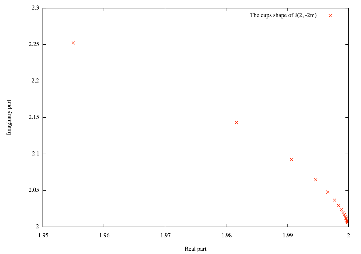
Figure 3. Graph of the cusp shape of $J(2,-2m)$ (from Snappea [Wee99]).

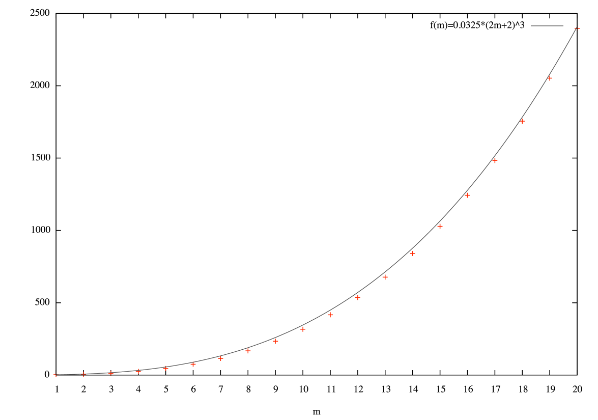
Figure 4. Graph of $|{\mathbb{T}}^{J(2,-2m)}_{\lambda}(\rho_{0})|$ and $f(m)=C(\sharp J(2,-2m))^{3}$.

The graph on Fig. 4 gives the behavior of the sequence of the absolute value of ${\mathbb{T}}^{J(2,-2m)}_{\lambda}(\rho_{0})$ with respect to the number of crossings $\sharp J(2,-2m)=2+2m$ of the knot. The order of growth can be deduced by a “surgery argument”  using Item (5) of Remark 2 and the surgery formula for the Reidemeister torsion [Por97, Theorem 4.1].

Proposition 20.

The sequence $\left({|{\mathbb{T}}^{J(2,-2m)}_{\lambda}(\rho_{0})|}\right)_{m\geqslant 1}$ has the same behavior as the sequence $\left({C(\sharp J(2,-2m))^{3}}\right)_{m\geqslant 1}$, for some constant $C$.

Ideas of the Proof.

Item (5) of Remark 2 gives us that $E_{J(2,-2m)}=\mathcal{W}(1/m)$ is obtained by a surgery of slope $1/m$ on the trivial component of the Whitehead link $\mathcal{W}$. Let $V$ denote the glued solid torus and $\gamma$ its core. Using [Por97, Theorem 4.1 (iii) and Proposition 2.25] we have, up to sign:

(55) $${\mathbb{T}}^{J(2,-2m)}_{\lambda}(\rho_{0})={\mathbb{T}}^{\mathcal{W}}_{(\lambda,\mu^{\prime}{\lambda^{\prime}}^{-m})}(\rho_{0})\cdot\mathrm{TOR}(V;\mathfrak{sl}_{2}({\mathbb{C}})_{\rho_{0}},\gamma)$$

where ${\mathbb{T}}^{\mathcal{W}}_{(\lambda,\mu^{\prime}{\lambda^{\prime}}^{-m})}(\rho_{0})$ stands for the $(Ad\circ\rho_{0})$-non–abelian Reidemeister torsion of the Whitehead link exterior computed with respect to the bases of the twisted homology groups determined by the two curves $\lambda$, and $\mu^{\prime}{\lambda^{\prime}}^{-m}$ (see [Por97, Theorem 4.1]), and $\mathrm{TOR}(V;\mathfrak{sl}_{2}({\mathbb{C}})_{\rho_{0}},\gamma)$ stands for the $(Ad\circ\rho_{0})$-non–abelian Reidemeister torsion of the solid torus $V$ computed with respect to its core $\gamma$. Here $\rho_{0}$ denotes the holonomy representation of the Whitehead link exterior.

To obtain the behavior of ${\mathbb{T}}^{J(2,-2m)}_{\lambda}(\rho_{0})$ we estimate the two terms on the right–hand side of Eq. (55):

1. Using [Por97, Proof of Theorem 4.17], it is easy to see that $\mathrm{TOR}(V;\mathfrak{sl}_{2}({\mathbb{C}})_{\rho_{0}},\gamma)$ goes as $\frac{1}{4\pi^{2}}m^{2}$ when $m$ goes to infinity.

2. Using [Por97, Theorem 4.1 (ii)], one can prove that

   $${\mathbb{T}}^{\mathcal{W}}_{(\lambda,\mu^{\prime}{\lambda^{\prime}}^{-m})}(\rho_{0})={\mathbb{T}}^{\mathcal{W}}_{(\lambda,\lambda^{\prime})}(\rho_{0})\cdot\left(\frac{1}{{\mathfrak{c}}(\lambda,\mu)}-m\right),$$

   where ${\mathfrak{c}}={\mathfrak{c}}(\lambda,\mu)$ denotes the cusp shape of $J(2,-2m)$ (computed with respect to the usual meridian–longitude system). Thus, ${\mathbb{T}}^{\mathcal{W}}_{(\lambda,\mu^{\prime}{\lambda^{\prime}}^{-m})}(\rho_{0})$ goes as ${\mathbb{T}}^{\mathcal{W}}_{(\lambda,\lambda^{\prime})}(\rho_{0})\cdot m$ when $m$ goes to infinity. One can also prove that, at the holonomy, we have

   $${\mathbb{T}}^{\mathcal{W}}_{(\lambda,\lambda^{\prime})}(\rho_{0})=8(1+i).$$

As a result, ${\mathbb{T}}^{J(2,-2m)}_{\lambda}(\rho_{0})$ goes as $C\cdot m^{3}$ for some constant $C$. ∎

Appendix A Program list and Tables

A.1. Program list for Maxima

We give a program list in order to compute the twisted Reidemeister torsion for a given twist knot. This program works on the free computer algebra system Maxima [Sa06]. The function $R(m)$ in the list computes the Riley polynomial of $J(2,2m)$. The function $T(m)$ computes the twisted Reidemeister torsion for $J(2,2m)$. It gives a polynomial of $s$ and $u$ such that the top degree of $u$ is lower than that in the Riley polynomial $\phi_{J(2,2m)}(s,u)$. Here we use Expressions (49) & (51) and the following remark for computing the twisted Reidemeister torsion.

Remark 24.

It follows from Equation $(\ref{eqn:Riley_poly})$ that the highest degree term of $u$ in $\phi_{J(2,2m)}(s,u)$ is equal to $-u^{2m-1}$ (resp. $u^{2|m|}$) if $m>0$ (resp. $m<0$).

Program list

load("nchrpl");/*We need this package for using mattrace*/
R(m):=block(/*function for calculating the Riley polynomial of J(2,2m)*/
        [/*w is the matrix of w=[y,x^{-1}]*/
         w:matrix([1-s*u,1/s-u-1],[-u+s*u*(u+1),(-u)/s+(u+1)^2]),
         p],
        w:w^^m,
        p:w[1,1]+(1-s)*w[1,2],
        p:expand(p),
        return(p)
      );
T(m):=if integerp(m) then
        if m=0 then "J(2,0) is unknot." else
          block(
            [/*matrix for adjoint action of x*/
             X:matrix([s,-2,(-1)/s],[0,1,1/s],[0,0,1/s]),
             /*matrix for adjoint action of y*/
             Y:matrix([s,0,0],[s*u,1,0],[(-s)*u^2,(-2)*u,1/s]),
             IX,/*inverse matrix of X*/
             IY,/*inverse matrix of Y*/
             S:ident(3),/*marix for series of W or W^{-1}*/
             AS:ident(3),/*adjoint matrix of S*/
             W,/*matrix W=[Y,IX] */
             IW,/*matrix [IX,Y]*/
             d:1,/*the highest degree of u in the numerator
                    of R-torsion*/
             k:1,/*the highest degree of u in the Riley poly*/
             p:0,
             r:R(m),/*the Riley poly*/
             r1 /*a polynomial removed the top term of u
                  from the Riley polynomial*/
            ],
            IX:invert(X),
            IY:invert(Y),
            W:Y.IX.IY.X,
            IW:IX.Y.X.IY,
            /*calculating the numerator of R-torsion*/
            if m>0 then
              block(
                /*calculation of S*/
                for i:1 thru m-1 do(S:ident(3)+S.IW),
                AS:adjoint(S),
                /*the numerator of R-torsion*/
                p:p+mattrace(IX.S),
                p:p+3*mattrace(X.AS)+mattrace(IY.W.AS),
                p:p-mattrace(IX.S)*mattrace((ident(3)+IX.Y).S),
                p:p+mattrace(IX.S.(ident(3)+IX.Y).S),
                p:p+(2-s+(-1)/s)^2*determinant(S),
                /*The top term of u in the Riley poly r
                   is given by -u^(2m-1).
                  We use the relation u^(2m-1) = r + u^(2m-1) later*/
                k:2*m-1,/*the highets degree of u in the Riley poly*/
                r1:r+u^(2*m-1)
              )
            else
              block(
                /*calculation of S*/
                for i:1 thru -m-1 do(S:ident(3)+S.W),
                AS:adjoint(S),
                p:p-mattrace(IX.S.W),
                p:p+3*mattrace(X.IW.AS)+mattrace(IY.AS),
                p:p-mattrace(IX.S.W)*mattrace((ident(3)+IX.Y).S.W),
                p:p+mattrace(IX.S.W.(ident(3)+IX.Y).S.W),
                p:p-(2-s+(-1)/s)^2*determinant(S),
                /*The top term of u in the Riley poly r
                   is given by u^(2|m|).
                  We use the relation u^(2|m|) = -r + u^(2|m|) later*/
                k:2*(-m),/*the highets degree of u in the Riley poly*/
                r1:-r+u^(2*(-m))
              ),
            p:expand(p),
            /* simplify by using r (decreasing the degrees of u)*/
            /* set the degree of u in p*/
            d:hipow(p,u),
            /*decreasing the degrees of u*/
            for j:1 while d >= k do(
              p:subst(r1*u^(d-k),u^d,p),
              p:expand(p),
              d:hipow(p,u)
            ),
            p:factor(p),
            /*multiplying p
               by the denominator of twisted Alexander*/
            p:expand(p*(s/(s^2-2*s+1))),
            p:factorout(p,s),
            r:factorout(r,s),
            print("The Riley polynomial of J(2,",2*m,"):",r),
            print("The Reidemeister torsion for J(2,",2*m,"):"),
            return(p)
          )
      else print(m,"is not an integer.");

A.2. Tables

In this appendix, except in the case of the trefoil knot (the only twist knot which is not hyperbolic), $u$ denotes the root of Riley’s equation $\phi_{K}(1,u)=0$ corresponding to the discrete and faithful representation of the complete hyperbolic structure.

Tables 1 and 2 give the non–abelian Reidemeister torsion for twist knots at the holonomy (except in the case of the trefoil) with respect to the corresponding root of Riley’s equation and to the cusp shape of the knot exterior.

Non–abelian torsion for $J(2,2m)$  $(1\leq m\leq 10)$
$m$	Torsion at the holonomy ${\mathbb{T}}^{J(2,2m)}_{\lambda}(\rho_{u})$ (divided by a sign $-\tau_{0}$)
	Result by substituting $u=4/({\mathfrak{c}}-2)$ into ${\mathbb{T}}^{J(2,2m)}_{\lambda}(\rho_{u})$, where ${\mathfrak{c}}$ is the cusp shape
$1$	$3$
	$3$
$2$	$13u^{2}-7u+19$
	$(19{\mathfrak{c}}^{2}-104{\mathfrak{c}}+340)/({\mathfrak{c}}-2)^{2}$
$3$	$26u^{4}-17u^{3}+98u^{2}-45u+55$
	$(55{\mathfrak{c}}^{4}-620{\mathfrak{c}}^{3}+3968{\mathfrak{c}}^{2}-11280{\mathfrak{c}}+17424)/({\mathfrak{c}}-2)^{4}$
$4$	$46u^{6}-34u^{5}+263u^{4}-157u^{3}+402u^{2}-159u+118$
	$2(59{\mathfrak{c}}^{6}-1026{\mathfrak{c}}^{5}+9936{\mathfrak{c}}^{4}-52912{\mathfrak{c}}^{3}+180592{\mathfrak{c}}^{2}-352032{\mathfrak{c}}+369280)/({\mathfrak{c}}-2)^{6}$
$5$	$69u^{8}-54u^{7}+540u^{6}-366u^{5}+1360u^{4}-733u^{3}+1186u^{2}-411u+215$
	$(215{\mathfrak{c}}^{8}-5084{\mathfrak{c}}^{7}+66072{\mathfrak{c}}^{6}-509040{\mathfrak{c}}^{5}+2656960{\mathfrak{c}}^{4}-9378624{\mathfrak{c}}^{3}+22613632{\mathfrak{c}}^{2}-33723648{\mathfrak{c}}+26688768)/({\mathfrak{c}}-2)^{8}$
$6$	$99u^{10}-81u^{9}+971u^{8}-710u^{7}+3400u^{6}-2123u^{5}+5052u^{4}-2469u^{3}+2875u^{2}-884u+353$
	$(353{\mathfrak{c}}^{10}-10596{\mathfrak{c}}^{9}+173188{\mathfrak{c}}^{8}-1742080{\mathfrak{c}}^{7}+12219808{\mathfrak{c}}^{6}-61550208{\mathfrak{c}}^{5}+228030592{\mathfrak{c}}^{4}-612284416{\mathfrak{c}}^{3}+1160955136{\mathfrak{c}}^{2}-1411093504{\mathfrak{c}}+903214080)/({\mathfrak{c}}-2)^{10}$
$7$	$132u^{12}-111u^{11}+1566u^{10}-1203u^{9}+7057u^{8}-4810u^{7}+14996u^{6}-8647u^{5}+15044u^{4}-6710u^{3}+6076u^{2}-1678u+539$
	$(539{\mathfrak{c}}^{12}-19648{\mathfrak{c}}^{11}+387176{\mathfrak{c}}^{10}-4799040{\mathfrak{c}}^{9}+42208784{\mathfrak{c}}^{8}-274741248{\mathfrak{c}}^{7}+1363062528{\mathfrak{c}}^{6}-5187840000{\mathfrak{c}}^{5}+15118560512{\mathfrak{c}}^{4}-33001455616{\mathfrak{c}}^{3}+51856091136{\mathfrak{c}}^{2}-53202206720{\mathfrak{c}}+28544299008)/({\mathfrak{c}}-2)^{12}$
$8$	$172u^{14}-148u^{13}+2383u^{12}-1899u^{11}+13098u^{10}-9475u^{9}+36258u^{8}-23106u^{7}+52884u^{6}-28275u^{5}+38518u^{4}-15774u^{3}+11636u^{2}-2914u+780$
	$4(195{\mathfrak{c}}^{14}-8374{\mathfrak{c}}^{13}+193288{\mathfrak{c}}^{12}-2846448{\mathfrak{c}}^{11}+30095568{\mathfrak{c}}^{10}-239812000{\mathfrak{c}}^{9}+1487434752{\mathfrak{c}}^{8}-7287857664{\mathfrak{c}}^{7}+28404952320{\mathfrak{c}}^{6}-87772645888{\mathfrak{c}}^{5}+212579837952{\mathfrak{c}}^{4}-393068802048{\mathfrak{c}}^{3}+529782681600{\mathfrak{c}}^{2}-471281852416{\mathfrak{c}}+218188021760)/({\mathfrak{c}}-2)^{14}$
$9$	$215u^{16}-188u^{15}+3416u^{14}-2796u^{13}+22210u^{12}-16767u^{11}+76022u^{10}-51847u^{9}+146639u^{8}-87602u^{7}+157972u^{6}-78647u^{5}+87864u^{4}-33238u^{3}+20652u^{2}-4730u+1083$
	$(1083{\mathfrak{c}}^{16}-53576{\mathfrak{c}}^{15}+1417872{\mathfrak{c}}^{14}-24177568{\mathfrak{c}}^{13}+298484224{\mathfrak{c}}^{12}-2810875520{\mathfrak{c}}^{11}+20889506048{\mathfrak{c}}^{10}-124832580096{\mathfrak{c}}^{9}+606632721920{\mathfrak{c}}^{8}-2406783375360{\mathfrak{c}}^{7}+7784342106112{\mathfrak{c}}^{6}-20354210914304{\mathfrak{c}}^{5}+42341634637824{\mathfrak{c}}^{4}-68068269064192{\mathfrak{c}}^{3}+80435317243904{\mathfrak{c}}^{2}-63142437978112{\mathfrak{c}}+25688198283264)/({\mathfrak{c}}-2)^{16}$
$10$	$265u^{18}-235u^{17}+4739u^{16}-3964u^{15}+35520u^{14}-27711u^{13}+144776u^{12}-103759u^{11}+348155u^{10}-224404u^{9}+501055u^{8}-281458u^{7}+417368u^{6}-194245u^{5}+183500u^{4}-64454u^{3}+34537u^{2}-7285u+1455$
	$(1455{\mathfrak{c}}^{18}-81520{\mathfrak{c}}^{17}+2433812{\mathfrak{c}}^{16}-47158400{\mathfrak{c}}^{15}+665730240{\mathfrak{c}}^{14}-7230947840{\mathfrak{c}}^{13}+62585931008{\mathfrak{c}}^{12}-440831379456{\mathfrak{c}}^{11}+2561522930176{\mathfrak{c}}^{10}-12371911213056{\mathfrak{c}}^{9}+49827680770048{\mathfrak{c}}^{8}-167134091640832{\mathfrak{c}}^{7}+464297966682112{\mathfrak{c}}^{6}-1056316689612800{\mathfrak{c}}^{5}+1931794260754432{\mathfrak{c}}^{4}-2753296051208192{\mathfrak{c}}^{3}+2901909811167232{\mathfrak{c}}^{2}-2040504620417024{\mathfrak{c}}+741196988416000)/({\mathfrak{c}}-2)^{18}$

Table 1. Table for the sequence of knots $J(2,2m)$, $(1\leq m\leq 10)$.

Non–abelian torsion for $J(2,-2m)$  $(1\leq m\leq 10)$
$m$	Torsion at the holonomy ${\mathbb{T}}^{J(2,-2m)}_{\lambda}(\rho_{u})$ (divided by a sign $\tau_{0}$)
	Result by substituting $u=4/({\mathfrak{c}}-2)$ into ${\mathbb{T}}^{J(2,-2m)}_{\lambda}(\rho_{u})$, where ${\mathfrak{c}}$ is the cusp shape
$1$	$-3$
	$-3$
$2$	$7u^{3}+u^{2}+14u-5$
	$-(5{\mathfrak{c}}^{3}-86{\mathfrak{c}}^{2}+268{\mathfrak{c}}-680)/({\mathfrak{c}}-2)^{3}$
$3$	$17u^{5}+8u^{4}+79u^{3}+26u^{2}+73u+1$
	$({\mathfrak{c}}^{5}+282{\mathfrak{c}}^{4}-1880{\mathfrak{c}}^{3}+9488{\mathfrak{c}}^{2}-22448{\mathfrak{c}}+34848)/({\mathfrak{c}}-2)^{5}$
$4$	$34u^{7}+22u^{6}+225u^{5}+119u^{4}+439u^{3}+162u^{2}+229u+22$
	$2(11{\mathfrak{c}}^{7}+304{\mathfrak{c}}^{6}-3276{\mathfrak{c}}^{5}+25488{\mathfrak{c}}^{4}-112432{\mathfrak{c}}^{3}+359808{\mathfrak{c}}^{2}-661824{\mathfrak{c}}+738560)/({\mathfrak{c}}-2)^{7}$
$5$	$54u^{9}+39u^{8}+474u^{7}+300u^{6}+1411u^{5}+730u^{4}+1619u^{3}+586u^{2}+551u+65$
	$(65{\mathfrak{c}}^{9}+1034{\mathfrak{c}}^{8}-16528{\mathfrak{c}}^{7}+175520{\mathfrak{c}}^{6}-1125280{\mathfrak{c}}^{5}+5374144{\mathfrak{c}}^{4}-17783040{\mathfrak{c}}^{3}+42336768{\mathfrak{c}}^{2}-62848768{\mathfrak{c}}+53377536)/({\mathfrak{c}}-2)^{9}$
$6$	$81u^{11}+63u^{10}+872u^{9}+611u^{8}+3462u^{7}+2104u^{6}+6167u^{5}+3036u^{4}+4714u^{3}+1615u^{2}+1129u+137$
	$(137{\mathfrak{c}}^{11}+1502{\mathfrak{c}}^{10}-34340{\mathfrak{c}}^{9}+468616{\mathfrak{c}}^{8}-3940960{\mathfrak{c}}^{7}+25007808{\mathfrak{c}}^{6}-117308544{\mathfrak{c}}^{5}+420442368{\mathfrak{c}}^{4}-1109472000{\mathfrak{c}}^{3}+2123257344{\mathfrak{c}}^{2}-2628703232{\mathfrak{c}}+1806428160)/({\mathfrak{c}}-2)^{11}$
$7$	$111u^{13}+90u^{12}+1425u^{11}+1062u^{10}+7105u^{9}+4747u^{8}+17286u^{7}+9956u^{6}+21045u^{5}+9752u^{4}+11610u^{3}+3724u^{2}+2070u+245$
	$(245{\mathfrak{c}}^{13}+1910{\mathfrak{c}}^{12}-62696{\mathfrak{c}}^{11}+1057552{\mathfrak{c}}^{10}-11025808{\mathfrak{c}}^{9}+87196704{\mathfrak{c}}^{8}-526180096{\mathfrak{c}}^{7}+2499806720{\mathfrak{c}}^{6}-9272200448{\mathfrak{c}}^{5}+26825366016{\mathfrak{c}}^{4}-58773907456{\mathfrak{c}}^{3}+94191718400{\mathfrak{c}}^{2}-99494326272{\mathfrak{c}}+57088598016)/({\mathfrak{c}}-2)^{13}$
$8$	$148u^{15}+124u^{14}+2195u^{13}+1711u^{12}+13125u^{11}+9354u^{10}+40453u^{9}+25698u^{8}+68070u^{7}+37044u^{6}+60745u^{5}+26422u^{4}+25394u^{3}+7604u^{2}+3502u+396$
	$4(99{\mathfrak{c}}^{15}+532{\mathfrak{c}}^{14}-26060{\mathfrak{c}}^{13}+529856{\mathfrak{c}}^{12}-6606160{\mathfrak{c}}^{11}+62595520{\mathfrak{c}}^{10}-460836032{\mathfrak{c}}^{9}+2719805952{\mathfrak{c}}^{8}-12910096128{\mathfrak{c}}^{7}+49528327168{\mathfrak{c}}^{6}-152285103104{\mathfrak{c}}^{5}+370984124416{\mathfrak{c}}^{4}-695663718400{\mathfrak{c}}^{3}+961422573568{\mathfrak{c}}^{2}-884915453952{\mathfrak{c}}+436376043520)/({\mathfrak{c}}-2)^{15}$
$9$	$188u^{17}+161u^{16}+3172u^{15}+2552u^{14}+22171u^{13}+16540u^{12}+82961u^{11}+56366u^{10}+179181u^{9}+108029u^{8}+224190u^{7}+115204u^{6}+154037u^{5}+62916u^{4}+50650u^{3}+14172u^{2}+5570u+597$
	$(597{\mathfrak{c}}^{17}+1982{\mathfrak{c}}^{16}-161440{\mathfrak{c}}^{15}+3885760{\mathfrak{c}}^{14}-56503104{\mathfrak{c}}^{13}+624108160{\mathfrak{c}}^{12}-5417133568{\mathfrak{c}}^{11}+38142084096{\mathfrak{c}}^{10}-219869856256{\mathfrak{c}}^{9}+1045959103488{\mathfrak{c}}^{8}-4105465389056{\mathfrak{c}}^{7}+13257704030208{\mathfrak{c}}^{6}-34864687169536{\mathfrak{c}}^{5}+73473552449536{\mathfrak{c}}^{4}-120432383098880{\mathfrak{c}}^{3}+146315203575808{\mathfrak{c}}^{2}-119078046597120{\mathfrak{c}}+51376396566528)/({\mathfrak{c}}-2)^{17}$
$10$	$235u^{19}+205u^{18}+4434u^{17}+3659u^{16}+35404u^{15}+27360u^{14}+155687u^{13}+111176u^{12}+410964u^{11}+266255u^{10}+665399u^{9}+380935u^{8}+647346u^{7}+314408u^{6}+353985u^{5}+135980u^{4}+94041u^{3}+24637u^{2}+8440u+855$
	$(855{\mathfrak{c}}^{19}+1270{\mathfrak{c}}^{18}-236348{\mathfrak{c}}^{17}+6649256{\mathfrak{c}}^{16}-110706240{\mathfrak{c}}^{15}+1397436800{\mathfrak{c}}^{14}-13965196032{\mathfrak{c}}^{13}+114155938304{\mathfrak{c}}^{12}-773068443136{\mathfrak{c}}^{11}+4380077954048{\mathfrak{c}}^{10}-20842143467520{\mathfrak{c}}^{9}+83401615028224{\mathfrak{c}}^{8}-279834167951360{\mathfrak{c}}^{7}+782314999349248{\mathfrak{c}}^{6}-1800640172326912{\mathfrak{c}}^{5}+3349441682210816{\mathfrak{c}}^{4}-4881403696185344{\mathfrak{c}}^{3}+5296224268058624{\mathfrak{c}}^{2}-3862939033141248{\mathfrak{c}}+1482393976832000)/({\mathfrak{c}}-2)^{19}$

Table 2. Table for the sequence of knots $J(2,-2m)$, $(1\leq m\leq 10)$.

References

• [Ada94] C. Adams, The knot book, W. H. Freeman and Company, 1994.
• [Cal06] D. Calegari, Real places and torus bundles, Geom. Dedicata 118 (2006), 209–227.
• [CGLS87] M. Culler, C. McA. Gordon, J. Luecke, and P. Shalen, Dehn surgery on knots, Ann. of Math. 125 (1987), 237–300.
• [CS83] M. Culler and P. Shalen, Varieties of group representations and splittings of $3$-manifolds, Ann. of Math. 117 (1983), 109–146.
• [DK07] J. Dubois and R. Kashaev, On the asymptotic expansion of the colored Jones polynomial for torus knots, Math. Ann. 339 (2007), 757–782.
• [Dub05] J. Dubois, Non abelian Reidemeister torsion and volume form on the ${\mathrm{SU}}(2)$-representation space of knot groups, Ann. Institut Fourier 55 (2005), 1685–1734.
• [Dub06] by same author, Non abelian twisted Reidemeister torsion for fibered knots, Canad. Math. Bull. 49 (2006), 55–71.
• [FV07] S. Friedl and S. Vidussi, Symplectic $\text{S}^{1}\times{N}^{3}$, subgroup separability, and vanishing Thurston norm, 2007, preprint arXiv:math/0701717.
• [GKM05] H. Goda, T. Kitano, and T. Morifuji, Reidemeister torsion, twisted Alexander polynomial and fibered knots, Comment. Math. Helv. 80 (2005), 51–61.
• [Heu03] M. Heusener, An orientation for the $\mathrm{SU}(2)$-representation space of knot groups, Topology and its Applications 127 (2003), 175–197.
• [HS04] J. Hoste and P. D. Shanahan, A formula for the A-polynomial of twist knots, J. Knot Theory Ramifications 13 (2004), 193–209.
• [Kit96] T. Kitano, Twisted Alexander polynomial and Reidemeister torsion, Pacific J. Math. 174 (1996), 431–442.
• [KL99] P. Kirk and C. Livingston, Twisted Alexander Invariants, Reidemeister torsion, and Casson-Gordon invariants, Topology 38 (1999), 635–661.
• [Le94] T. Le, Varieties of representations and their subvarieties of cohomology jumps for certain knot groups, Russian Acad. Sci. Sb. Math. 78 (1994), 187–209.
• [Lei02] C. J. Leininger, Surgeries on one component of the Whitehead link are virtually fibered, Topology 41 (2002), 307–320.
• [Lin01] X-S. Lin, Representations of knot groups and twisted Alexander polynomials, Acta Math. Sin. (Engl. Ser.) 17 (2001), no. 3, 361–380.
• [Men84] W. Menasco, Closed incompressible surfaces in alternating knot and link complements, Topology 23 (1984), 37–44.
• [Mer03] R. Merris, Combinatorics, 2nd ed., John Wiley and Sons, 2003.
• [Mil66] J. Milnor, Whitehead torsion, Bull. Amer. Math. Soc. 72 (1966), 358–426.
• [Por97] J. Porti, Torsion de Reidemeister pour les variétés hyperboliques, vol. 128, Mem. Amer. Math. Soc., no. 612, AMS, 1997.
• [Ril84] R. Riley, Nonabelian representations of $2$-bridge knot groups, Quart. J. Math. Oxford Ser. $(2)$ 35 (1984), 191–208.
• [Rol90] D. Rolfsen, Knots and links, Publish or Perish Inc., 1990.
• [Sa06] W. Schelter and al, Maxima, 2006, available at http://maxima.sourceforge.net/.
• [Sha02] P. B. Shalen, Representations of $3$-manifold groups, Handbook of Geometric Topology (R. J. Daverman and R. B. Sher, eds.), North-Holland Amsterdam, 2002, pp. 955–1044.
• [SW06] D. Silver and S. Williams, Twisted Alexander polynomials detect the unknot, Algebr. Geom. Topol. 6 (2006), 1903–1923.
• [Thu02] W. Thurston, The Geometry and Topology of Three-Manifolds, Electronic Notes available at http://www.msri.org/publications/books/gt3m/, 2002.
• [Tur01] V. Turaev, Introduction to combinatorial torsions, Lectures in Mathematics, Birkhäuser, 2001.
• [Tur02] by same author, Torsions of $3$-dimensional manifolds, Progress in Mathematics, vol. 208, Birkhäuser, 2002.
• [Wad94] M. Wada, Twisted Alexander polynomial for finitely presentable groups, Topology 33 (1994), no. 2, 241–256.
• [Wal78] F. Waldhausen, Algebraic K-theory of generalized free products I, II., Ann. of Math. 108 (1978), 135–204.
• [Wee99] J. Weeks, SnapPea, 1999, available at http://www.geometrygames.org/SnapPea/.
• [Yam05] Y. Yamaguchi, A relationship between the non-acyclic Reidemeister torsion and a zero of the acyclic Reidemeister torsion, 2005, to appear in Ann. Institut Fourier (arXiv:math.GT/0512267).
• [Yam07] Y. Yamaguchi, Limit values of the non-acyclic Reidemeister torsion for knots, Algebr. Geom. Topol. 7 (2007), 1485–1507.