Nanorheology of viscoelastic shells: Applications to viral capsids

Abstract

We study the microrheology of nanoparticle shells [Dinsmore et al. Science 298, 1006 (2002)] and viral capsids [Ivanovska et al. PNAS 101, 7600 (2004)] by computing the mechanical response function and thermal fluctuation spectrum of a viscoelastic spherical shell that is permeable to the surrounding solvent. We determine analytically the damped dynamics of the shear, bend, and compression modes of the shell coupled to the solvent both inside and outside the sphere in the zero Reynolds number limit. We identify fundamental length and time scales in the system, and compute the thermal correlation function of displacements of antipodal points on the sphere and the mechanical response to pinching forces applied at these points. We describe how such a frequency-dependent antipodal correlation and/or response function, which should be measurable in new AFM-based microrheology experiments, can probe the viscoelasticity of these synthetic and biological shells constructed of nanoparticles.

I Introduction

Understanding the dynamics of soft, nanoporous materials will be an important area of research both in biophysics and in the materials science communities. This emerging field of study is being driven by new AFM-based mechanical or rheological measurements of supramolecular biological materials Dufrene:03 ; Radhakrishnan:04 and even entire cells You:99 ; Alonso:02 . Perhaps the prototypical examples of such a material are found in the plethora of viral capsids. Such shells are constructed from a small set of proteins or their oligomers (capsomeres) arranged in an ordered structure forming roughly a spherical shell. The packing of these capsomeres generically leaves at least nanometer scale pores through which solvent may flow. In addition, there is a wide variety of similarly nanoporous synthetic structures such as linked networks of nanoparticles Lin:03 and colloids Dinsmore:02 ; Lawrence:07 assembled into two-dimensional shells. In both the biological and synthetic cases, the material making up the thin shell or membrane is constructed from identical nanoscale tiles that incorporate holes of comparable size through which the solvent may flow. Other examples of porous membranes include lipid bilayers containing pore-forming transmembrane proteins Gilbert:02 ; Janshoff:06 and even the large ($\sim 100$nm) cytoplasmic ribonucleoprotein vaults Kedersha:86 , which make up a rather ubiquitous but enigmatic component of eukaryotic cells.

We focus on elucidating the mechanical response of such a permeable shell to a set of sinusoidally time-varying “pinching” forces applied at antipodal points on the sphere – see Fig. 1(a). Such forces represent the simplest characterization of an AFM-based nanoindentation experiment performed at finite frequency. By applying known forces at a fixed frequency and observing the in-phase and out-of-phase response of the diameter $D$ of the spherical shell one should be able to extract the viscoelastic properties of the shell material. Such an experiment is the finite-frequency generalization of the work of Michel et al. Michel:06 and can be considered to be an active microrheological measurement. Alternatively, one may imagine that the AFM tip can be used in a passive manner to monitor the thermal fluctuations of this diameter. Since a number of these physically relevant shells are rather incompliant, their thermal fluctuations are likely to be unresolvable. In such cases passive microrheology (i.e. the monitoring of thermally fluctuating variables) must be supplanted by active techniques. This distinction is of little importance for our analysis provided that the mechanical perturbation in the active technique is small enough that the system remains in its linear response regime. In the passive technique one has direct access to the power spectrum of the fluctuating quantity determined (via the fluctuation dissipation theorem) by the imaginary part of the response function. The real part is then obtained by a Kramers-Krönig relation Landau:51 . In the active measurement the real and imaginary parts of the response function are found directly from the in-phase and out-of-phase response of the shell respectively. In this article we will compute the full frequency-dependent, complex response function as well as the expected thermal power spectrum of $\langle|D(\omega)|^{2}\rangle$ of each shell studied.

To understand the mechanics/dynamics of such nanoscale objects in solution, one must consider the coupled dynamics of soft membranes/shells and the surrounding solvent. The case of viscous shells that are impermeable to the surrounding solvent has been well-studied in the context of microemulsions and vesicles Milner:87 . The focus of our current study, however, is the dynamics of membranes or shells that are permeable to the surrounding solvent on time-scales relevant to the experiment. The effect of solvent permeation, which we quantify below, is to create a new dissipative stress on the shell related to solvent permeation.

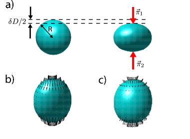
Figure 1: (color online) a) A schematic illustration of an AFM-based rheological experiment on a nanoscale shell. The (red) arrows depict the applied stresses $\bm{\pi}_{1}=-\bm{\pi}_{2}$ that deform the (blue) shell of radius $R$ from a sphere on the left into an oblate object shown in the right. The total change in sphere’s diameter along the line of force application is $\delta D$. This deformation can be resolved into a linear superposition of two sets of normal modes. In b) we show the Lennon-Brochard $\ell=2$ mode while in c) we show the compression dominated longitudinal sound $\ell=2$ mode. In each figure the (black) arrows represent the velocity field of the sphere.

These dissipative (out-of-phase) stresses associated with fluid permeation must also be taken into account for the quantitatively correct interpretation of such measurements as described above. In particular in the case of a membrane or shell that has an inherent viscoelastic response, one may ask whether it remains possible to distinguish the dissipative stresses due to from the material from those associated with fluid permeation.

In this article we quantify and explore the effects of membrane permeability on the dynamics of both flat and spherical membranes. We parameterize the continuum mechanics of the shells by a permeation coefficient, a bending modulus, an area compression modulus, and a two-dimensional, in-plane shear modulus. These latter two moduli we will allow to be viscoelastic, i.e. complex and frequency dependent. We discuss the interpretation of this generalization below. We show that solvent permeability leads to a new dissipative stress in the system that changes the relaxation rates of each deformation mode of the system. We show also that, on a spherical shell, these normal modes are superpositions of compression and bending deformations. We then consider four test cases to explore the interrelated roles of shell porosity and viscoelasticity in determining their mechanical response.

First, we examine the expected response of a purely elastic, porous shell to isolate the dissipative effects of the interaction of the porous shell with the surrounding solvent. We then consider the case of a highly incompressible, but purely viscous membrane of varying porosity. Such systems are reminiscent of giant unilamellar vesicles (GUVs) Dietrich:01 ; Veatch:02 ; Veatch:03 containing pore-forming proteins Ojcius:91 ; Abrami:98 ; Kaneko:04 .

Finally, we consider two simple models of a viscoelastic shell inspired by viral capsids. In the first case we assume that the shell has a purely elastic response to compression but a viscoelastic response to in-plane shear stresses. Such a viscoelastic response to in-plane shear may result from plastic rearrangements of capsomere proteins under applied stresses. Thus, the proteinaceous shell of a virus may deform like an amorphous solid. In the second case we assume an elastic response to in-plane shear stress, but the dissipative relaxation of in-plane compressional stress. Such stress relaxation should occur in cases where the capsomeres have internal degrees of freedom associated with allosteric conformational transitions Conway:95 ; Steven:05 ; Guerin:07 that change their cross-sectional area or packing density. To model this effect we assume a compressional stress relaxation time on a scale typical of known allosteric transitions in proteins. In both cases we employ the simplest model of viscoelasticity, the Maxwell model Bird:77 , which has a single stress-relaxation time scale.

The central question we address is whether it is possible to extract the dissipative mechanics of the capsid proteins from the proposed AFM-based microrheological experiment. It is possible that the dissipative stresses associated with internal rearrangements of the capsomeres or plastic deformations of the shell will be lost against the background of dissipative forces associated with solvent flow through the porous membrane. In both cases, owing to a separation of time scales, the nanoindentation experiment should be able to resolve the expected viscoelastic response of the shell. We show, however, that in the former case of a viscoelastic shear response, the mechanical signature is quite subtle in the real part of the response function due to the dominance of the bending and compression moduli in the response function. However, the imaginary or out-of-phase part of the response function is capable of recording this effect. In the latter case the effect of compressional stress relaxation on time scales typical of protein conformational change should give a dramatic mechanical signature in the imaginary part of the response function so that finite-frequency nanoindentation studies should be an excellent probe of these complex mechanics.

The remainder of the paper is organized as follows. In section II.1 we calculate the effect of porosity on the undulation dynamics of a flat membrane in a viscous solvent. We also discuss expected values of the permeation coefficient for a variety of physically important systems. The calculation of these coefficients is discussed in appendix A. In section II.2 we consider the deformations of a spherical membrane where the curvature of the undeformed structure couples the previously studied bending mode to in-plane compression. To incorporate the mechanical effects of solvent hydrodynamics in the case of spherical shells, we recount and apply the pioneering work of Lamb Lamb:32 and Brenner Brenner:64 on low-Reynolds number flows inside and outside a sphere in section II.3. Using the results of the previous calculations we plot and discuss the decay rates of the linearly independent modes of the shell in section II.4. In section III we use the dynamics of these linearly-independent modes to construct the complex, frequency-dependent response function of the shell to antipodal pinching forces. In sections III.1, III.2, and III.3 we plot the response functions and predicted thermal power spectra of elastic, viscous, and the two classes of viscoelastic shells introduced above. Finally, in section IV, we compare these results and discuss the implications of our work for future nanoindentation-based rheology measurements.

II Calculation

II.1 The plane permeable membrane

The overarching feature of these systems is that fluid flow through the shell or membrane (permeation) can occur on timescales comparable to the relaxation of surface deformations. Thus, the velocity of the fluid at the membrane surface in the direction along the local normal of that surface will not be equal to the normal velocity of the membrane. In the limit of high membrane porosity, the fluid will essentially pass though the membrane undisturbed. Consequently the hydrodynamic interaction of the membrane with itself, which is known to qualitatively alter the spectrum of the decay rates of membrane undulations Brochard:75 is suppressed and replaced by dynamics consistent with local drag. As the porosity or permeability of the membrane is reduced, the system continuously recovers these well-known hydrodynamic self-interactions that control the structure of the spectrum of undulatory decay rates. To better understand this feature we address the dynamics of a plane porous elastic membrane in a viscous Newtonian solvent. We assume that the dynamics are all occurring at low Reynolds number. For a flat membrane or interface the normal modes of the coupled interface and solvent system involve bending in-plane shear and compression Levine:02 . Since we will concentrate on indentation-based measurements, we consider only the undulation mode of the flat membrane.

A zero-tension membrane is characterized by a single bending modulus $\kappa$ so that free energy of the membrane may be written as

$${\cal F}=\frac{\kappa}{2}\int\left[\nabla_{\perp}^{2}w\right]^{2}dxdy,$$ (1)

in terms of normal displacement $w$. Here $\nabla_{\perp}$ is the in-plane gradient operator acting on membrane coordinates $x,y$. In the above we implicitly assumed small deformations of the surface from its flat equilibrium shape. The restoring stresses acting on the deformed membrane are given by

$$f=-\frac{\delta{\cal F}}{\delta w}=-\kappa\nabla_{\perp}^{4}w.$$ (2)

The equation of motion for the fluid of viscosity $\eta$ in the limit of vanishing Reynolds number is the linearized Navier-Stokes equation for an incompressible fluid:

$$\bm{\nabla}\cdot{\bf v}=0$$ (3)

$$\displaystyle\rho\frac{\partial{\bf v}}{\partial t}=\eta\nabla^{2}{\bf v}-\bm{\nabla}p,$$ (4)

where $p$ is the pressure. The interaction between the fluid and the membrane is governed by three boundary conditions enforced at the membrane lying in the $xy$ plane. First, we require Darcy’s law to be obeyed so that the flux of the fluid through a unit area of the membrane is proportional to the pressure difference between the two sides Batchelor:67 . Thus

$$\alpha\left(v_{z}\Big{|}_{z=0}-\frac{dw}{dt}\right)=p^{-}-p^{+},$$ (5)

where $p^{+,-}$ are the pressures above ($z>0$) and below ($z<0$) the membrane respectively. We discuss the estimation of the Darcy coefficient $\alpha$ in terms of the microscale structure of the membrane in Appendix A. Expected values of the permeation coefficient for a variety of systems are given in Table 1. This first boundary condition relates the normal velocities of the membrane and fluid at the membrane surface by equating the normal stress difference across the membrane to the fluid flow through it. In addition we must insist upon the continuity of the normal component of the fluid velocity so that

$$v_{z}^{+}(0)=v_{z}^{-}(0),$$ (6)

where $v_{z}^{\pm}(0)=\lim_{z\to 0^{\pm}}v_{z}(z)$. For the tangential velocities, we enforce a no-slip boundary condition on the fluid at the upper and lower boundaries of the membrane:

$$v_{x}^{+}(0)=v_{x}^{-}(0)=0.$$ (7)

Finally, we require the fluid velocity field and pressure to vanish infinitely far from the membrane so that

$${\bf v}(\pm\infty)=0,\quad p(\pm\infty)=0.$$ (8)

Ignoring the inertia of the membrane, we require force balance between the elastic restoring stress $f$ from Eq. (2), the viscous stresses $\sigma^{+}_{zz}$ and $\sigma^{-}_{zz}$ exerted by the fluid on both sides of the membrane and an externally imposed stress, $\pi_{e}$ so that

$$(\sigma_{zz}^{-}-\sigma_{zz}^{+})\Bigl{|}_{z=0}+\,\pi_{e}=\kappa\bm{\nabla}^{4}w.$$ (9)

Table 1: Dimensionless permeation coefficients (Eq. (79)) for nanoscale capsules

System	Permeation coefficient	Ref
Rotavirus	50	Johnson:97
S-layer shell	$10^{4}$	S-layer:97
Colloidosome	$10^{4}-10^{5}$	Dinsmore:02
GUV	$10-\infty$	Gilbert:02 ; Janshoff:06

To compute the decay rate of membrane undulations having wave vector $q$, we consider a sinusoidally applied normal stress $\pi_{e}$

$$\pi_{e}=\pi\,e^{iqx-i\omega t},$$ (10)

and look for solutions of the membrane deformation taking form of

$$w=w_{0}e^{iqx-i\omega t}.$$ (11)

Details of the calculation are presented in Appendix B. In the limit that viscous stresses dominate inertial ones in the fluid, i.e. $\omega\rho\ll\eta q^{2}$, we find that the amplitude of the driven undulations is given by

$$w_{0}=-\frac{\pi\,\left[\frac{\alpha}{2\,q\,\eta}+2\right]}{2\,i\,\omega\,\alpha-\kappa q^{4}\,\left[\frac{\alpha}{2\,q\,\eta}+2\right]}.$$ (12)

The poles of the response function shown in Eq. (12), determine the relaxation rate of the freely decaying surface. We find that the decay rate takes the form

$$\omega=-i\,\kappa\,\frac{q^{3}}{4\eta}-i\,\frac{\kappa q^{4}}{\alpha}.$$ (13)

In the limit of an impermeable membrane, i.e. $\alpha\to\infty$, we recover the Lennon Brochard result Brochard:75 . As $\alpha$ becomes smaller reflecting the increasing permeability of the membrane, the decay rate that scales as $q^{3}$ crosses over to $q^{4}$ scaling. This small-$\alpha$ dynamics is consistent with a “free-draining” assumption that the fluid merely exerts a local drag on the membrane, but does not contribute to a long-ranged hydrodynamic interaction between distant parts of the surface. For any finite permeability, one may note from Eq. (13) that there is a cross-over length $l\sim\eta/\alpha$ above which the decay of surface undulations is controlled by long-range hydrodynamic interactions, while undulations of a wavelength less than $l$ experience the free-draining dynamics.

Given this intuition gained from the more simple question of small undulations of a planar, permeable membrane, we now turn to the problem of a spherical shell that is a more appropriate model of a viral capsid or its synthetic mimics.

II.2 Mechanics of a porous spherical shell.

Extending our analysis of the dynamics of a plane porous membrane to the case of spherical ones involves two separate complications. The first is due to the spherical geometry of the undeformed membrane. In the case of a flat interface the in-plane shear and compression modes of the material decouple from the out-of-plane bending modes to linear order in the bending deformation Landau:59 . This is not the case for the sphere. For small deformations of surfaces having finite curvature, out-of-plane deformation is coupled at first order to in-plane dilatation and shear Kroll:93 .

We write the elastic bending free energy ${\cal F}_{b}$ of the spherical shell using the well-known Helfrich form Helfrich:73 ; Milner:87 ; Kroll:93

$${\cal F}_{b}=\frac{\kappa}{2}\int d^{2}s(K^{\alpha}_{\alpha}-c_{0})^{2},$$ (14)

where $d^{2}s$ is an element of area on the surface, $\kappa$ is once again the bending rigidity, $K^{\alpha}_{\alpha}$ is the trace of the curvature tensor, and $c_{0}$ is the spontaneous curvature. The Greek indices run over the (angular) coordinates of the undeformed sphere. The curvature tensor on the spherical membrane of radius $R$ may be written in terms of the out-of-plane deformation, $w$, as

$$K^{\alpha}_{\beta}=D^{\alpha}D_{\beta}w+\delta^{\alpha}_{\beta}\,w/R^{2}+\delta^{\alpha}_{\beta}/R.$$ (15)

In order to address out-of-plane deformation on the sphere, we must include the in-plane elastic stresses associated with the dilatation and shear of the membrane. To do this we introduce a two-dimensional (2D) covariant strain tensor given by

$$E^{\alpha}_{\beta}=\frac{1}{2}(D^{\alpha}t_{\beta}+D_{\beta}t^{\alpha})+\delta^{\alpha}_{\beta}\,w/R,$$ (16)

where $\bm{t}$ is a displacement vector in tangent space of the sphere. Using this decomposition of the deformation into in-plane and out-of-plane motion, the most general displacement of material elements of sphere can be expressed in the form

$$\bm{\varepsilon}=w\,\hat{\bf r}+{\bf t}.$$ (17)

The in-plane elastic energy of the sphere can be written as a surface integral of a scalar elastic energy density

$${\cal F}_{e}=\int d^{2}s\left[\mu E^{\beta}_{\alpha}E^{\alpha}_{\beta}+\frac{\lambda}{2}(E^{\alpha}_{\alpha})^{2}\right],$$ (18)

where $\mu$ and $\lambda$ are the two 2D Lamé coefficients required to describe the elasticity of isotropic materials. It is not clear a priori that the isotropic elasticity is sufficient to accurately describe the mechanics of a viral capsid or other ordered structures, but this choice introduces the minimal set of unknown parameters and greatly simplifies the analysis. In discussions of the equilibrium spectrum of shape deformations of these membranes we will consider the viscoelastic generalization of Eq. (18) where the Lamé coefficients are complex functions of frequency so that the strain energy involves an integral over the history of prior deformations.

Combining Eqs. (16) and (18) it is clear that the strain energy contains a term bilinear in out-of-plane and in-plane deformation. This shows that the curvature of the surface does indeed induce a linear order coupling of the in-plane deformation to forces along the local membrane normal. The total elastic free-energy $\cal{F}_{\rm el}$ of membrane is then expressed as the sum of Eqs. (14) and (18), i.e. it is given by ${\cal F}_{\rm el}={\cal F}_{b}+{\cal F}_{e}$.

We now look for the normal modes of the deformation of the sphere. Based on intuition from flat space, we write the in-plane displacement field ${\bf t}$ as the sum of an irrotational and a solenoidal part

$$t_{\beta}=D_{\beta}\Psi+\gamma_{\alpha\beta}D^{\alpha}\chi,$$ (19)

where $\Psi$ and $\chi$ are two scalar fields defined on the surface of the sphere and $\gamma_{\alpha\beta}$ is the alternating tensor. From Eq. (19) one notes that $\Psi$ determines the dilatational deformation of the system, while $\chi$ describes the density-preserving shear modes of the membrane.

Using this decomposition, the elastic free energy of the spherical shell is given by ${\cal F}_{\rm el}={\cal F}_{1}[w,\Psi]+{\cal F}_{2}[\chi]$, where

$${\cal F}_{1}[w,\Psi]=\int d^{2}s\Biggl{\{}\frac{\kappa}{2}w(\bm{\Delta}_{\perp}+2/R^{2})^{2}w$$ (20)

$${}+\frac{2\kappa}{R^{2}}\,(2/R-c_{0})\,w+\frac{2K}{R^{2}}\,w^{2}+\frac{2K}{R}\,w\,\bm{\Delta}_{\perp}\Psi$$

$${}+\frac{1}{2}(K+\mu)(\bm{\Delta}_{\perp}\Psi)^{2}+\frac{\mu}{R^{2}}\Psi(\bm{\Delta}_{\perp}\Psi)\Biggr{\}}$$

and

$${\cal F}_{2}[\chi]=\int d^{2}s\left\{\frac{\mu}{2}\bm{\Delta}_{\perp}\chi\left[\bm{\Delta}_{\perp}\chi+2\chi/R^{2}\right]\right\};$$ (21)

$\bm{\Delta}_{\perp}$ is the two-dimensional in-plane Laplacian and $K=\mu+\lambda$ Kroll:93 . Since there is no coupling between $\left\{w,\Psi\right\}$ and $\chi$, purely radial deformations of the sphere will excite only the compression modes related to $\Psi$. Therefore, in the interest of studying microrheological approaches to the measurement of the membrane mechanics via nanoindentation studies, we may neglect ${\cal F}_{2}[\chi]$. Of course, to address the question of the dynamics of the porous, spherical membrane we must consider the (visco-)elastic object described above coupled to the solvent flows around and through it. In order to do so, we examine the fluid motions inside and outside the sphere in the zero Reynolds number or creeping flow regime.

II.3 Hydrodynamics of the spherical shell

It has long been recognized that studying this hydrodynamics of a fluid confined to either the interior or exterior of a sphere is facilitated by recasting the Stokes equation in spherical coordinates and expanding the solutions in a basis of the appropriate solid spherical harmonics Lamb:32 ; Brenner:64 ; Happel:83 . These results were used Schneider:84 to explore the dynamics of an impermeable elastic shell immersed in a viscous fluid. In the interests of presenting a self-contained analysis, we recapitulate some of the earlier work on the hydrodynamics of the problem. We then discuss and expand upon the work of Schneider et al. Schneider:84 ; Jenkins:77 to introduce permeability, and to correct the mechanical coupling between bending and in-plane dilatation that is imposed by the curvature of the membrane as demonstrated in Eq. (16).

To set the boundary conditions in a manner similar to that discussed for the case of an undulating permeable plane, we enforce the continuity of the radial components of the fluid velocity normal to the surface of the membrane so that

$$\left.v_{r}^{\rm in}\right|_{r=R}=\left.v^{\rm out}_{r}\right|_{r=R},$$ (22)

where here and in the following we label the field associated with the fluid in the interior by “in” and on the exterior of the spherical shell by “out.” We also require a no-slip boundary condition on the components of the velocity field in the tangent plane of the membrane so that

$${\bf v}^{\rm in}_{\perp}={\bf v}^{\rm out}_{\perp}={\bf V}_{\perp},$$ (23)

where the velocity of the membrane ${\bf V}$ is given by

$${\bf V}=\frac{d\bm{\varepsilon}}{dt}=\frac{dw}{dt}\hat{\bm{r}}+\bm{\nabla}_{\perp}\frac{\partial\psi}{\partial t}$$ (24)

using Eq. (17). Here $\bm{\nabla}_{\perp}$ is the gradient operator in the tangent plane of the sphere and $\hat{\bm{r}}$ is the local outward unit normal.

To couple the flow of the fluid through the membrane to the deformation of it, we insist on force balance at the membrane so that

$${\bf F}={\bf F}_{\rm fluid},$$ (25)

where ${\bf F}$ is the viscoelastic restoring force acting on the membrane due to its deformation history, and ${\bf F}_{\rm fluid}$ is the negative of the difference between the viscous stresses $\sigma_{ij}^{\rm in,out}$ on the membrane due to fluid flow inside and outside of it respectively,

$$({\bf F}_{\rm fluid})_{j}=\hat{r}_{k}\left(\sigma^{\rm in}_{kj}-\sigma^{\rm out}_{kj}\right).$$ (26)

Finally, the local difference in the normal velocity of the fluid and the membrane is governed by Darcy’s law

$$\alpha\left[v_{r}\Big{|}_{r=R}-\frac{dw}{dt}\right]=(\sigma^{\rm in}_{rr}-\sigma^{\rm out}_{rr}),$$ (27)

where $\alpha$ is the permeation parameter introduced in Eq. (5).

The rotational symmetry of the problem ensures that the coupled membrane deformations and fluid motion corresponding to each spherical harmonic decouple from all other such terms. We can expand the fluid velocity field inside and outside the spherical membrane in terms of two scalar potentials,$\Phi,\chi^{\rm f}$ and pressure $p$ Lamb:32 ; Brenner:64 ; Happel:83 . Due to incompressibility and the Stokes equation, one can show that these functions and the pressure field $p$ each satisfy a Laplace equation,

$$\bm{\nabla}^{2}p=0,\quad\bm{\nabla}^{2}\Phi=0,\quad\bm{\nabla}^{2}\chi^{\rm f}=0.$$ (28)

It can be shown that the field $\chi^{\rm f}$ is the source of fluid vorticity. To analyze the effects of indentation experiments on the sphere, we will study membrane deformation without in-plane shear. The remaining deformations do not couple to fluid vorticity so we may set $\chi^{\rm f}=0$ hereafter. We expand the two remaining functions $p$, $\Phi$ in terms of solid spherical harmonics in the interior and exterior of the spherical membrane:

$$p^{\rm in}= \sum_{\ell m}P^{\rm in}_{\ell m}(t)\,r^{\ell}\,Y_{\ell m}(\theta,\phi)$$ (29)

$$\Phi^{\rm in}= \sum_{\ell m}\Phi_{\ell m}^{\rm in}(t)r^{\ell}\,Y_{\ell m}(\theta,\phi)$$ (30)

$$p^{\rm out}= \sum_{\ell m}P^{\rm out}_{\ell m}(t)r^{-\ell-1}\,Y_{\ell m}(\theta,\phi)$$ (31)

$$\Phi^{\rm out}= \sum_{\ell m}\Phi_{\ell m}^{\rm out}(t)r^{-\ell-1}\,Y_{\ell m}(\theta,\phi).$$ (32)

In terms of the basis of solid spherical harmonics we may write the velocity field in the exterior and interior of the sphere as a sum over angular modes $n=(\ell,m)$

$${\bf v}=\sum_{n=-\infty}^{\infty}\left[\bm{\nabla}\times({\bf r}\,\chi^{\rm f}_{n})+\bm{\nabla}\Phi_{n}\right.$$

$$\left.{}+\frac{(n+3)}{2\eta(n+1)(2n+3)}\,r^{2}\,\bm{\nabla}p_{n}-\frac{n}{\eta(n+1)(2n+3)}\,{\bf r}\,p_{n}\right].$$

Using Eqs. (II.3) and (29)-(32) we find that the continuity of the radial fluid velocity implies

$$\frac{\ell\,R^{\ell+1}}{2\eta(2\ell+3)}P^{\mbox{\footnotesize in}}_{\ell m}+\frac{\ell}{R}\,R^{\ell}\Phi^{\mbox{\footnotesize in}}_{\ell m}+\frac{(\ell+1)R}{2\eta(1-2\ell)}\,\frac{P^{\mbox{\footnotesize out}}_{\ell m}}{R^{\ell+1}}$$

$${}+\frac{(\ell+1)}{R}\,\frac{\Phi^{\mbox{\footnotesize out}}_{\ell m}}{R^{\ell+1}}=0.$$ (34)

The tangential velocity of the fluid in the absence of vorticity, on the other hand, is given by

$${\bf v}^{\mbox{\footnotesize in}}_{\perp}=$$

$$\bm{\nabla}_{\perp}\sum_{\ell m}\left[\Phi_{\ell m}^{\mbox{\footnotesize in}}(t)+\frac{(\ell+3)r^{2}}{2\eta(\ell+1)(2\ell+3)}\,P^{\mbox{\footnotesize in}}_{\ell m}(t)\right]r^{\ell}$$

and

$${\bf v}^{\mbox{\footnotesize out}}_{\perp}=$$

$$\bm{\nabla}_{\perp}\sum_{\ell m}\left[\Phi_{\ell m}^{\mbox{\footnotesize out}}(t)-\frac{(2-\ell)r^{2}}{2\eta\ell(1-2\ell)}\,P_{\ell m}^{\mbox{\footnotesize out}}(t)\right]r^{-\ell-1},$$

where we have used Eqs. (29)-(II.3).

We now expand the membrane deformations in spherical harmonics in a manner analogous to our expansion of the fluid velocity field by writing

$$w(\theta,\phi,t)= \sum_{\ell m}w_{\ell m}(t)Y_{\ell m}(\theta,\phi)$$ (37)

$$\Psi(\theta,\phi,t)= \sum_{\ell m}\Psi_{\ell m}(t)Y_{\ell m}(\theta,\phi).$$ (38)

Using Eqs. (37) and (38) along with Eqs. (II.3) and (II.3) in Eq. (23), we find that the no-slip condition on the tangential velocity field at the membrane gives two equations

$$R^{\ell}\Phi^{\mbox{\footnotesize in}}_{\ell m}+\frac{(\ell+3)R^{\ell+2}}{2\eta(\ell+1)(2\ell+3)}P^{\mbox{\footnotesize in}}_{\ell m}-\dot{\Psi}_{\ell m}=0$$ (39)

and

$$\frac{\Phi^{\mbox{\footnotesize out}}_{\ell m}}{R^{\ell+1}}-\frac{(2-\ell)R^{2}}{2\eta\ell(1-2\ell)}\frac{P^{\mbox{\footnotesize out}}_{\ell m}}{R^{\ell+1}}-\dot{\Psi}_{\ell m}=0,$$ (40)

where the $\dot{}$ denotes the time derivative.

We have now accounted for the kinematic boundary conditions on the fluid and membrane velocity at the surface of the sphere. We now require the balance of radial hydrodynamic and viscoelastic stresses at this surface to satisfy Darcy’s law. To ensure force balance at the membrane we demand the equality of the vectors in Eq. (25). Clearly this results in three scalar equations, but, it is computationally convenient to chose those scalars in a rather nontransparent manner Brenner:64 . We first set the components of the forces normal to the membrane equal to each other:

$$\hat{\bf r}\cdot{\bf F}_{\mbox{\footnotesize fluid}}=\hat{\bf r}\cdot{\bf F}.$$ (41)

We then set the divergence of the two force fields equal to each other at the surface of the membrane using the vector identity

$$\left[({\bf r}\cdot\bm{\nabla})\left(\frac{\bf r}{r}\cdot{\bf F}_{\mbox{\footnotesize fluid}}\right)-r\,\bm{\nabla}\cdot{\bf F}_{\mbox{\footnotesize fluid}}\right]_{r=R}=-R\,\bm{\nabla}\cdot{\bf F}.$$ (42)

Finally we also set the curls of these vector fields equal to each other on the surface of the membrane,

$$\left[{\bf r}\cdot\bm{\nabla}\times{\bf F}_{\mbox{\footnotesize fluid}}\right]_{r=R}={\bf r}\cdot\bm{\nabla}\times{\bf F}.$$ (43)

These curls, in fact, vanish since we have excluded in-plane shear deformations of the membrane and vorticity of the fluid so this additional boundary condition is automatically satisfied.

We now enforce Eq. (41). The radial component of the forces on the membrane due to the fluid Brenner:64 is given by

$$\hat{\bf r}\cdot{\bf F}_{\rm fluid}=\eta\sum_{\ell m}\left[\frac{-2(\ell+1)(\ell+2)}{R^{2}}\,\frac{\Phi_{\ell m}^{\rm out}(t)}{R^{\ell+1}}\right.$$ (44)

$${}+\frac{\ell^{2}+3\ell-1}{\eta\,(2\ell-1)}\,\frac{P_{\ell m}^{\rm out}(t)}{R^{\ell+1}}+\frac{2\ell(\ell-1)}{R^{2}}\,R^{\ell}\Phi_{\ell m}^{\rm in}(t)$$

$$\left.{}+\frac{\ell^{2}-\ell-3}{\eta(2\ell+3)}R^{\ell}P^{\rm in}_{\ell m}(t)\right]Y_{\ell m}(\theta,\phi).$$

The normal component of the viscoelastic forces on the membrane can be written in terms of $w$ and $\Psi$, the radial and in-plane longitudinal deformations of the membrane. These forces are computed by a derivative of ${\cal F}_{1}$:

$${\bf F}\cdot\hat{\bf r}=-\frac{\delta{\cal F}_{1}}{\delta w}\,\hat{\bf r}=\hat{\bf r}\left[-\frac{2\,\kappa}{R^{2}}\,(2/R-c_{0})-\frac{4K}{R^{2}}\,w\right.$$ (45)

$$\left.{}-\kappa\left(\bm{\Delta}_{\perp}+2/R^{2}\right)^{2}w-\frac{2K}{R}{\bm{\Delta}_{\perp}}\Psi\right].$$

For the case of a viscoelastic membrane Eq. (45) involves an integral over the deformation history of the membrane. In the frequency domain, however, we incorporate the viscoelastic case by letting the elastic moduli become frequency-dependent complex quantities. The same applies to the Eq. (49) below. The spontaneous curvature $c_{0}$ appearing in the force law Eq. (45) generates an additional, deformation-independent normal force on the membrane that is compensated by internal stresses in the membrane. Since we do not consider the nonlinear response of the elastic material such internal stresses do not affect the dynamics. Consequently, we set $2/R-c_{0}=0$ in the remainder of this work.

Expanding Eq. (45) in spherical harmonics and equating these normal viscoelastic forces to the hydrodynamic ones from Eq. (44) as required by Eq. (41) leads to

$$\displaystyle{}-2\,\frac{K}{R^{3}}\,\ell(\ell+1)\Psi_{\ell m}$$

$${}+\Bigl{(}\frac{\kappa}{R^{4}}(\ell+2)^{2}(\ell-1)^{2}+4\frac{K}{R^{2}}\Bigr{)}\,w_{\ell m}$$

$${}-\frac{\ell^{2}+3\ell-1}{(1-2\ell)}\,\frac{P_{\ell m}^{\rm out}}{R^{\ell+1}}-\frac{2\eta(\ell+1)(\ell+2)}{R^{2}}\,\frac{\Phi_{\ell m}^{\rm out}}{R^{\ell+1}}$$

$${}+\frac{\ell^{2}-\ell-3}{(2\ell+3)}R^{\ell}P^{\rm in}_{\ell m}+2\eta\frac{\ell(\ell-1)}{R^{2}}R^{\ell}\Phi_{\ell m}^{\rm in}=0.$$ (46)

Using the same analysis to demand force balance for the tangential components of the forces, we determine LHS of Eq. (42) to be

$$\left[({\bf r}\cdot\bm{\nabla})\left(\frac{\bf r}{r}\cdot{\bf F}_{\rm fluid}\right)-r\,\bm{\nabla}\cdot{\bf F}_{\rm fluid}\right]_{r=R}=$$ (47)

$$\eta\sum_{\ell m}\left[\frac{2(\ell+1)(\ell+2)^{2}}{R^{2}}\,\frac{\Phi_{\ell m}^{\rm out}(t)}{R^{\ell+1}}\right.$$

$${}+\frac{2\ell(\ell-1)^{2}}{R^{2}}\,R^{\ell}\Phi_{\ell m}^{\rm in}(t)$$

$${}+\frac{\ell^{3}+3\ell^{2}+5\ell-3}{\eta(1-2\ell)}\,\frac{P_{\ell m}^{\rm out}(t)}{R^{\ell+1}}$$

$${}+\left.\frac{\ell^{3}+2\ell+6}{\eta(2\ell+3)}\,R^{\ell}P^{\rm in}_{\ell m}(t)\right]Y_{\ell m}(\theta,\phi).$$

The RHS of Eq. (47) can be written in terms of the deformation field of the membrane,

$$\hat{\bf r}\times(\hat{\bf r}\times{\bf F})-\frac{\delta{\cal F}_{1}}{\delta\bm{\nabla}_{\perp}\Psi}=$$ (48)

$$\bm{\nabla}_{\perp}\left(\frac{2K}{R}w+(K+\mu)\bm{\nabla}_{\perp}^{2}\Psi+\frac{2\mu}{R^{2}}\,\Psi\right)$$

and

$$-R\,\bm{\nabla}\cdot{\bf F}=\frac{8K}{R^{2}}+2\kappa\left(\bm{\nabla}_{\perp}^{2}+\frac{2}{R^{2}}\right)^{2}w-2K\bm{\nabla}_{\perp}^{2}w$$

$${}-\,R(K+\mu)\bm{\nabla}_{\perp}^{4}\Psi-\frac{2\mu}{R}\bm{\nabla}_{\perp}^{2}\Psi+\frac{4K}{R}\bm{\nabla}_{\perp}^{2}\Psi.$$ (49)

Expanding Eq. (49) in spherical harmonics and equating it to Eq. (47) we find

$$\frac{\ell^{3}+2\ell+6}{(2\ell+3)}\,R^{\ell}P^{\rm in}_{\ell m}+\frac{2\,\eta\,\ell(\ell-1)^{2}}{R^{2}}\,R^{\ell}\Phi_{\ell m}^{\rm in}$$

$${}+\frac{\ell^{3}+3\ell^{2}+5\ell-3}{(1-2\ell)}\,\frac{P_{\ell m}^{\rm out}}{R^{\ell+1}}+\frac{2\eta\,(\ell+1)(\ell+2)^{2}}{R^{2}}\,\frac{\Phi_{\ell m}^{\rm out}}{R^{\ell+1}}$$

$${}-\Bigl{(}2\,\frac{\kappa}{R^{4}}\,(\ell+2)^{2}(\ell-1)^{2}+2\,\frac{K}{R^{2}}\,\ell(\ell+1)+8\frac{K}{R^{2}}\Bigr{)}\,w_{\ell m}$$

$${}+\frac{1}{R^{3}}\Bigl{(}\,(K+\mu)\,\ell^{2}(\ell+1)^{2}-2\,\mu\,\ell(\ell+1)$$

$${}+4\,K\,\ell(\ell+1)\,\Bigr{)}\,\Psi_{\ell m}=0.$$ (50)

We use Darcy’s law to set the normal velocity difference between the fluid and the membrane, Eq. (27). This generates an ordinary first-order differential equation. We look for solutions having a time dependence of the form $\sim e^{-i\omega_{\ell m}t}$. Using this assumption in Eq. (27), we find our sixth and the last relation between the dynamical variables,

$$\Bigl{[}\,i\omega_{\ell m}\alpha-\left(\frac{\kappa}{R^{4}}(\ell+2)^{2}(\ell-1)^{2}+4\frac{K}{R^{2}}\right)\Bigr{]}w_{\ell m}$$

$${}+\alpha\,\frac{\ell R}{2\eta(2\ell+3)}R^{\ell}P^{\rm in}_{\ell m}+\alpha\,\frac{\ell}{R}\,R^{\ell}\Phi^{\rm in}_{\ell m}$$

$${}+2\,\frac{K}{R^{3}}\,\ell(\ell+1)\Psi_{\ell m}=0.$$ (51)

We now have a set of six algebraic and differential equations governing the six dynamical variables ($\Psi,w,\Phi^{\rm in},P^{\rm in},\Phi^{\rm out},P^{\rm out}$). These six variables are governed by Eqs. (34), (39), (40), (46), (50) and (51). In this a damped system, we expect to find solutions having a negative imaginary part of $\omega_{\ell m}$, which we will interpret as the decay rate of a mode describing the coupled dynamics of the spherical membrane and fluid system in the case of vanishing in-plane membrane shear and fluid vorticity.

Since we want to focus on the dynamics of the membrane, we use Eqs. (34), (39), (40), (46) to eliminate the four variables $p,\Phi$ associated with the fluid dynamics inside and outside the membrane. As a result we find a system of two algebraic equations for $w_{\ell m}$ and $\Psi_{\ell m}$ describing the compression and bending of the membrane respectively:

$$A\begin{pmatrix}w_{\ell m}\\ \Psi_{\ell m}\end{pmatrix}=0.$$ (52)

The $\omega_{\ell m}$-dependent components of the $A$ matrix are listed in Appendix C. The condition for the existence of nontrivial solutions to Eqs. (52) determines the decay rates of the deformation modes of the membrane coupled to the surrounding fluid.

To discuss these decay rates of the membrane deformation modes, it is convenient to introduce the following dimensionless variables

$$\bar{\omega}_{\ell}\equiv\frac{\omega_{\ell}\,\eta\,R^{3}}{\kappa},\ \displaystyle\bar{\mu}\equiv\frac{\mu\,R^{2}}{\kappa},\ \displaystyle\bar{\alpha}\equiv\frac{\alpha\,R}{\eta},\ \displaystyle\bar{K}\equiv\frac{KR^{2}}{\kappa}$$ (53)

II.4 The modes of the shell

In Fig. 2 we plot the decay time $\tau^{(1)}_{\ell}=1/i\omega^{(1)}_{\ell}$ of the first mode as a function of the order of the spherical harmonic $\ell\geq 1$. To demonstrate the effect of permeation on these decay rates we show three curves corresponding to a highly permeable membrane ($\bar{\alpha}=0.1$), one of intermediate permeability ($\bar{\alpha}=25$) and a completely impermeable one ($\bar{\alpha}=\infty$).

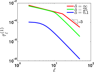
Figure 2: (color online) Dimensionless relaxation times of the Lennon Brochard mode $\bar{\tau}^{(1)}_{\ell}$ for an elastic membrane vs the mode number $\ell$ for various permeation parameters $\bar{\alpha}$. The dimensionless elastic parameters of the membrane are $\bar{\mu}=75$ and $\bar{K}=225$, which corresponds to the Poisson ratio $\sigma=0.5$ and the radius to thickness ratio $R/h=5$. $\bar{\tau}^{(1)}_{\ell}=0$ for $\bar{\alpha}=0$ for all $\ell$.

All three cases correspond to a perfectly elastic membrane so that $\bar{\mu}$ and $\bar{K}$ are real and frequency independent. For $\ell\gg 1$ the characteristic wavelength of the deformation is much smaller than the radius of curvature of the sphere so we should expect to recover the flat membrane result of Lennon and Brochard Brochard:75 . Indeed, for large $\ell$, we find that, $\bar{\tau}_{\ell}^{(1)}\sim\ell^{-3}$ so that the decay rate $\left(\bar{\tau}_{\ell}^{(1)}\right)^{-1}\sim\ell^{3}\sim\left(\frac{R}{\lambda}\right)^{3}\sim q^{3}$ where $\lambda$ is the wavelength of the mode. As expected based on our analysis of the plane permeable membrane, the transition to the Lennon and Brochard behavior is more apparent for the impermeable case ($\bar{\alpha}=\infty$) and becomes less distinct as $\bar{\alpha}$ decreases. It is not possible to consider the case $\bar{\alpha}=0$ when discussing the relaxational dynamics of the LB mode as the decay rate of this mode becomes infinite as $\bar{\alpha}\to 0$ for all $\ell$.

We parameterize the relative degree of bending versus compression associated with these modes by introducing their ratio

$$w_{\ell m}/\Psi_{\ell m}=Z^{(p)}(\ell),$$ (54)

where $p=1,2$ indexes the two linearly independent modes of the system. We plot in Fig. 3 this ratio $Z^{(1)}(\ell)$ for the first mode whose corresponding decay times are shown in Fig. 2 . Examining this plot it is clear that this mode is, indeed, the analogue of the Lennon–Brochard bending mode since $|Z^{(1)}(\ell)|\gg 1$. This identification of the first mode with bending becomes more exact at higher $\ell$ where the curvature of the membrane becomes less significant for the dynamics. The overall negative sign for this result is due to the fact that where the membrane bends outward the material expands and where it curves inward the material compresses. Due to the overwhelming bending character of this mode we will refer to it as the Lennon–Brochard (LB) mode.

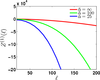
Figure 3: (color online) Ratio of bending to stretching $Z^{(1)}(\ell)$ in the Lennon-Brochard mode vs. mode number $\ell$ of a perfectly elastic membrane. The membrane elasticity parameters are identical to those used in Fig. 2. The values of the dimensionless permeation coefficient are listed in the figure legend.

We now turn to the second mode and plot in Fig. 4 its dimensionless decay time $\bar{\tau}_{\ell}^{(2)}=1/i\omega^{(2)}_{\ell}$ as a function of $\ell$. We use the same elastic parameters $\bar{\mu}$ and $\bar{K}$, as in the plot of the decay times of the LB mode and show curves corresponding to an impermeable case ($\bar{\alpha}=\infty$), one of intermediate permeability ($\bar{\alpha}=25$), and a case where the fluid passes through the membrane without any resistance ($\bar{\alpha}=0$).

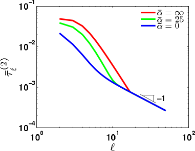
Figure 4: (color online) Dimensionless relaxation time $\bar{\tau}^{(2)}_{\ell}$ in the longitudinal sound mode vs. the mode number $\ell$ for purely elastic membranes having various dimensionless permeation parameters $\bar{\alpha}$. The dimensionless elastic parameters of the membrane are $\bar{\mu}=75$ and $\bar{K}=225$ as in Fig. 2.

When $\ell\gg 1$ all these cases converge onto a single curve so that $\bar{\tau}_{\ell}^{(2)}\sim\ell^{-1}$ independent of $\bar{\alpha}$.

As $\bar{\tau}_{\ell}^{(2)}\sim\ell^{-1}$ for large $\ell$, this mode cannot be controlled by membrane bending at high wavenumber. Turning to $Z^{(2)}(\ell)$ – see Eq. (54) –, which we plot in Fig. 5, we see that this mode is dominated by the in-plane compression of the membrane. In fact, this mode is the remnant of longitudinal sound (LS) in the elastic membrane that is over-damped due to the coupling to the surrounding solvent. It is interesting to note that only at large $\ell$ the (LB) mode becomes strongly bending dominated while the longitudinal sound mode (LS) only loses its bending character at large $\ell$.

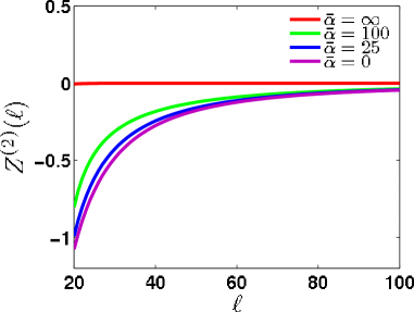
Figure 5: (color online) Ratio of bending to stretching $Z^{(2)}(\ell)$ in the longitudinal sound mode vs. mode number $\ell$ of a perfectly elastic membrane. The membrane elasticity parameters are identical to used in Fig. 4. The values of the dimensionless permeation coefficient are listed in the figure legend.

It is well known that bending and longitudinal sound are orthogonal normal modes of the linearized membrane/solvent system in the case of flat membrane Levine:02 . Examining the results for the sphere we find that geometry couples these deformations, but, at high wave number (or large $\ell$) where the wavelength of the deformation is much less than the radius of curvature $R$, the two orthogonal modes of the sphere approach the simple mode structure of the flat membrane.

Before closing our discussion of the mode structure of the spherical elastic membrane, we must consider the $\ell=0$ mode of the membrane, which corresponds to purely radial motion of its surface. This mode must be handled independently of the others because of the incompressibility of the solvent. Because of that incompressibility, there can be no corresponding radial motion of the solvent so that the membrane relaxes against a background of quiescent fluid. In this mode the radial deformation obeys

$$\frac{\partial w}{\partial t}=-\frac{k_{\rm eff}}{\alpha}\,w,$$ (55)

with no angular dependence, and with an effective spring constant of

$$k_{\rm eff}=4\bigg{[}\frac{\kappa+R^{2}K}{R^{4}}\bigg{]}.$$ (56)

The dimensionless relaxation rate of the $\ell=0$ LB mode is then given by Eqs. (55) and (56). We find

$$\bar{\tau}_{0}^{(2)}=\frac{\bar{\alpha}}{4}\,\frac{1}{1+\bar{K}}.$$ (57)

It is clear that the decay rate of this mode vanishes in the limit of an impermeable ($\bar{\alpha}=\infty$) sphere as volume changing deformations are not allowed. As the sphere becomes more permeable the decay rate increases becoming infinite in the limit of a “ghost membrane” ($\bar{\alpha}=0$) since we have neglected the membrane’s inertia.

To compare these results with experiments it is useful to recognize that our two-dimensional solid membrane is an idealization of a thin sheet of thickness $h$ whose material properties can be defined in terms of three-dimensional Lamé coefficients $\mu_{3}$, $\lambda_{3}$. Using standard results Landau:59 ; Komura:92 we may then reexpress our dimensionless elastic parameters in terms of the geometry of the system and the Poisson ratio of the membrane material $\sigma$. We find

$$\bar{\mu} = 6\left(\frac{R}{h}\right)^{2}(1-\sigma)$$ (58)

$$\bar{K} = 6\left(\frac{R}{h}\right)^{2}(1+\sigma),$$ (59)

while the bending modulus is given by

$$\kappa=\frac{\mu_{3}h^{3}}{3}\,\frac{\lambda_{3}+\mu_{3}}{\lambda_{3}+2\mu_{3}}$$ (60)

We return to this point with regard to the microrheology of viscoelastic spherical membranes in section III.

III The nanoindentation response function

Using the above analysis of the mechanics of porous, viscoelastic spherical shells, we now determine the microrheological signature of viscoelastic, porous shells. As discussed above, these results are relevant to the study of the mechanics of viral capsids, colloidosomes, and porous lipid bilayers such as those that contain membrane-bound pore-forming proteins.

In the active AFM-based mechanical measurement, the shell is deformed by antipodally applied forces directed radially toward the center of the shell. To measure the mechanics of the shell the distance between the point of force application and its antipode is measured. This distance, due to the application of a sinusoidally varying force $F_{0}e^{-i\omega t}$, will deviate from the shell diameter with an amplitude

$$D(\omega)=2R-H(\omega)F_{0},$$ (61)

which defines the response function $H(\omega)$. In the passive microrheological experiment, on the other hand, the thermally excited fluctuations of $2R-D$ give the same information via the fluctuation-dissipation theorem Mason:95 ; Levine:00 .

To calculate $H(\omega)$ we apply equal and opposite forces to the “north” and “south” poles of the sphere, i.e. at polar angles $\theta=0,\pi$. The force balance boundary condition Eq. (41) then becomes

$$\hat{\bm{r}}\cdot\bm{F}_{\rm fluid}+\bm{\pi}_{1}{(\omega)}+\bm{\pi}_{2}{(\omega)}=\hat{\bm{r}}\cdot\bm{F},$$ (62)

where $\bm{\pi}_{1,2}$ are the external normal stresses on the surface

$$\bm{\pi}_{1}(\omega) =-\delta(\theta)e^{-i\omega t}\,\hat{\bm{r}}\,F_{0}/a^{2}$$ (63)

$$\bm{\pi}_{2}(\omega) =\delta(\theta-\pi)e^{-i\omega t}\,\hat{\bm{r}}\,F_{0}/a^{2}.$$ (64)

As shown above we will consider point forces so that the area of the sphere contacted by the AFM tip $a\to 0$ at constant $F_{0}/a^{2}=\pi_{0}$. Using the completeness of spherical harmonics on the unit sphere we express these externally applied stresses in terms of spherical harmonic modes:

$$\bm{\pi}(t,\theta,\phi)=-\hat{\bm{r}}\,\pi_{0}\sum_{\ell,m}\left[Y^{*}_{\ell 0}(0,0)+Y^{*}_{\ell 0}(\pi,0)\right]Y_{\ell m}(\theta,\phi)e^{-i\omega t}.$$ (65)

Thus the AFM-induced pinching of the shell couples to all the spherical harmonic modes of the system discussed above. The effect of the finite-size of the AFM tip can be accounted for by putting in a large-$\ell$ cutoff in the sum shown in Eq. (65). For reasonably small tip, this effect must be negligible. Using these previous results we compute the radial deformation amplitude associated with each $\ell-$mode at the north pole of the sphere. In terms of the dimensionless frequency, $\bar{\omega}=\omega\eta R^{3}/\kappa$, this radial displacement of the sphere at the north pole is given by

$$w_{\ell}(\bar{\omega})=2\frac{R^{4}}{\kappa}\pi_{0}[1+(-1)^{\ell}]Y^{*}_{\ell 0}(0,0)\zeta_{\ell}(\bar{\omega}),$$ (66)

where $\zeta_{\ell}(\bar{\omega})$ is the frequency-dependent complex radial compliance of the shell due to a radially applied normal stress distributed over the sphere as $Y_{\ell 0}(\theta)$. This compliance results from both the Lennon-Brochard (LB)and longitudinal sound (LS) modes of the shell discussed above. The complex, frequency-dependent response function can be expressed in terms of five dimensionless functions of the angular momentum of the mode $\ell$:

$$\zeta_{\ell}(\bar{\omega})=\frac{\Lambda_{1}(\ell)+i\,\bar{\omega}\,\Lambda_{2}(\ell)}{\Lambda_{3}(\ell)+i\,\bar{\omega}\,\Lambda_{4}(\ell)+\bar{\omega}^{2}\,\Lambda_{5}(\ell)},$$ (67)

where due to their length, these functions $\Lambda_{1}(\ell),...,\Lambda_{5}(\ell)$ are reported in Appendix D. As shown there, it is through these functions that the $\ell-$dependent response function acquires its dependence on the dimensionless permeation parameter $\bar{\alpha}$ and on the elastic constants of the membrane written in terms of the ratio $R/h$ and the Poisson ratio $\sigma$ as shown in Eqs. (58) and (59).

Summing over the $\ell-$ modes using Eqs. (65) and (66) we find the radial displacement of the shell at $(\theta,\phi)$ to be

$$w(\bar{\omega},\theta,\phi)=\frac{\pi_{0}R^{4}}{\kappa}\sum_{\ell=0}^{\infty}Y_{\ell 0}(\theta,\phi)[1+(-1)^{\ell}]\zeta_{\ell}(\bar{\omega})Y^{*}_{\ell 0}(0,0).$$ (68)

Thus the amplitude of oscillations of the diameter is given by

$$D(\bar{\omega})=2R+w(\bar{\omega},0,0)+w(\bar{\omega},\pi,0).$$ (69)

Using the definition in Eq. (61) and Eqs. (67), (68), and (69 ), we solve for the response function in terms of the point force response of the shell. We find that the diameter response function is given by

$$H(\bar{\omega})=\frac{2R^{4}}{\kappa}\sum_{\ell=0}^{\infty}[1+(-1)^{\ell}]\zeta_{\ell}(\bar{\omega})|Y_{\ell 0}(0,0)|^{2}.$$ (70)

III.1 An elastic shell

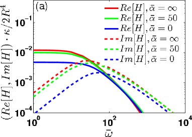
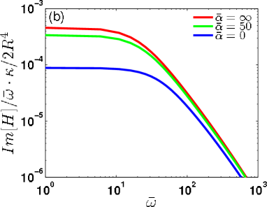
Figure 6: (color online) The response function of a porous, elastic shell. In panel (a) we plot the real (${\rm Re}[H(\bar{\omega})]$, solid lines) and imaginary (${\rm Im}[H(\bar{\omega})]$, dashed lines) parts of the response function vs dimensionless frequency $\bar{\omega}$ for various values of the permeation parameter $\bar{\alpha}$. The remaining material parameters are: $R/h=5$, Poisson ratio $\sigma=0.5$. In panel (b) we show the thermal power spectrum (${\rm Im}[H(\bar{\omega})]/\bar{\omega}$) using the same material parameters.

We plot in Fig. 6(a) the real (in phase) and imaginary (out of phase) parts of the diameter response function $H(\bar{\omega})$ for purely elastic shells of varying porosity. In anticipation of future fluctuation-based microrheology experiments we plot in Fig.5(b) the predicted power spectra for the thermal fluctuations of this variable, computed using the fluctuation-dissipation theorem Landau:51 . Examining the figure we note that the response function can be characterized as having a low-frequency elastic plateau followed by a cross-over to a viscous-dominated decay at high frequencies. As the dimensionless permeation coefficient is varied from that of an impermeable shell ($\bar{\alpha}=\infty$) to one that allows fluid permeation with no resistance ($\bar{\alpha}=0$), the dimensionless cross-over frequency moves from $\approx 10$ to $\approx 10^{2}$. We return to predicted values of this cross-over frequency for various physical systems in section IV. Within the low-frequency plateau where much, if not all, the dynamical data is likely to be taken, the main effect of permeation is to shift the value of the response function by approximately a factor of two. Thus, in order to correctly extract the bending and compression moduli of the shell to better than this factor of two, an accurate account of the permeation must be made. In the passive microrheology experiment, the effect of permeation on the thermal power spectrum of diameter fluctuations is more pronounced. Ignoring permeation in this sort of measurement leads to quantitative inaccuracies on the order of $4$ as shown in Fig. 6(b). We now consider the case of a viscous shell.

III.2 A viscous shell

The case of a viscous shell can be physically realized with giant unilamellar vesicles (GUVs) that contain pore-forming transmembrane proteins or protein complexes. This system allows for the largest variation of permeation coefficients of any that we study. By varying the number of such proteins in these protein/lipid complexes, one may vary the porosity parameter from essentially $\bar{\alpha}=\infty$ (no pore-forming protein) to finite values. Using the solution for the permeation coefficient found in Appendix A, it should be possible to reach values of $\bar{\alpha}=10$ for the lipid vesicle systems.

To determine the dynamics of a purely viscous shell we replace real, frequency-independent shear modulus of the shell by a viscous response: $\mu\to-i\omega\eta_{\rm m}$, with $\eta_{\rm m}$ being the two-dimensional surface viscosity of the the membrane or bilayer. To allow any radial deformations of the impermeable bilayer, there must be some area change of the surface. One may imagine that the surface of a tensed GUV is essentially inextensible, however, even such

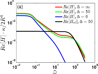
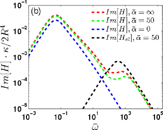
Figure 7: (color online) Response function of a GUV containing pore-forming protein complexes. In panels (a) and (b) we show the real (${\rm Re}[H(\bar{\omega})]$) and imaginary (${\rm Im}[H(\bar{\omega})]$) parts of the response function vs. dimensionless frequency $\bar{\omega}$ respectively using various values of the permeation parameter $\bar{\alpha}$. The other dimensionless parameters were:$R/h=20$, $\sigma=0.5$ $\eta_{\rm m}/R\eta=0.1\bar{\mu}_{0}$, $\bar{\mu}_{0}$ and $\bar{K}$ defined in Eqs. (58) and (59). For comparison, black solid line shows the real part of the response function for an elastic shell with $R/h=20$, $\sigma=0.5$, $\bar{\alpha}=50$. The black dashed line corresponds to the imaginary part of the response function of an elastic shell with the same material parameters as in panel (a). In (c) we plot the thermal power spectrum (${\rm Im}[H(\bar{\omega})]/\bar{\omega}$) as a function of the dimensionless frequency $\bar{\omega}$ using the same material parameters as in panel (a). Black line – elastic shell.

tensed structures contain a reservoir of extra area hidden in the (small-scale) thermal undulations of the surface Milner:87 ; Kaizuka:04 . Thus the two-dimensional bulk modulus of the viscous shell is dominated by a large, but finite elastic component. We expect that there may well be a dissipative or viscous response of the shell to area-changing deformations, but we ignore these subdominant corrections. In Fig. 7(a), we plot the real and imaginary parts of the response function for a porous ($\bar{\alpha}=50$), purely viscous shell with a finite area compression modulus, $\bar{K}$. In part (b) of the same figure, we calculate the power spectrum of thermal fluctuations of the diameter of such an object.

The low frequency response of the porous, viscous membrane exhibits an elastic plateau due to its elastic response to both bending and compression. The viscous shell, however, admits a new intermediate frequency response regime associated with viscous dissipation within the fluid membrane. In this intermediate frequency regime, the real part of the response function decays as $\bar{\omega}^{-0.66}$ over about two decades in frequency. Examining these results we note that there are dramatic qualitative differences between the response functions of viscous and elastic shells at least within this intermediate frequency range.

In Fig. 7(b) we see the low-frequency peak in the imaginary part of the response function associated with these internal (to the membrane) shear modes. At still higher frequencies, both the real and imaginary parts of the response function are dominated by dissipative stresses due to solvent flow and permeation through the pores. This can be most easily seen in the correspondence of the high-frequency peak of the imaginary part of response function of the viscous membrane with only peak in the corresponding part of the response function for the purely elastic shell. In this high frequency limit a viscous membrane and an elastic shell show essentially an identical mechanical response. This is reasonable since the high-frequency dynamics of both systems are dominated by solvent flow and permeation.

Passive microrheological measurements at low frequencies can easily distinguish between a viscous and an elastic shell as can be see by the difference between their power spectra shown in Fig. 7(c). The effect of permeation, as can be seen by comparing the curves, is principally in shifting the hight of the plateau region and slightly altering the transition frequency to the solvent-dominated, high-frequency regime.

III.3 Viscoelastic shells

To explore the role of viscoelasticity in the mechanics of a porous spherical shell, we consider two archetypal cases. We first calculate the response function for a viscoelastic shell where the shear modulus has a single relaxation time, $\tau_{s}$. This Maxwell model Bird:77 of the shear modulus can be written as

$$\bar{\mu}(\bar{\omega})=\bar{\mu}_{0}\,\frac{-i\bar{\omega}\bar{\tau}_{s}}{1-i\bar{\omega}\bar{\tau}_{s}},$$ (71)

where $\bar{\tau}_{s}$ is the dimensionless shear stress relaxation time. Deformations occurring at a frequency scale much lower than the inverse stress relaxation time relax viscously. The high frequency dynamics, on the other hand, see an elastic shear response of the material with shear modulus $\bar{\mu}_{0}$.

In Figs. 8(a) and (b) we plot the real and imaginary parts of the response function respectively for a viscoelastic shell having a complex, frequency-dependent shear modulus of the Maxwell form. We take the shear stress relaxation time $\bar{\tau}_{s}$ to be within the range of decay times of the various $\ell-$modes of the system. Thus, the small $\ell-$modes of the shell

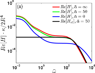
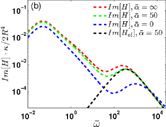
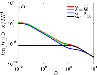
Figure 8: (color online) The response function of a shell with a viscoelastic shear modulus. In panels (a) and (b) we show the real (${\rm Re}[H(\bar{\omega})]$) and imaginary parts of the response function vs. dimensionless frequency $\bar{\omega}$ respectively using various values of the permeation parameters $\bar{\alpha}$. The other dimensionless parameters were: $R/h=20$, $\sigma=0.5$, $\bar{\tau}_{s}=0.1$, $\bar{\mu}_{0}$ and $\bar{K}$ defined in Eqs. (58) and (59). For comparison, the black lines shows the real (solid) and imaginary (dashed) parts of the response function for an elastic shell with $R/h=20$, $\sigma=0.5$, $\bar{\alpha}=50$. In (c) we plot the thermal power spectrum (${\rm Im}[H(\bar{\omega})]/\bar{\omega}$) as a function of the dimensionless frequency $\bar{\omega}$ using the same material parameters as in panel (a). Black line – purely elastic shell.

have long decay times relative to the stress relaxation time and thus experience viscous relaxation dynamics, where the higher $\ell-$modes of the system decay fast enough to be affected by the elastic shear response of the system.

It is that for a viscoelastic shell the intermediate frequency response regime associated with the viscous system remains, but the frequency dependence of the real part of the response function is weakened: $\sim\bar{\omega}^{-0.44}$. This appears reasonable as the viscoelastic case effectively interpolates between the response of an elastic shell (high $\ell$-modes) and a viscous one (low $\ell$-modes). The slope of the real part of the response function (see Fig. 8(a)) in the intermediate response regime now is $\bar{\alpha}$-dependent. Thus, to use the response function to extract properties of the viscoelastic response of the shell is difficult without an accurate model of solvent permeation through it.

In Fig. 8(c) we plot the thermal power spectrum for this model. As long as the shear stress relaxation rate is small compared to the cross-over to the high-frequency terminal behavior of the system, it is indeed possible to observe the viscoelastic response of the shell by examining the thermal power spectrum. This identification, however, relies on a separation of time scales so that $\bar{\tau}_{s}$ remains long compared to the cross-over timescale to viscous-dominated behavior. As we discuss in section IV, this separation of time scales should be easy to achieve in many physical systems.

Finally, we study perhaps the most potentially interesting example of a viscoelastic shell on the nanoscale. In some viral capsids the individual capsomeres can undergo a conformational change that changes their effective cross-sectional area. These internal degrees of freedom related to volume-changing allosteric transitions of the proteins making up the shell of the virus allow for new dissipation associated with area-changing deformations. To model this system we include a complex frequency-dependent two-dimensional bulk modulus of the form

$$\bar{K}(\bar{\omega})=\bar{K}_{0}\left[1+g\frac{-i\bar{\omega}\bar{\tau}_{B}}{1-i\bar{\omega}\bar{\tau}_{B}}\right],$$ (72)

where $\bar{K}_{0}$ sets the overall modulus scale, $\bar{\tau}_{B}$ is the inverse rate of conformational change, and $g\bar{K}_{0}$ sets the maximum of the dissipative part of the modulus at $\bar{\omega}\bar{\tau}_{B}\simeq 1$.

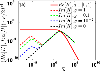
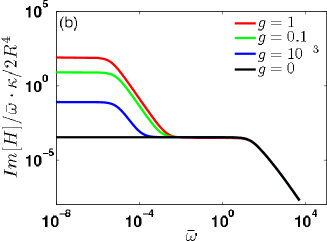
Figure 9: (color online) A simple mechanical model of a viral capsid in which the capsomers undergo a cross-sectional area changing allosteric transition. In panel (a) we plot the real and imaginary parts of the response function for different Maxwell solid models of the shell – see Eq. (72). In panel (b) we plot the expected thermal power spectrum (${\rm Im}[H(\bar{\omega})]/\bar{\omega}$). In all cases the material parameters of the shell are given by: $R/h=5$, $\tau_{B}=10^{-3}$s, $Y=140$MPa, $\sigma=0.5$, $\bar{\alpha}=50$.

The typical time scale for allosteric transition in proteins is on the order of microseconds to milliseconds. The ratio of the zero-frequency elastic part of the area modulus $\bar{K}_{0}$ to the dissipative contribution at the frequency of these allosteric transitions is controlled by the constant $g$. Since we know of no quantitaive measurement of these parameters, we sweep the value of $g$ from zero, which corresponds to a purely elastic shell as shown in Fig. 6, to $g=1$, where this dissipative contribution to the stress dominates the zero-frequency elastic contribution to the area modulus. It is clear from Fig. 9 that even a small dissipative response to compressive stresses at time scales associated with allosteric transitions leads to a clear and measurable change in the response function of the shell.

IV Summary and Discussion

We have developed a theoretical model for the dynamics of a porous spherical shell immersed in a viscous solvent and used it to examine the utility of nanoindentation-based rheological measurements. In the limit of a flat, porous membrane immersed in a viscous solvent, we calculated the relaxational dynamics of the bending or undulatory modes of the surface. These modes are well-understood in the limit of a impermeable surface. In that limiting case, the long-range hydrodynamic flows introduce a nonlocal coupling of the stress and displacement along the surface. It has long been known that the hydrodynamic coupling shifts the dispersion relation of the undulation modes of wavevector $q$ from their expected “local drag” form of $\omega\sim-iq^{4}$ to correct answer of $\omega\sim-iq^{3}$ incorporating the hydrodynamic cooperativity of the system as first proposed by Lennon and Brochard Brochard:75 . For the case of permeable membrane, the dispersion relation of the undulatory modes smoothly crosses over from the local drag form to the usual Lennon-Brochard solution as the wave number is varied. The cross-over length is set by $\ell\sim\eta/\alpha$. At lengths much larger than $\ell$ the solvent permeation generates a subdominant correction to the usual dynamics of the undulatory modes of a membrane. Below this length, however, permeation effectively destroys the hydrodynamic coupling along the membrane leading to a new dynamics consistent with the naïve, local-drag approximation.

In order to consider the mechanics of spherical permeable membranes (of radius $R$), we examined both compression and bending deformations of the material since curvature couples these linearly independent modes of the flat membrane. The hydrodynamic interactions of the membrane are also less simple in this geometry. Using a solution for the solvent dynamics both inside and outside the spherical shell, we determined the over-damped normal modes of the system. Owing to the spherical symmetry of the problem, these modes are proportional to the spherical harmonics and thus can be indexed by the usual angular momentum variables, $(\ell,m)$. At small angular momentum, i.e. $\ell\sim 1$, the two linearly independent modes of the membrane each combine an undulatory and compressional character. At higher angular momentum corresponding to higher wavevectors on the surface $q\sim\ell/R$, the dynamics approach those of the flat interface where these two modes acquire a dominantly undulatory or compressional character respectively. Using this short length scale behavior, we label the modes as either the Lennon-Brochard (i.e. undulatory) or compressional type.

We use these dynamical calculations to study the expected finite-frequency response of a variety of essentially spherical, viscous, elastic, and viscoelastic porous shells. Such systems include colloidosomes, nanoparticle networks, vesicles containing membrane-bound pore-forming protein complexes, and viruses. The principal questions that we address are how does porosity affect the mechanical response of viscous, elastic, and viscoelastic spherical shells and specifically, for the case of viral capsids, is it possible to mechanically detect allosteric transitions in the capsomeres making up the proteinous outer shell of a virus?

To address these questions, we need only determine the characteristic frequencies associated with the nondimensionalized curves shown in Figs. 6, 7, 8, and 9. A few general comments are in order. First, the characteristic frequency associated with the transition between the low-frequency plateau and high-frequency, fluid dominated decay of the response function is typically large enough in viruses to render the high-frequency region unobservable using current methods. Expressing the frequencies $f$ in dimensional form using the dimensionless angular frequency $\bar{\omega}$ and the relation

$$f=\bar{\omega}\left[\frac{Y}{24\pi\,\eta(1-\sigma^{2})}\right](h/R)^{3},$$ (73)

we find that the characteristic cross-over frequency for a CCMV virus Michel:06 to be on the order of $10^{8}$Hz. For a larger and mechanically softer liposome, however, this transition frequency is $\sim 100$kHz. For colloidosomes and other synthetic structures on the scale of one to ten microns we estimate this transition frequency to be $\sim 10^{2}-\,10^{4}$Hz. The general trends are simple to understand from Eq. (73). Larger (large $R$) and thinner-walled (small $h$) spheres have a lower transition frequency, while those spheres made of less elastically compliant materials (i.e. higher Young’s modulus $Y$) have higher transition frequencies.

We expect, based on the above estimates, that the transition to a permeation-dominated response is not observable in viral capsids. One advantage of this point is that an observed increase in the imaginary (out-of-phase) response function for viral capsids implies the existence of internal dissipative modes of the structure that are likely to be related to allosteric transitions of capsomeres or in their rearrangement relative to one another. We show in Figs. 8,9 two possible rheological signatures of such internal dissipative modes. In the former we suppose that there is a large elastic response of the shell to area-changing deformations, but that the shear response of the material is viscoelastic. One might expect such a mechanical response if the individual capsomeres irreversibly rearrange in response to applied stress. In the latter case we explore a system having a Maxwell solid response to area compression, but an elastic response to shear. Such a material response might be expected if the individual capsomeres undergo allosteric transitions that change their effective cross-sectional area. In Fig. 8, we see that the Maxwell shear response leads to measurable corrections to the rheological spectrum of the object.

The AFM-based mechanical probe is also highly sensitive to a viscoelastic response of the area compression modulus as might be due to allosteric transitions in the capsomeres. The expected separation of time scales between the lower frequency allosteric transitions ($10^{3}$Hz to $10^{6}$Hz) and transition to permeation dominated dynamics ($10^{8}$Hz) demonstrates that this measurement is well-suited to exploring such capsomere conformational changes.

The permeation parameter is not irrelevant for making quantitative measurements. This parameter shifts the value of the elastically dominated low-frequency plateau of elastic shells (such as viruses) by as much as a factor of four. This dynamical response function is principally controlled by the bending modulus of the shell so that AFM-based measurements of that quantity can be in error by as much as a factor of ten if permeation is neglected in the interpretation of the data. The effect of solvent permeation is generically more important in systems that are both larger and mechanically more compliant. Thus the effect of solvent permeation can play a large role in the mechanical response of large GUVs containing pore-forming proteins.

The combined effects of solvent permeation and viscoelasticity remains to be fully explored in a wide variety of biological and synthetic nanoscale shells and vesicles. Based on our present work, accounting for solvent permeation will be important for the quantitative interpretation of such rheological data. By taking such effects into account it may be possible to make sensitive measurements of the collective effects of protein conformational change in viral capsids and to probe the mechanics of a number of other similar structures.

Appendix A The permeation coefficient

To determine the permeation coefficient we treat the porous membrane of thickness $t$ as having an array of pores or radius $r_{0}$. We use the well-known result for the fluid flux $Q$ through such a tube of length $t$ and radius $r_{0}$ due to a pressure difference $\Delta P$ across the tube to write Lamb:32

$$Q=\frac{\pi r_{0}^{4}}{8\eta}\frac{\Delta P}{t}.$$ (74)

We then suppose that the number of such tubes is $k$ per unit area of the membrane and assume that the total flux through these tubes is simply additive. Then the total flux through the area $L^{2}$ is thus given by

$$\mbox{total flux}=kL^{2}Q,$$ (75)

and the average velocity of fluid coming out of the membrane is

$$v_{av}=k\frac{\pi r_{0}^{4}}{8\eta}\frac{\Delta P}{t}.$$ (76)

On the other hand, we assert from Darcy’s law that

$$v_{av}=\frac{\Delta P}{\alpha}.$$ (77)

From Eqs. (76) and (77) we find the permeation coefficient to be given by

$$\alpha=\frac{8\eta t}{\pi r_{0}^{4}k}.$$ (78)

Expected values of the permeation coefficient for a variety of micron and nanoscale hollow, porous shells are given in Table 1. In the text we introduce a dimensionless form of the permeation coefficient $\bar{\alpha}$ that is defined by

$$\bar{\alpha}\equiv\frac{\alpha\cdot R}{\eta}=\frac{8\,R\,t}{\pi r_{0}^{4}\,k},$$ (79)

where $R$ is radius of the sphere and $\eta$ the viscosity of the surrounding solvent.

Appendix B Undulations of a plane permeable membrane

We calculate the fluid flow associated with the undulations of a permeable membrane. To begin we look for solutions of the incompressible Stokes equation

$$\bm{\nabla}\cdot{\bf v}=0$$ (80)

$$\displaystyle\rho\frac{\partial{\bf v}}{\partial t}=\eta\nabla^{2}{\bf v}-\bm{\nabla}p.$$

driven by sinusoidal membrane undulations of the form

$$w=w_{q}e^{iqx-i\omega t}.$$ (81)

These undulations apply an external normal stress on the fluid at the membrane located in the $xy$ plane ($z=0$) of the form

$$\pi_{e}=\pi e^{iqx-i\omega t}.$$ (82)

Correspondingly, we expect a solution for the fluid velocity field ${\bf v}$ and pressure $p$ of the form

$${\bf v}={\bf v}(z)e^{iqx-i\omega t}$$ (83)

$$p=p(z)e^{iqx-i\omega t},$$ (84)

but the fluid velocity and pressure fields must vanish far from the membrane $z\to\pm\infty$ and satisfy at the membrane

$$v^{+}_{x}(0)=v^{-}_{x}(0)=0$$ (85)

$$v_{z}^{+}(0)=v_{z}^{-}(0)$$ (86)

Additionally, the fluid incompressibility condition gives

$$\frac{\partial v_{z}}{\partial z}+v_{x}(z)iq=0.$$ (87)

Using these in Eq. (B) equation we find

$$-\rho\,i\omega\,v_{x}(z)=\eta\left(-q^{2}v_{x}+\frac{\partial^{2}v_{x}}{\partial z^{2}}\right)-i\,q\,p(z)$$ (88)

$$-\rho\,i\omega\,v_{z}(z)=\eta\left(-q^{2}v_{z}+\frac{\partial^{2}v_{z}}{\partial z^{2}}\right)-\frac{\partial p(z)}{\partial z}$$ (89)

The general form of the solutions to these ordinary differential equations is

$$v_{x}(z)=ae^{\lambda z}\quad v_{z}(z)=be^{\lambda z}\quad p(z)=ce^{\lambda z},$$ (90)

where the incompressibility condition Eqs. (80) and (87) requires that the undetermined constants are related by

$$b=-\frac{iq}{\lambda}a,$$ (91)

while Eqs (88) and (89) give four solutions

$$\lambda^{2}=q^{2},\,q^{2}-i\frac{\rho\omega}{\eta}.$$ (92)

Using the boundary conditions we find solutions of the form

$$v_{x}^{\pm}(z) =\mp iqA(e^{\mp qz}-e^{\mp lz})e^{iqx-i\omega t}$$ (93)

$$v_{z}^{\pm}(z) =qA(e^{\mp qz}-\frac{q}{l}e^{\mp lz})e^{iqx-i\omega t}$$ (94)

$$p^{\pm}(z) =\mp i\omega\rho Ae^{\mp qz}e^{iqx-i\omega t},$$ (95)

with $l=\sqrt{q^{2}-i\rho\omega/\eta}$.

Knowing the pressure and velocity fields, we require force balance at the membrane:

$$(\sigma_{zz}^{-}-\sigma_{zz}^{+})+\pi=\kappa\nabla^{4}w,$$ (96)

using the fluid stress tensors and membrane bending modulus discussed in the text.

The permeability of the membrane sets the velocity difference between the fluid and the membrane at $z=0$. Thus we also have

$$\alpha\left(v_{z}(0)-\frac{dw}{dt}\right)=(p^{-}-p^{+}).$$ (97)

These conditions set the two remaining unknown constants above, $A$ from Eqs. (93)-(95) and $w_{q}$ by requiring nontrivial solutions to the set of algebraic equations

$$A\left[\alpha q\left(1-\frac{q}{l}\right)-2\,i\omega\rho\right]+w_{q}\,\alpha\,i\omega=0$$

$$A\,2i\omega\rho-\kappa q^{4}w_{q}=-\pi.$$ (98)

Working in the limit where fluid inertia is irrelevant $\omega\rho\ll\eta q^{2}$ and solving for $w_{q}$ we find

$$w_{q}=-\frac{\pi\,\left[\frac{\alpha}{2q\eta}+2\right]}{2i\omega\alpha-\kappa q^{4}\,\left[\frac{\alpha}{2q\eta}+2\right]}$$ (99)

as discussed in the text.

Appendix C The A matrix

The eigenvectors and eigenvalues of the $A$ matrix defined by Eq. (52) determine the relaxation times and mode structure of the coupled membrane deformation and solvent flow modes. The components of this matrix are listed below:

$$A_{11}=(2\ell+1)(4\ell^{3}+6\ell^{2}-\ell+3)\bar{\alpha}$$

$${}-(\ell-1)^{2}(\ell+2)^{2}(2\ell+1)(4\ell^{3}+6\ell^{2}-\ell+3)\frac{1}{i\,\bar{\omega}_{\ell}}$$

$${}-(\ell-1)^{2}\ell(\ell+1)(\ell+2)^{2}(2\ell+1)\frac{\bar{\alpha}}{i\,\bar{\omega}_{\ell}}$$

$${}-4(2\ell+1)(4\ell^{3}+6\ell^{2}-\ell+3)(2\ell+1)\frac{\bar{K}}{i\,\bar{\omega}_{\ell}}$$

$${}-2\ell(\ell+1)(\ell+2)\frac{\bar{\alpha}\,\bar{K}}{i\,\bar{\omega}_{\ell}},$$

$$A_{12}=\ell(\ell+1)\Bigl{[}-3(2\ell+1)\bar{\alpha}$$

$${}+2\,(2\ell+1)(4\ell^{3}+6\ell^{2}-\ell+3)\frac{\bar{K}}{i\,\bar{\omega}_{\ell}}$$

$${}-3(\ell-1)\ell(\ell+2)\frac{\bar{\alpha}\,\bar{\mu}}{i\,\bar{\omega}_{\ell}}\Bigr{]},$$

and

$$A_{21}=-3(2\ell+1)\bar{\alpha}$$

$${}+2(\ell-1)^{2}(\ell+2)^{2}(2\ell+1)\,\frac{1}{i\,\bar{\omega}_{\ell}}$$

$${}-3(\ell-1)^{2}\ell(\ell+2)^{2}\,\frac{\bar{\alpha}}{i\,\bar{\omega}_{\ell}}$$

$${}+12(2\ell+1)\,\frac{\bar{K}}{i\,\bar{\omega}_{\ell}}$$

$${}+2\ell(\ell+2)(2\ell-1)\frac{\bar{\alpha}\bar{K}}{i\,\bar{\omega}_{\ell}}$$

$$A_{22}=\ell(2\ell+1)(4\ell^{2}+6\ell-1)\bar{\alpha}$$

$${}-6\ell(\ell+1)(2\ell+1)\frac{\bar{K}}{i\,\bar{\omega}_{\ell}}$$

$${}-\ell^{2}(\ell+1)(\ell+2)(2\ell-1)\,\frac{\bar{\alpha}\bar{K}}{i\,\bar{\omega}_{\ell}}$$

$${}-(\ell-1)\ell(\ell+2)(2\ell^{2}+3\ell+4)\,\frac{\bar{\alpha}\bar{\mu}}{i\,\bar{\omega}_{\ell}}.$$

Appendix D The response function

Here we list the $\ell$ dependence of each function entering into the diameter response function shown in Eq.(67). These functions depend also on the dimensionless permeation parameter $\bar{\alpha}$, dimensionless shear modulus $\bar{\mu}$ and dimensionless area compression modulus $\bar{K}$.

$$\Lambda_{1}(\ell)=2(1+2\ell)(6+7\ell+7\ell^{2})\bar{K}$$

$${}+\ell(\ell+1)(\ell^{2}+\ell+4)\,\bar{\alpha}\,\bar{K}$$

$${}+(\ell-1)\ell(1+\ell)(2+\ell)\bar{\alpha}\bar{\mu}$$

$$\Lambda_{2}(\ell)=2(1+2\ell)(3+\ell+\ell^{2})\bar{\alpha}$$ (105)

$$\Lambda_{3}(\ell)=(\ell-1)^{2}\ell(1+\ell)(2+\ell)^{2}\times$$

$$(1+2\ell)(3+2\ell+2\ell^{2})\bar{K}$$

$${}+(\ell-1)^{2}\ell^{2}(1+\ell)^{2}(2+\ell)^{2}\bar{\alpha}\bar{K}$$

$${}+(\ell-1)^{3}(2+\ell)^{3}(1+2\ell)(3+2\ell+2\ell^{2})\bar{\mu}$$

$${}+(\ell-1)^{3}\ell(1+\ell)(2+\ell)^{3}\bar{\alpha}\bar{\mu}$$

$${}+4(\ell-1)(2+\ell)(1+2\ell)(3+2\ell+2\ell^{2})\bar{K}\bar{\mu}$$

$${}+4(\ell-1)\ell(1+\ell)(2+\ell)\bar{\alpha}\bar{K}\bar{\mu}$$

$$\Lambda_{4}(\ell)=-(2\ell+1)\Bigl{[}(\ell-1)^{2}(\ell+2)^{2}\times$$

$${}(2\ell-1)(2\ell+1)(2\ell+3)$$

$${}+2(\ell-1)^{2}\ell(\ell+1)(\ell+2)^{2}\,\bar{\alpha}$$

$${}+4(2\ell-1)(2\ell+1)(2\ell+3)\,\bar{K}$$

$${}+\ell(1+\ell)(2\ell^{2}+2\ell-1)\,\bar{\alpha}\bar{K}$$

$${}+(\ell-1)(2+\ell)(3+2\ell+2\ell^{2})\bar{\alpha}\bar{\mu}\Bigr{]}$$

$$\Lambda_{5}(\ell)=-(2\ell-1)(2\ell+1)^{2}(2\ell+3)\bar{\alpha}$$ (108)

References

- (1) Y.F. Dufrene, Curr. Opin. Microbiol. 6, 317 (2003).
- (2) P. Radhakrishnan, N.T. Lewis, and J.J. Mao Ann. Biomed. Eng. 32, 284 (2004).
- (3) J.L. Alonso and W.H. Goldmann, Life Sci. 72, 2553-2560 (2002).
- (4) H.X. You and L. Yu, Meth. Cell Sci. 21, 1 (1999).
- (5) Y. Lin, H. Skaff, T. Emrick, A.D. Dinsmore and T.P. Russell, Science 299, 226 (2003).
- (6) A.D. Dinsmore, M.G. Hsu, M.G. Nikolaides, M. Marquez, A.R. Bausch, and D.A. Weitz, Science 298, 1006 (2002).
- (7) D.A. Lawrence, T. Cai, Z. Hu, M. Marquez, and A.D. Dinsmore, Langmuir 23, 395 (2007).
- (8) R.J.C. Gilbert, Cell. and Mole. Life Sci. 59, 832 (2002).
- (9) A. Janshoff and C. Steinem, Anal. Bioanal. Chem. 385, 433 (2006).
- (10) N.L. Kedersha and L.H. Rome Anal. Biochem. 156, 161 (1986).
- (11) J.P. Michel, I.L. Ivanovska, M.M. Gibbons, W.S. Klug, C.M. Knobler, G.L.J. Wuite, and C.F. Schmidt, Proc. Natl. Acad. Sci. 103, 6184 (2006).
- (12) L.D. Landau and E.M. Lifshitz, Statistical Physics Vol 5. (Butterworth-Heinemann, Oxford, 1996).
- (13) S.T. Milner and S.A. Safran, Phys. Rev. A 36, 4371, (1987).
- (14) C. Dietrich, L.A. Bagatolli, Z.N. Volovyk, N.L. Thompson, M. Levi, K. Jacobson, and L.G. Gratton, Biophys. J. 80, 1417 (2001).
- (15) S.L. Teatch and S.L. Keller Phys. Rev. Lett. 89, 268101 (2002).
- (16) S.L. Teatch and S.L. Keller Biophys. J. 84, 725 (2003).
- (17) D.M. Ojcius and J.D. Young, Trends Biochem. Sci. 16, 225 (1991).
- (18) L. Abrami, M. Fivax, P.-E. Glauser, R.G. Parton, and F. van der Goot, J. Cell Biol. 140, 525 (1998).
- (19) J. Kaneko and Y. Kamio, Biosci Biotechnol. Biochem. 68, 981 (2004).
- (20) J.F. Conway, R.L. Duda, N. Cheng, R.W. Hendrix, and A.C. Steven, J. Mol. Biol. 253, 86 (1995).
- (21) A.C. Steven, J.B. Heymann, N. Cheng, B.L. Trus, and J.F. Conway, Curr. Opin. Struct. Biol. 15, 227 (2005).
- (22) T. Guérin, R. Bruinsma, unpublished (2007).
- (23) R.B. Bird, R.C. Armstrong, and O. Hassager, Dynamics of polymeric liquids vol 1., Fluid mechanics (Wiley Inc., USA, 1997).
- (24) H. Lamb, Hydrodynamics, 6-th edition (Dover Publications, New York 1945).
- (25) H. Brenner, Chem. Eng. Sci., 19, 519, (1964).
- (26) F. Brochard, J.F. Lennon, J. Physique 36, 1035, (1975).
- (27) A.J. Levine and F.C. MacKintosh, Phys. Rev. E 66, 061606 (2002).
- (28) G.K. Batchelor, An Introduction to Fluid Dynamics. (Cambridge University Press, Cambridge, England, 1967).
- (29) J.E. Johnson and J.A. Speir, J. Mol. Biol., 269, 665 (1997).
- (30) U. B. Sleytr,H. Bayley,M. Sara,A. Breitwieser,S. Kupcu, C. Mader,S. Weigert,F. M. Unger,P. Messner,B. Jahn-Schmid, et al., FEMS Microbiology Reviews, 20, 151, (1997).
- (31) L.D. Landau and E.M. Lifshitz, Theory of Elasticity (Pergamon, Oxford, 1959).
- (32) Z. Zhang, H.T. Davis, D.M. Kroll, Phys. Rev. E, 48, R651, (1993).
- (33) W. Helfrich Z. Nat. 28, 693 (1973).
- (34) J. Happel and H. Brenner Low Reynolds number hydrodynamics with special applications to particulate media (Marinus Nijhoff Publishers, The Hague, 1983).
- (35) M.B. Schneider, J.T. Jenkins, and W.W. Webb, J. Physique 45, 1457-1472, (1984).
- (36) J.T. Jenkins, J. Math Biology 4, 149 (1977).
- (37) S. Komura and R. Lipowsky J. Phys. II France 2, 1563 (1992).
- (38) T.G. Mason and D.A. Weitz Phys. Rev. Lett. 74, 1250 (1995).
- (39) A.J. Levine and T.C. Lubensky, Phys. Rev. Lett. 85, 1774 (2000).
- (40) Y. Kaizuka and J.T. Groves, Biophys. J. 86, 905 (2004).