Predicting the progress of diffusively limited chemical reactions
in the presence of chaotic advection

Abstract

The effects of chaotic advection and diffusion on fast chemical reactions in two-dimensional fluid flows are investigated using experimentally measured stretching fields and fluorescent monitoring of the local concentration. Flow symmetry, Reynolds number, and mean path length affect the spatial distribution and time dependence of the reaction product. A single parameter $\overline{\lambda}N$, where $\overline{\lambda}$ is the mean Lyapunov exponent and N is the number of mixing cycles, can be used to predict the time-dependent total product for flows having different dynamical features.

Chemical reactions in solution are enormously enhanced by mixing, which brings the components into intimate contact along lines or surfaces. While turbulent flows are effective in producing mixing, even laminar velocity fields can produce complex distributions of material and promote reaction through ”chaotic advection”, in which nearby fluid elements separate exponentially in time. For fast reactions, the overall rate is determined by diffusion of reactants into the reaction zones, a process that is augmented by the stretching of fluid elements.

The interplay of stretching, diffusion, and reaction has been investigated in various one-dimensional (1D) Ranz (1979); Muzzio and Ottino (1989); Sokolov and Blumen (1991a) and 2D models Muzzio and Liu (1996); Toroczkai et al. (1998); Sokolov and Blumen (2000); Giona et al. (2002a); K rolyi et al. (2004) in both open and closed domains. For irreversible, fast chemical reactions, numerical studies have attempted to relate product concentration growth to the stretching properties of the flow. At early times, and assuming uniform stretching leading to exponentially growing reactant interfaces, the product growth is also expected to be exponential Chella and Ottino (1984); Sokolov and Blumen (1991b); Chertkov and Lebedev (2003). Several numerical investigations have shown that inhomogeneous stretching should strongly affect local and overall reaction progress  Chella and Ottino (1984); Muzzio and Liu (1996); Szalai et al. (2003). At later times, and using the passive scalar approximation in the presence of diffusion (valid for an infinitely fast reaction), several different asymptotic functional forms for the product growth have been predicted, Sokolov and Blumen (1991a); Tang and Boozer (1996); Sokolov and Blumen (2000); Giona et al. (2002b). Boundary effects may lead to different regimes as time evolves Chertkov and Lebedev (2003).

However, there has been little opportunity to test theoretical models because of the difficulty of measuring the stretching properties of experimental flows. Here, we use a recently developed method to measure stretching fields of two-dimensional time-periodic flows Voth et al. (2002), which quantitatively describe the local finite time Lyapunov exponent field, and apply it to a fast reaction in order to address a fundamental question: How does chaotic mixing influence the spatial distribution of the reaction product, and the time dependence of product growth? While locally the reaction progress is related to the stretching properties of the flow, we show that the spatial average of the product concentration, which is proportional to the total quantity of product, depends on time and on the mean Lyapunov exponent in a way that is independent of the spatial structure of the flow (c.f. Fig. 4). We give a simple function describing this dependence.

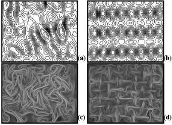
Figure 1: Streamlines computed from measured velocity fields at Re=56 and path length p=2.5 for (a) disordered and (b) ordered magnet array configurations. The ordered case shows clear lines of mirror symmetry. Corresponding stretching fields for (c) disordered and (d) ordered flows, showing the magnitude of stretching over an interval $\Delta$t= 1 period. Regions of strong stretching are localized in both cases.

The experimental configuration, described in more detail elsewhere Voth et al. (2003), is a thin fluid layer (1 mm thick) containing the reactants, that overlies a somewhat deeper conducting fluid layer (3 mm thick). Chaotic flows are created by magneto-hydrodynamic forcing of the conducting fluid layer. A time-periodic electric current (with frequency f in the range 10-140 mHz) passing through the lower layer, in the presence of an array of magnets, drives a time-dependent vortex flow that may be either spatially ordered or disordered depending on the magnet arrangement. The fluid is a 20% glycerol-water mixture (viscosity = 1.74 cP, density = 1.1 g/cm³), about 10 cm x 10 cm in size, but only the central 8 x 8 cm is imaged. The flow in the upper layer is nearly two-dimensional Paret et al. (1997) and typical RMS velocities (U) are 0.05 to 0.7 cm/s. The Reynolds number, Re= $\rho$LU/$\mu$, based on the mean magnet spacing (L=2 cm) is in the range 5 to 75. The path length parameter, p=U/Lf, which describes the mean displacement of a typical fluid element in one forcing period, is in the range 0.5 to 3.5.

We investigate reactive mixing using an aqueous acid-base reaction NaOH + HCl $\rightarrow$ NaCl + H₂O, or H³O+ + OH^- $\rightarrow$ 2H₂O, in the upper fluid layer. We write it schematically as A + B $\rightarrow$ 2P. The reaction is fast and second order. Its rate constant is k=1.1 x 10⁸ M^-1 s^-1, and the reaction speed is characterized by the Damköler number Da= kC₀L²/D, based on the ratio of the diffusion time scale (L²/D) to the reaction time scale (kC₀). Here, the diffusion constant D of either acid or base with its counter-ion is about 10^-5 cm²/s, and C₀=2.2 x10^-2 M is the initial reactant concentration. We note that Da is large ($>$ 10⁵), so that the reaction is limited by the diffusion fluxes toward the lines of contact. However, diffusion is enhanced by the stretching of interfaces. The relative importance of stretching and diffusion is given by the (Lagrangian) Peclet number Pe=L²$\overline{\lambda}$/D, where $\overline{\lambda}$ is the mean Lyapunov exponent of the flow. Here, Pe is typically large and in the range 3.48 x 10⁵ to 1.02 x10⁷.

To determine fluid stretching, we first obtain high resolution velocity fields using particle tracking methods described elsewhere Voth et al. (2002). Streamlines of the measured velocity fields for both ordered and disordered magnet array configurations at Re=56 (and p=2.5) are shown in Figs. 1(a,b), respectively. The disordered flow has no spatial symmetry while the ordered flow has reflection and discrete translation symmetry along the coordinate axes. Regular (non-mixing) regions are found in the ordered flow at a given Re, and in the disordered flow at low Re.

Next, we use the velocity fields to construct displacement maps over a selected time interval $\Delta$t, and then compute stretching fields from the maps by differentiation [15]. This method, originally developed in numerical studies, provides high resolution stretching fields Haller and Yuan (2000); Haller (2001). Examples are shown in Fig. 1(c,d). The local stretching (S) measures the deformation of an infinitesimal circular fluid element located initially at (x,y) over the interval $\Delta$t. The local finite time Lyapunov exponent is defined as $\overline{\lambda}$=(log S)/$\Delta$t. Stretching fields computed over 1 period, corresponding to the disordered and ordered array at Re=56 (p=2.5), are shown in Figs. 1(c,d), respectively. Both fields show a wide distribution of stretching values Arratia and Gollub (2005) stronger at some locations than at others by a factor of 1000. In the ordered case (Fig 1d), it is clear that the stretching is highly inhomogeneous, being much larger along lines passing through stagnation (hyperbolic) points of the flow than in other regions. The strongest overall stretching occurs for the disordered array (Fig. 1c), due in part to the lack of spatial symmetry of the velocity field. We also find stronger stretching for flows with larger p at a given Re and magnet array configuration. The mean Lyapunov exponent $\overline{\lambda}$ is computed by averaging the local values over the image domain.

We now show in Fig. 2 the reaction of initially segregated aqueous solutions containing reactant A (acid) and reactant B (base) at Re=37 and Re=56 for the disordered flow, and also at Re=56 for the ordered flow. Initially, a solid barrier (the dotted line in Fig. 2a) separates the acid, which contains a pH sensitive fluorescent dye, from the base. The barrier is lifted and the reaction is observed over varying numbers N of cycles. (N=10 and N=30 are shown in the upper and lower rows of Fig. 2.)

We define normalized concentration fields for the acid A, base B, and product P, as follows: $\widetilde{A}$=A/A₀, $\widetilde{B}$=B/B₀, and $\widetilde{P}$=P/P_final, where A₀ and B₀ are the initial reactant concentrations, and P_final is the product concentration in the fully reacted state. Using separate calibration experiments, we determine $\widetilde{A}$$(x,y,t)$ from the local light intensity. From the conservation of material expressed in the statement A + B $\rightarrow$ 2P, it can be shown that averaged over the entire cell $\langle\widetilde{P}\rangle$=1-2$\langle\widetilde{A}\rangle$, where $\langle A\rangle$=1/n$\sum_{j=1}^{n}A_{j}$, and n is the number of pixels in the image. Though this relation is not accurate locally due to advection and diffusion, we use $\widetilde{P}$=1-2$\widetilde{A}$ as an approximation to display the local normalized product concentration field.

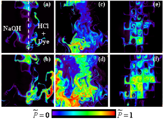
Figure 2: (Color online) Normalized product concentration fields ($\widetilde{P}$) vs. number of periods (N) at p=2.5. (a) Re=37 (disordered), N=10; (b) Same as (a) for N=30; (c) Re=56 (disordered), N=10; (d) Same as (c) for N=30; (e) Re=56 (ordered), N=10; (f) Same as (e) for N=30. Fully reacted regions appear in red, as shown in the color bar. Unreacted regions are shown in black.

As time evolves, the interplay of stretching, diffusion, and reaction creates a complex pattern, with regions of high (red) and low (dark) normalized product concentration. The development of convoluted interfaces is evident early. At longer times, systematic differences between the different flows become clear. For Re=37 (disordered array), the reacted regions are spatially extended, but large unreacted regions remain even after 30 periods. This flow departs less from time-reversibility, a necessary condition for mixing Voth et al. (2003), due to its lower inertia than does the Re=56 case. Even in the reacted regions, the product concentration is small at lower Re.

Product formation is also affected by the extent of regular (non-mixing) islands, which are favored by the mirror symmetry of the ordered flow (Fig. 2e,f), but that also occur for the disordered flow at the lower Re (Fig. 2a,b). These are regions of low stretching where the interface between reactants grows approximately linearly in time, and the local reaction rate is less than in regions of high stretching. Such isolated regions are not visible at in Fig. 2(c,d) (higher Re=56, disordered flow), where the accumulated product is higher than it is in the ordered flow for the same Re and reaction time. These qualitative differences show that the product distribution is substantially affected by the flow pattern.

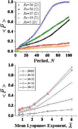
Figure 3: (Color online) (a) Spatial averaged normalized product concentration $\langle\widetilde{P}\rangle$ as a function of time (or N) and Re for several different flows (D=disordered, O=ordered, all at p=2.5). (b) $\langle\widetilde{P}\rangle$ vs. mean Lyapunov exponent ( $\overline{\lambda}$) for various N (disordered flows for various Re). Lines are added to guide the eye. Product growth is slow for small but accelerates for large at later times.

Next we explore the evolution of the spatial average of the normalized product $\langle\widetilde{P}\rangle$ (or the total quantity of product) as a function of time for flows having different dynamical features. Fig. 3(a) shows that the high Re and p disordered flow produces the fastest product growth, while lower Re, p or spatial order substantially reduces the growth rate. The reason is that irreversibility due to inertia (large Re), large particle displacement (p), and the absence of barriers to transport (disorder) are required for rapid mixing. For all flows, the initial product growth is roughly linear rather than exponential in time. This is especially clear for low Re and ordered flows, where there are substantial low stretching regions. Although the simplest theories suggest exponential early growth Chertkov and Lebedev (2003) this is not apparent in the data, most likely due to the wide distribution of local stretching rates first pointed out in Ref. Voth et al. (2002). A numerical study in 2D flows Muzzio and Liu (1996) also finds that non-chaotic regions lead to sub-exponential initial product growth.

The average normalized product $\langle\widetilde{P}\rangle$ is most usefully parameterized by the mean Lyapunov exponent $\overline{\lambda}$ rather than Re or p. In Fig. 3(b), we show the variation of $\langle\widetilde{P}\rangle$ as a function of $\overline{\lambda}$ at different numbers of periods N for disordered flows with different Re (p=2.5). The growth with $\overline{\lambda}$ is approximately linear for small $\overline{\lambda}$ but accelerates for large $\overline{\lambda}$ at the later times.

Although the concentration patterns are complex, the evolution of $\langle\widetilde{P}\rangle$ (at least after an initial transient) turns out to be a function only of N and $\overline{\lambda}$. In Fig. 4, we plot $\langle\widetilde{P}\rangle$ vs. $\overline{\lambda}N$ for the disordered flows at various Re and p. We find that product concentration curves collapse onto a single master curve with no adjustable parameters. This is a surprising result because even though the flows have the same magnet array configuration, they possess different degrees of time reversibility and mean particle displacements per cycle, and regular regions occur to a different extent in the various flows. In the insert to Fig. 4, we show that this scaling behavior can be extended to ordered flows as well. Remarkably, the rescaled ordered flow data for different Re fall onto the same master curve as the disordered array cases, which include various Re and p.

The dependence of product concentration on and time has been recently considered theoretically K rolyi and Tel (2005) using a simplified model for the reaction interface. The authors suggest that after a short time (t$<$1/$\overline{\lambda}$) the normalized concentration should be described by

$$\langle\widetilde{P}\rangle=1-exp({-a{\overline{\lambda}}N})$$ (1)

where a is a constant. A similar relationship is also found in a numerical study using periodic boundary conditions for 2D flows Giona et al. (2002a). This result, shown by the dotted line in Fig. 4 for the best fitting value of a describes our data adequately for $\emph{$\overline{\lambda}N$}<300$. However, for larger values, $\langle\widetilde{P}\rangle$ grows more rapidly than this form predicts.

Other theoretical works show a double exponential growth, or a more complex spatio-temporal behavior depending on the reaction rate Sokolov and Blumen (1991a); Tang and Boozer (1996) or the presence of boundaries Chertkov and Lebedev (2003). Finally, one might consider a solution of Floquet form consisting of a sum of several exponentials Liu and Haller (2004), since the flow is periodically driven. However, none of these forms is found to fit the data over the entire range of $\overline{\lambda}N$.

We can fit the entire data set (ordered, disordered, and different Re and p) to a single empirical function of the form $\langle\widetilde{P}\rangle=1-exp[-\alpha\overline{\lambda}N-\beta(\overline{\lambda}N)^{2}]$, where $\alpha$=0.0018 $\pm$ 1.9 x 10^-4 and $\beta$= 6.2 x 10^-6 $\pm$ 2.5 x 10^-7 are constants. (However, the constants and could depend on the initial shape of the reaction interface, a variable we did not explore.) Note that this equation (solid line in Fig. 4) fits the data over the entire range reasonably well. For the lower values of $\overline{\lambda}N$, the quadratic dependence is weak and we recover Eq.(1). The more rapid approach to saturation at late times might be due to the transport of initially segregated reactants to regions where they can react. A similar transport effect was demonstrated by Voth et al. Voth et al. (2003) for passive mixing. Note that we cannot reach the fully reacted state for $\emph{$\overline{\lambda}$}<3$.

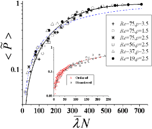
Figure 4: (Color online) Dependence of $\langle\widetilde{P}\rangle$ on the product of the mean Lyapunov exponent ($\overline{\lambda}$) and period N for disordered flows at various Re and p. Insert: Early behavior for both ordered and disordered flows (at various Re and p). The dotted and solid lines correspond to Eq.1 (a=0.00263) and the empirical fit described in the text, respectively.

In conclusion, we study the interplay of stretching, diffusion, and fast reaction experimentally, with direct measurement of the stretching fields. The strong spatial heterogeneity of stretching, with a distribution spanning many decades, Voth et al. (2002); Arratia and Gollub (2005) causes the early product growth to deviate strongly from the exponential behavior expected for uniform stretching. Spatial symmetry, particle displacement, and the departure from time reversibility affect the reaction progress (and $\overline{\lambda}$). However, the normalized product concentration up to the fully reacted state approximately follows a single master curve with $\overline{\lambda}N$ as the independent variable, where $\overline{\lambda}$ is the measured mean Lyapunov exponent and N is the number of mixing cycles. This result allows quantitative prediction of the total product as a function of time for several chaotically mixing flows with different dynamical features such as spatial symmetry and the extent of departures from reversibility. This scaling is not expected to apply to turbulent flows, but may be appropriate for a variety of fast reactions that are stirred by chaotic advection.