Holographic hessence models

Abstract

We discuss the evolution of holographic hessence model, which satisfies the holographic principle and can naturally realizes the equation of state crossing $-1$. By discussing the evolution of the models in the $w-w^{\prime}$ plane, we find that, if $c\geq 1$, $w_{he}\geq-1$ and $\dot{V}<0$ keep for all time, which are quintessence-like. However, if $c<-1$, which mildly favors the current observations, $w_{he}$ evolves from $w_{he}>-1$ to $w_{he}<-1$, and the potential is a nonmonotonic function. In the earlier time, the potential must be rolled down, and then be climbed up. Considered the current constraint on the parameter $c$, we reconstruct the potential of the holographic hessence model.

PACS numbers: 98.80.-k, 98.80.Es, 04.30.-w, 04.62.+v

e-mail: wzhao7@mail.ustc.edu.cn

1 Introduction

Numerous and complementary cosmological observations indicate that the expansion of the universe is undergoing cosmic acceleration at the present time[1]. This cosmic acceleration is viewed as due to a mysterious dominant component, dark energy, with negative pressure. The combined analysis of cosmological observations suggests that the universe is spatially flat, and consists of about $70\%$ dark energy, $30\%$ dust matter (cold dark matter plus baryons), and negligible radiation. Although we can affirm that the ultimate fate of the universe is determined by the feature of dark energy, the nature of dark energy as well as its cosmological origin remain enigmatic at present. Explanations have been sought within a wide range of physical phenomena, including a cosmological constant, exotic fields[2, 3, 4, 5, 6], a new form of the gravitational equation[7], etc. Recently, a new model stimulated by the holographic principle has been put forward to explain the dark energy[8, 9]. According to the holographic principle, the number of degrees of freedom of a physical system scales with the area of its boundary. In the context, Cohen et al[10] suggested that in quantum field theory a short distant cutoff is related to a long distant cufoff due to the limit set by formation of a black hole, which results in an upper bound on zero-point energy density. In line with this suggest, Hsu and Li[8, 9] argued that this energy density could be views as the holographic dark energy satisfying

$$\rho_{de}=3c^{2}M_{P}^{2}L^{-2}~{},$$ (1)

where $c$ is a numerical constant, and $M_{P}\equiv 1/\sqrt{8\pi G}$ is the reduced Planck mass. If we take $L$ as the size of the current universe, for instance the Hubble scale $H^{-1}$, then the dark energy density will be close to the observed data. However, Hsu[8] pointed out that this yields a wrong equation of state for dark energy. Li[9] subsequently proposed that the IR cut-off $L$ should be taken as the size of the future event horizon

$$L=R_{eh}(a)=a\int_{t}^{\infty}{d\tilde{t}\over a(\tilde{t})}=a\int_{a}^{\infty}{d\tilde{a}\over H\tilde{a}^{2}}~{}.$$ (2)

Then the problem can be solved nicely and the holographic dark energy model can thus be constructed successfully. The holographic dark energy scenario may provide simultaneously natural solutions to both dark energy problems as demonstrated in Ref.[9]. The only undetermined parameter $c$ should be fixed by the observations. If $c\leq 1$, which satisfies the original bound $L^{3}\rho_{de}\leq LM_{p}^{2}$, the equation of state (EOS) of dark energy evolves from the state of $w>-1$ to $w<-1$, and the critical state of $w=-1$ must be crossed. If $c>1$, the EOS of dark energy keeps $w>-1$[9], which naturally avoided the cosmic big rip. However, the original bound $L^{3}\rho_{de}\leq LM_{p}^{2}$ will be violated. Since the model we discuss here is only a phenomenological framework and it is unclear whether it is appropriate to tightly constrain the value of $c$ by means of the analogue to the black hole. As a matter of fact, the possibility of $c>1$ has been seriously dealt with and a modest value of $c$ larger than one could be favored in the literature[11]. In this paper, we consider the general case with $c$ as a free parameter.

For a kind of realized dark energy model, the feature of EOS crossing $-1$ can not be realized by the simple quintessence, phantom, or k-essence[12]. The quintom is one of the simplest models with EOS crossing $-1$, which is the combination of a quintessence $\phi_{1}$ and a phantom $\phi_{2}$. The hessence is a kind of simple quintom[13, 14], which has the lagrangian density

$${\cal L}_{he}=\frac{1}{2}(\partial_{\mu}\phi_{1})^{2}-\frac{1}{2}(\partial_{\mu}\phi_{2})^{2}-V(\phi_{1}^{2}-\phi_{2}^{2})~{},$$ (3)

where the potential function $V(\phi_{1}^{2}-\phi_{2}^{2})$ is free for the models. Different choice of $V$ follows a different evolution of the universe. In Ref.[15], the authors found that this kind of models may be the local effective approximation of the D3-brane Universe. In Ref.[14], we have proved that the evolution of potential function can be exactly determined by the EOS of hessence $w_{he}(z)$ and its evolution $w_{he}^{\prime}(z)$. If considered the holographic constraint in Eq.(1), the EOS of the hessence can be exactly determined for a fixed $c$. So the potential function for the holographic hessence only depends on the parameter $c$. In this letter, we first discuss the evolution of the EOS and potential of the holographic hessence models for the different $c$. Then considered the constraint on $c$ from the current observations, we reconstruct the potential function of holographic hessence models.

2 Holographic hessence models

We consider the action

$$S=\int d^{4}x\sqrt{-g}\left(-\frac{\cal R}{16\pi G}+{\cal L}_{he}+{\cal L}_{m}\right),$$ (4)

where $g$ is the determinant of the metric $g_{\mu\nu}$, $\cal R$ is the Ricci scalar, ${\cal L}_{he}$ and ${\cal L}_{m}$ are the lagrangian densities of the hessence dark energy and matter, respectively. The lagrangian density of hessence is in Eq.(3). One can easily find that this lagrangian is invariant under the transformation

$$\phi_{1}\rightarrow\phi_{1}\cosh(i\alpha)-\phi_{2}\sinh(i\alpha)~{},$$ (5)

$$\phi_{2}\rightarrow-\phi_{1}\sinh(i\alpha)+\phi_{2}\cosh(i\alpha)~{},$$ (6)

where $\alpha$ is constant. This property makes one can rewrite the lagrangian density (3) in another form

$${\cal L}_{he}=\frac{1}{2}\left[(\partial_{\mu}\phi)^{2}-\phi^{2}(\partial_{\mu}\theta)^{2}\right]-V(\phi)~{},$$ (7)

where we have introduced two new variables $(\phi,~{}\theta)$, i.e.

$$\phi_{1}=\phi\cosh\theta~{},~{}~{}~{}~{}~{}~{}\phi_{2}=\phi\sinh\theta~{}.$$ (8)

Consider a spatially flat FRW (Friedmann-Robertson-Walker) universe with metric

$$ds^{2}=dt^{2}-a^{2}(t)\gamma_{ij}dx^{i}dx^{j}~{},$$ (9)

where $a(t)$ is the scale factor, and $\gamma_{ij}=\delta^{i}_{j}$ denotes the flat background space. Assuming $\phi$ and $\theta$ are homogeneous, from the action in (4), we obtain the equations of motion for $\phi$ and $\theta$

$$\ddot{\phi}+3H\dot{\phi}+\phi\dot{\theta}^{2}+dV/d\phi=0~{},$$ (10)

$$\phi^{2}\ddot{\theta}+(2\phi\dot{\phi}+3H\phi^{2})\dot{\theta}=0~{},$$ (11)

where $H\equiv\dot{a}/a$ is the Hubble parameter, an overdot denotes the derivatives with respect to cosmic time. Eq.(11) implies

$$Q=a^{3}\phi^{2}\dot{\theta}={\rm const}~{},$$ (12)

which is associated with the total conserved charge within the physical volume due to the internal symmetry[13]. This relation turns out

$$\dot{\theta}=\frac{Q}{a^{3}\phi^{2}}~{}.$$ (13)

Substituting this into Eq.(10), we can rewrite the kinetic equation as

$$\ddot{\phi}+3H\dot{\phi}+\frac{Q^{2}}{a^{6}\phi^{3}}+\frac{dV}{d\phi}=0~{},$$ (14)

which is equivalent to the energy conservation equation of the hessence $\dot{\rho}_{he}+3H(\rho_{he}+p_{he})=0$. The pressure, energy density and the EOS of the hessence are

$$p_{he}=\frac{1}{2}\dot{\phi}^{2}-\frac{Q^{2}}{2a^{6}\phi^{2}}-V(\phi)~{},~{}~{}~{}~{}~{}~{}~{}\rho_{he}=\frac{1}{2}\dot{\phi}^{2}-\frac{Q^{2}}{2a^{6}\phi^{2}}+V(\phi)~{},$$ (15)

$$w_{he}=\left.\left[\frac{1}{2}\dot{\phi}^{2}-\frac{Q^{2}}{2a^{6}\phi^{2}}-V(\phi)\right]\right/\left[\frac{1}{2}\dot{\phi}^{2}-\frac{Q^{2}}{2a^{6}\phi^{2}}+V(\phi)\right]~{},$$ (16)

respectively. It is easily seen that $w_{he}\geq-1$ when $\dot{\phi^{2}}\geq Q^{2}/(a^{6}\phi^{2})$, while $\omega_{he}\leq-1$ when $\dot{\phi^{2}}\leq Q^{2}/(a^{6}\phi^{2})$. The transition occurs when $\dot{\phi^{2}}=Q^{2}/(a^{6}\phi^{2})$. In the case of $Q\equiv 0$, the hessence becomes the quintessence model. From the expression of EOS of hessence, we can find it is only dependant of the potential function $V(\phi)$. If $V(\phi)$ is determined, $w$ is also determined. On the contrary, if $w(z)$ is fixed, the potential function $V(\phi)$ also can be solved. Here we consider the holographic hessence models, which satisfies the holographic constraint in Eq.(1). Consider now a spatially flat FRW universe with matter component $\rho_{m}$ (including both baryon matter and cold dark matter) and holographic hessence component $\rho_{he}$. The Friedmann equation reads

$$3H^{2}M_{p}^{2}=\rho_{m}+\rho_{he}~{},$$ (17)

or equivalently,

$${H^{2}\over H_{0}^{2}}=\Omega_{m0}a^{-3}+\Omega_{he}{H^{2}\over H_{0}^{2}}~{}.$$ (18)

Combining the definition of the holographic dark energy (1) and the definition of the future event horizon (2), we derive

$$\int_{a}^{\infty}{d\ln\tilde{a}\over H\tilde{a}}={c\over Ha\sqrt{\Omega_{he}}}~{}.$$ (19)

We notice that the Friedmann equation (18) implies

$${1\over Ha}=\sqrt{a(1-\Omega_{he})}{1\over H_{0}\sqrt{\Omega_{m}^{0}}}~{}.$$ (20)

Substituting (20) into (19), we get easily the dynamics satisfied by the dark energy, i.e. the differential equation about the fractional density of dark energy,

$$\Omega^{\prime}_{he}=\Omega_{he}(1-\Omega_{he})\left(1+{2\over c}\sqrt{\Omega_{he}}\right),$$ (21)

where the prime denotes the derivative with respect to $\ln a$. This equation describes behavior of the holographic dark energy completely, and it can be solved exactly. It is easy to prove that, this equation has only one steady attractor solution

$$\Omega_{he}=1.$$ (22)

In the solution, the hessence is dominant in the universe, and the component of matter is negligible.

Important observables to reveal the nature of dark energy are the EoS $w$ and its time derivative in units of Hubble time $w^{\prime}$. The SNAP mission is expected to observe about $2000$ SNIa each year, over a period of three years. Most of these SNIa are at the redshift $z\in[0.2,~{}1.2]$. The SNIa plus weak lensing methods conjoined can determine the present equation of state ratio, $\omega_{0}$, to $5\%$, and its time variation, $\omega^{\prime}$, to $0.11$ [16]. It has a powerful ability to differentiate the various dark energy models. From the energy conservation equation of the holographic hessence, the EOS of the dark energy can be given [9]

$$w_{he}=-1-{1\over 3}{d\ln\rho_{he}\over d\ln a}=-{1\over 3}\left(1+{2\over c}\sqrt{\Omega_{he}}\right)~{},$$ (23)

and its evolution is

$$w_{he}^{\prime}=-\frac{\sqrt{\Omega_{he}}}{3}(1-\Omega_{he})\left(1+\frac{2}{c}\sqrt{\Omega_{he}}\right).$$ (24)

It can be seen clearly that the equation of state of the holographic dark energy evolves dynamically and satisfies $-(1+2/c)/3\leq w_{he}\leq-1/3$ due to $0\leq\Omega_{he}\leq 1$. The parameter $c$ plays a significant role in this model. If one takes $c=1$, the behavior of the holographic dark energy will be more and more like a cosmological constant with the expansion of the universe, such that ultimately the universe will enter the de Sitter phase in the far future. As is shown in[9], if one puts the parameter $\Omega_{he0}=0.73$ into (23), then a definite prediction of this model, $w_{he0}=-0.903$, will be given. On the other hand, if $c<1$, the holographic dark energy will exhibit appealing behavior that the equation of state crosses the “cosmological-constant boundary” (or “phantom divide”) $w=-1$ during the evolution. This kind of dark energy is referred to as “quintom” [5] which is slightly favored by current observations [17]. If $c>1$, the equation of state of dark energy will be always larger than $-1$ such that the universe avoids entering the de Sitter phase and the Big Rip phase. Hence, we see explicitly, the value of $c$ is very important for the holographic dark energy model, which determines the feature of the holographic hessence as well as the ultimate fate of the universe.

Now, we discuss the dark energy models in the $w-w^{\prime}$ plane, which clearly shows the evolution character of the dark energy. The simplest model, cosmological constant, has the effective state of $w=-1$ and $w^{\prime}=0$, which corresponds to a fixed point in the $w-w^{\prime}$ plane. Generally, the dynamics model of dark energy shows a line in this plane, which describes the evolution of its EOS[18]. The simple quintessence has the state of $w\geq-1$, which only occupies the region of $w^{\prime}>-3(1+w)(1-w)$. The phantom field ($w\leq-1$) occupies the region of $w^{\prime}<-3(1+w)(1-w)$. The evolution of hessence in the $w-w^{\prime}$ plane is discussed in Ref.[14]. Here we brief it as below. From the kinetic equation (14), one can get

$$1+\frac{1}{6}\frac{d\ln x}{d\ln a}=-\frac{1}{3HV}\frac{\dot{V}}{1+w_{he}}~{},$$ (25)

where $a$ is the scale factor, and we have set the present scalar factor $a_{0}=1$. The function $x$ is defined by

$$x\equiv\left|\frac{1+w_{he}}{1-w_{he}}\right|=\left|\frac{\frac{1}{2}\dot{\phi}^{2}-\frac{Q^{2}}{2a^{6}\phi^{2}}}{V}\right|~{},$$ (26)

and

$$\frac{d\ln x}{d\ln a}=\frac{2w_{he}^{\prime}}{(1+w_{he})(1-w_{he})}~{}.$$ (27)

This equation can be rewritten as

$$\left.\left(1+\frac{w_{he}^{\prime}}{3(1+w_{he})(1-w_{he})}\right)\right/\left(\frac{2\dot{V}}{3H(1+w_{he})\rho_{he}}\right)=-\frac{\rho_{he}}{2V}<0~{}.$$ (28)

which follows that

$$F\dot{V}<0,$$ (29)

where we have defined $F\equiv w_{he}^{\prime}+3(1+w_{he})(1-w_{he})$. So the $w-w^{\prime}$ plane is divided into four parts

I:       $F>0$   &   $w>-1$;       II:       $F>0$   &   $w<-1$;

III:       $F<0$   &   $w<-1$;      IV:       $F<0$   &   $w>-1$.
This can be seen clearly in Figure 1. From Eq. (29), one can easily find that $\dot{V}<0$ is satisfied in Region I and II (rolling-down region), the field rolling down the potential, and $\dot{V}>0$ is satisfied in Region III and IV (climbing-up region), the field climbing up the potential. So from the value of the function $w^{\prime}+3(1-w)(1+w)$ being positive or negative, one can immediately judge how the field evolves at that time. Toward the holographic hessence models, from the equations (23) and (24), we have

$$F=\frac{1}{3}\left(\frac{2}{c}\Omega_{he}^{2}+\Omega_{he}^{\frac{3}{2}}-\frac{4+2c}{c^{2}}\Omega_{he}-\frac{c+4}{c}\sqrt{\Omega_{he}}+8\right).$$ (30)

For a fixed $c$, $F$ only depends on the value of $\Omega_{he}$. So the evolution of potential function of hessence is also exactly determined by the evolution of $\Omega_{he}$. It is easily to find that this is a monotonic increasing function with the increasing $\Omega_{he}$. In order to exactly determine this function, one must numerically solve the Eq.(21) and get function $\Omega_{he}(z)$. Here we only concern on that whether the potential function of holographic hessence is monotonic. If $F<0$ is holden for all time, the potential is a monotonic increasing function. But it is not same with the phantom models, since the cosmological constant can be crossed in the this hessence. If $F>0$ is holden for all time, the potential is a monotonic decreasing function. Since $w=-1$ also can be crossed in this case, the models are different from the simple quintessence. If the state of $F=0$ is crossed in the evolution of hessence, the potential function of hessence can not be a monotonic function.

Here we focus on the initial and finial states of the holographic hessence, and investigate them in the $w-w^{\prime}$ plane. In the initial condition with $\Omega_{he}\rightarrow 0$, one has

$$(w_{he},w_{he}^{\prime})\rightarrow\left(-\frac{1}{3},~{}0\right),$$ (31)

$$F=w_{he}^{\prime}+3(1+w_{he})(1-w_{he})\rightarrow\frac{8}{3}>0,$$ (32)

which is in the rolling-down region (Region I), and independent of value of $c$. So in any case of models, they evolve from the region I, which is quintessence-like. However, in the finial stage with $\Omega_{he}\rightarrow 1$, one has

$$w_{he}\rightarrow-{1\over 3}\left(1+{2\over c}\right),~{}~{}~{}~{}w_{he}^{\prime}\rightarrow 0,$$ (33)

and

$$F=\frac{4}{3}\left(2-\frac{1}{c}-\frac{1}{c^{2}}\right).$$ (34)

For the different choice of $c$, the finial value of $F$ is different.

$$c > 1,~{}~{}F>0~{}~{}~{}(~{}\rm in~{}~{}the~{}~{}rolling-down~{}~{}region~{}),$$ (35)

$$c = 1,~{}~{}F=0~{}~{}~{}(~{}\rm at~{}~{}the~{}~{}critical~{}~{}point~{}),$$ (36)

$$c < 1,~{}~{}F<0~{}~{}~{}(~{}\rm in~{}~{}the~{}~{}climbing-up~{}~{}region~{}).$$ (37)

In Figure 1, we have plotted the evolution of three different holographic hessence models with $c=1.5,1.0,0.5$, respectively, where the arrows indicate the evolution direction of hessence with the increasing value of $\Omega_{he}$ from $\Omega_{he}=0$ to $\Omega_{he}=1$. From this figure, we can find that, if $c>1$ is chosen, which violates the holographic constraint, the hessence is in the Region I (rolling-down region) for all time, so the potential of hessence is a monotonic damping function, which is similar the quintessence models. This is consistent to the previous conclusion that holographic dark energy with $c>1$ can be described by the quintessence fields. However, if the fixed $c$ is smaller than $1$, which satisfies the holographic constraint, the hessence must evolve from Region I (rolling-down region) to Region IV (climbing-up region), and finally to Region III (climbing-up region). So the potential of hessence is not a monotonic function. The field $\phi$ rolls down the potential at earlier stage, and later it turns to climb up. With the expansion of the universe, the state of $F=0$ must be crossed. The EOS of hessence also turns from the region of $w>-1$ to that of $w<-1$, and the state of $w=-1$ must be crossed. So dark energy is quintom-like. We note that the time of $F=0$ is a little earlier than that of $w=-1$. If $c=1$ is chosen, the holographic hessence is also in Region I for all time, and finally it turns to the critical state of $(w,w^{\prime})=(-1,0)$ with the expansion of the universe, and the universe is an exact de Sitter expansion.

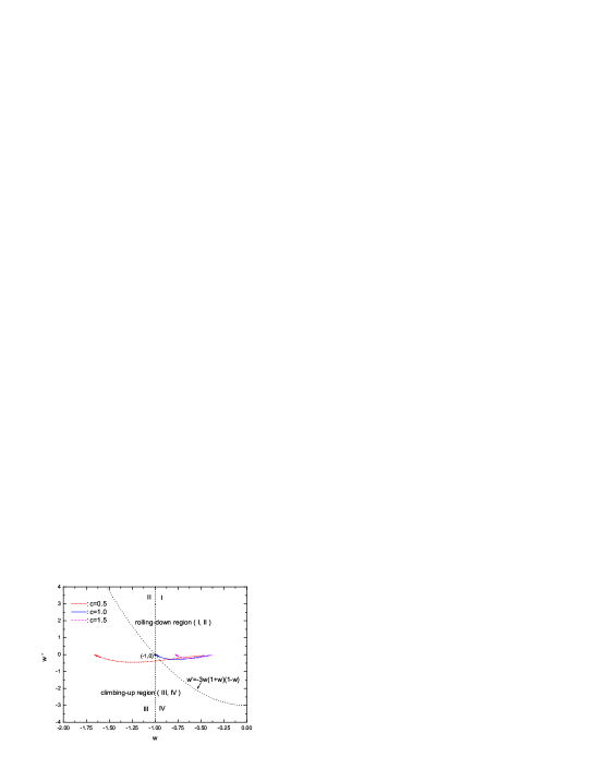
Figure 1: The holographic hessence models evolve in the $w-w^{\prime}$ plane, where we have considered three models with $c=0.5,1.0,1.5$, respectively. The arrows denote the evolution direction of the models with the expansion of the universe.

3 Reconstruct the holographic hessence models

From the previous discussion, we find the value of the parameter $c$ should be fixed by the cosmological observations. This has been discussed by a number of authors[17]. In the recent work[19], the authors have constrained the holographic dark energy by the current observations of SNIa (Type Ia Supernova), CMB (cosmic microwave background radiation), and BAO (baryon acoustic oscillation). If setting $c$, $\Omega_{m0}$ and $H_{0}$ as the free parameters, and only using the up-to-date gold sample of SNIa consisted of $182$ data[20], the author found that the best-fit for the analysis of gold sample of SNIa happens at

$$c=0.37,~{}~{}\Omega_{m0}=0.43,~{}~{}h=0.64.$$ (38)

By choosing $h=0.64$, the $1\sigma$ fit values for the parameters are:

$$c=0.37^{+0.56}_{-0.21},~{}~{}\Omega_{m0}=0.43^{+0.08}_{-0.14}.$$ (39)

It is obvious that the SNIa data alone seem not sufficient to constrain the holographic dark energy models strictly. The confidence region of $c$ is very large, and the best fit of $\Omega_{m0}$ is evidently different from other constraint[21]. In the previous work[25], the authors found that the holographic dark energy model is very sensitive to the value of the present Hubble parameter $h$. So it is very important to use other results of CMB and LSS (large-scale structure), which are observational quantities irrelevant to $h$ as a complement to SNIa data. The authors considered the recent observations on the CMB shift parameter $R=1.70\pm 0.03$[22] and the measurement of BAO peak in the distribution of SDSS luminous red galaxies[23]. From the constraints of the combination of SNIa, CMB and BAO, and considered the prior $h=0.72\pm 0.08$, which is got from the Hubble Space Telescope Key Project (HST)[24], the fit values for model parameters with $1-\sigma$ errors are

$$c=0.91^{+0.23}_{-0.19},~{}~{}\Omega_{m0}=0.29\pm 0.03.$$ (40)

It is clear that in the joint analysis the derive value for matter density $\Omega_{m0}$ is very reasonable, which is important for this model is the determination of the value of $c$.

As shown in [25] and the discussion above, the constraint of $h$ can evidently change the constraint result. In order to show how strongly biased constraints can be derived from a factitious prior on $h$, the author also considered a strong $HST$ prior, fixing $h=0.72$. The constraint in equation (40) becomes

$$c=0.42\pm 0.05,~{}~{}\Omega_{m0}=0.24^{+0.02}_{-0.03}.$$ (41)

We find that the confidence level contours get very evident shrinkage and left-shift in the $c-\Omega_{m0}$ parameter-plane, which also changes the evolution of the EOS parameter of the dark energy and deceleration parameter of the universe[19]. These all exactly consist with the previous results[25]. We also find that the constraint of $c$ in (40) and (41) are not overlapped, which is because that the confidence level in these results are two low. If considered the fit values for model parameters with $3-\sigma$ errors, the conclusion will be much improved[19, 25].

However, if setting the Hubble constant as a free parameter in the range of $(0.64,0.80)$, the constraint becomes

$$c=0.82^{+0.11}_{-0.13},~{}~{}\Omega_{m0}=0.28^{+0.03}_{-0.02}.$$ (42)

which also have shrinkage and left-shift in the $c-\Omega_{m0}$ plane, comparing with the results in (40).

From these joint analysis, we can find that, though the possibility of $c>1$ can not be excluded in one-sigma error range, the possibility of $c<1$ is much more favored, which determined that the dark energy is quintom-like, and the EOS crosses $-1$ at some time.

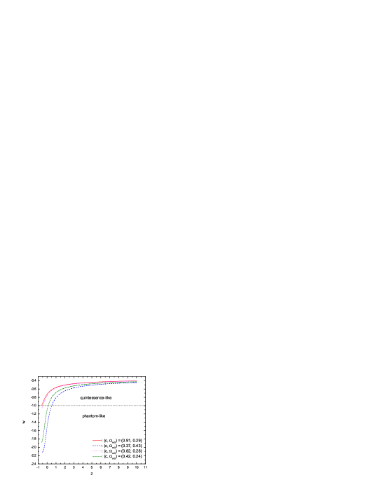
Figure 2: From the observations, we solve the EOSs of the holographic hessence models.

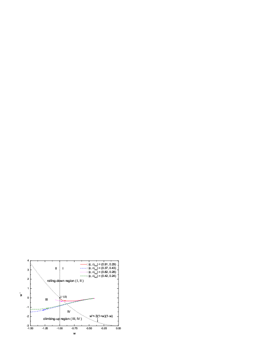
Figure 3: The reconstructed holographic hessence models evolve in the $w-w^{\prime}$ plane, where the arrows denote the evolution direction of the models with the expansion of the universe.

From the differential equation (21), we can get the evolution equation of $\Omega_{he}$ with the redshift $z$

$$\frac{d\Omega_{he}}{dz}=-(1+z)^{-1}\Omega_{he}(1-\Omega_{he})\left(1+{2\over c}\sqrt{\Omega_{he}}\right).$$ (43)

For the determined parameters $c$ and $\Omega_{he0}=1-\Omega_{m0}$, one can numerically solve this equation and get $\Omega_{he}=\Omega_{he}(z)$. Inserting this into equations (23) and (24), we can get the EOS of the holographic hessence $w=w(z)$ and its evolution $w^{\prime}=w^{\prime}(z)$. In Figures 2 and 3 , we have plotted the EOS and its evolution of the holographic hessence with best-fit parameters in the $w-z$ and $w-w^{\prime}$ planes. From Figure 2, we find that, in the earlier stage of universe, the $w>-1$ holds for all cases, and the hessence are quintessence-like. But the values of EOS decrease with time, and they become phantom-like at present time for the case of $c=0.37$ and $c=0.42$. So the cosmological constant has been crossed. In the cases of $c=0.91$ and $0.82$, though $w>-1$ is holden until now, $w<-1$ will occur in the near future, and crossing the cosmological constant is unavoidable. This feature determines that this holographic dark energy can not be described by the quintessence, phantom, k-essence, or Yang-Mills field models[12, 6]. But in the hessence models, it can be naturally and simply realized. From Figure 3, we find that, in the earlier stage, the hessence models are all in Region I (rolling-down region). With the expansion of the universe, these all models will cross the line with $F=0$ and enter into the Region IV, where although $w>-1$ is kept, the hessence fields begin to clime up the potentials. At last, the hessence models all cross the cosmological constant bound and stay in the Region III, where the hessences are phantom-like, and the potentials are climbed up. So the potentials of these holographic hessence are not a monotonic function, which is consistent to the previous discussion.

With these solved EOSs, we can reconstruction the potential of the holographic hessence models. Consider the FRW Universe, which is dominated by the non-relativistic matter and a spatially homogeneous hessence field $\phi$. The energy conservation equation of the hessence field is

$$\dot{\rho}_{he}+3H(\rho_{he}+p_{he})=0~{},$$ (44)

which yields

$$\rho_{he}(z)=\rho_{he0}\exp\left[3\int_{0}^{z}(1+w_{he})d\ln(1+\tilde{z})\right]\equiv\rho_{he0}E(z)~{},$$ (45)

where the subscript $0$ denotes the value of a quantity at the redshift $z=0$ (present). From the expresses of the pressure and energy density of the hessence, we get

$$V(\phi)=\frac{1}{2}\left(1-w_{he}\right)\rho_{he}~{},$$ (46)

$$\dot{\phi}^{2}=\frac{Q^{2}}{a^{6}\phi^{2}}+(1+w_{he})\rho_{he}~{}.$$ (47)

Inserting the formula in these two equations, and after some normal calculation, we get[14]

$$\frac{d\tilde{\phi}}{dz}=\frac{\sqrt{3}}{(1+z)}\left[\frac{C(1+z)^{6}\tilde{\phi}^{-2}+(1+w_{he})E(z)}{r_{0}(1+z)^{3}+E(z)}\right]^{1/2}~{},$$ (48)

$$\tilde{V}[\phi]=\frac{1}{2}(1-w_{he})E(z)~{},$$ (49)

where $r_{0}\equiv\Omega_{m0}/\Omega_{he0}$ is the energy density ratio of matter to hessence at present time, and the dimensionless quantities are defined by

$$\tilde{\phi}\equiv\frac{\phi}{M_{p}}~{},~{}~{}~{}~{}~{}\tilde{V}\equiv\frac{V}{\rho_{he0}}~{},~{}~{}~{}~{}~{}C\equiv\frac{Q^{2}}{\rho_{he0}M_{p}^{2}}~{}.$$ (50)

These two equations relate the hessence potential $V(\phi)$ to the EOS of the hessence $w_{he}(z)$. Given an effective $w_{he}(z)$, the construction Eqs. (48) and (49) allow us to construct the hessence potential $V(\phi)$.

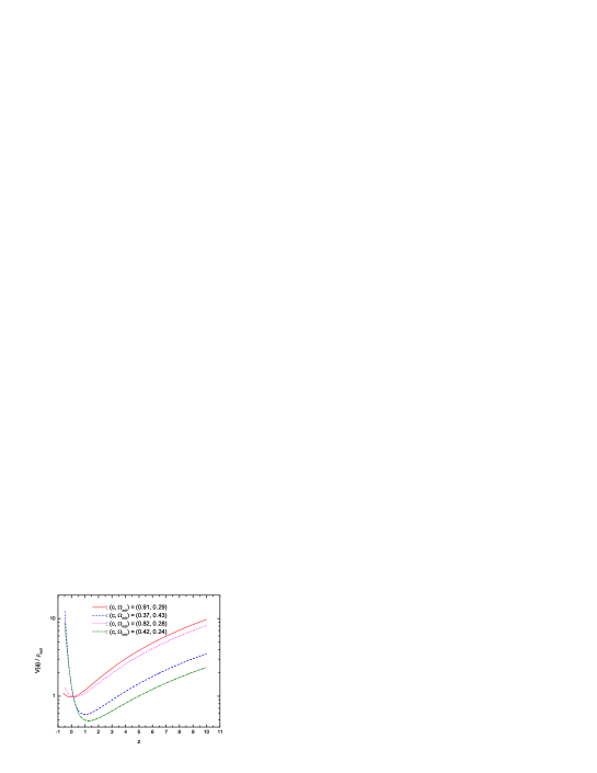
Figure 4: Evolution of potentials of holographic hessence models.

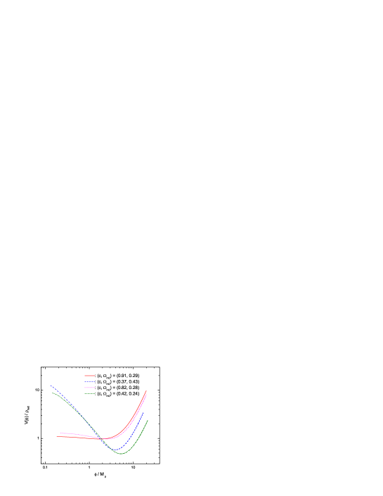
Figure 5: Constructed potentials of holographic hessence models.

Using the solved EOSs of the holographic hessence models in Figure 2, we numerically solve the equations (48) and (49), which are shown in Figures 4 and 5, where we have chosen the initial condition with $C=10.0$ and $\phi_{0}=0.1$. From Figure 4, we find that, for the cases with $c=0.37$ and $c=0.42$, the potentials are decreasing with the expansion of the universe in the earlier stage, which are same with the quintessence models[26]. But after the time, where $z\sim 1$, the potentials begin to increase, and at present time, the potential functions are increasing functions, which are similar to a phantom model. For the cases of $c=0.91$ and $c=0.82$, although the potential functions are monotonically decreasing until the present time, they all will begin to increase with time in the near future. Once again, from Figure 5, we find that these four potentials are all not the monotonic functions, since we have used $c<1$, which is consistent to the previous analysis. The only difference is that the lowest positions of these potentials are different, which is determined by the initial condition and the parameter $c$. These are different from the simple quintessence, k-essence and tachyon models[26].

4 summary

In this letter, we have investigated the hessence models, which satisfy the holographic principle. The potential of the hessence is determined by the holographic principle. We have discussed the evolution of the holographic hessence in the $w-w^{\prime}$ plane, and found that the potential function only depends on the parameter $c$. If $c\geq 1$ is chosen, $w_{he}\geq-1$ is kept for all time, and hessence field $\phi$ rolls down the potential, which is similar to the quintessence models. However if $c<1$ is chosen, which mildly favor the observations, the EOS of the models evolve from the region of $w_{he}>-1$ to that of $w_{he}<-1$, and state of $w_{he}=-1$ must be crossed. The potential of model is not a monotonic function. In the early time, the hessence is quintessence-like, the EOS is $w_{he}>-1$ and $\dot{V}<0$. Then it enters into the region with $w_{he}>-1$ and $\dot{V}>0$, where the potential begins to be climbed up. At last, the model must enter and stay in the phantom-like region with $w_{he}<-1$ and $\dot{V}>0$. Considered the current constraint of the parameter $c$, we have reconstruct the potential of the holographic hessence models, which are all the nonmonotonic functions.

ACKNOWLEDGMENT: The author thanks X.Zhang for helpful discussion.

References

- [1] A.G.Riess et al., Astron.J. 116, 1009 (1998); S.Perlmutter et al., Astrophys.J. 517, 565 (1999); C.L.Bennett et al., Astrophys.J.Suppl. 148, 1 (2003); D.N.Spergel et al., arXiv:astro-ph/0603449; M.Tegmark et al., Astrophys.J. 606, 702 (2004);
- [2] C.Wetterich, Nucl.Phys.B 302, 668 (1988); Astron.Astrophys. 301, 321 (1995); B.Ratra and P.J.E.Peebles, Phys.Rev.D 37, 3406 (1988); R.R.Caldwell, R.Dave and P.J.Steinhardt, Phys.Rev.Lett. 80, 1582 (1998); W.Zhao, arXiv:astro-ph/0604459;
- [3] R.R.Caldwell, Phys.Lett.B 545, 23 (2002); S.M.Carroll, M.Hoffman and M.Trodden, Phys.Rev.D 68, 023509 (2003); R.R.Caldwell, M.Kamionkowski and N.N.Weinberg, Phys.Rev.Lett. 91, 071301 (2003); M.P.Dabrowski, T.Stachowiak and M.Szydlowski, Phys.Rev.D 68, 103519 (2003); V.K.Onemli and R.P.Woodard, Phys.Rev.D 70, 107301 (2004);
- [4] C.Armendariz-Picon, T.Damour and V.Mukhanov, Phys.Lett.B 458, 209 (1999) ; T.Chiba, T.Okabe and M.Yamaguchi, Phys.Rev.D 62, 023511 (2000); C.Armendariz-Picon, V.Mukhanov and P.J.Steinhardt, Phys.Rev.D 63, 103510 (2001); T.Chiba, Phys.Rev.D 66, 063514 (2002);
- [5] B.Feng, X.L.Wang and X.M.Zhang, Phys.Lett.B 607 (2005) 35; Z.K.Guo, Y.S.Piao, X.M.Zhang and Y.Z Zhang, Phys.Lett.B 608, 177 (2005); X.F.Zhang, H.Li, Y.S.Piao and X.M.Zhang, Mod.Phys.Lett.A 21, 231 (2006); M.Z.Li, B.Feng and X.M.Zhang, JCAP 0512, 002 (2005);
- [6] W.Zhao and Y.Zhang, Class.Quant.Grav. 23, 3405 (2006); W.Zhao and Y.Zhang, Phys.Lett.B 640, 69 (2006); W.Zhao and D.H.Xu, Int.J.Mod.Phys.D accepted (arXiv:gr-qc/0701136); Y.Zhang, T.Y.Xia and W.Zhao, arXiv:gr-qc/0609115;
- [7] G.Dvali, G.Gabadadze and M.Porrati, Phys.Lett.B 485, 208 (2000); G.Dvalli and G.Gabadadze, Phys,Rev.D 63, 065007 (2001); H.S.Zhang and Z.H.Zhu, Phys.Rev.D 75, 023510 (2007);
- [8] S.D.H.Hsu, Phys.Lett.B 594, 13 (2004);
- [9] M.Li, Phys.Lett.B 603, 1 (2004);
- [10] A.Cohen, D.Kaplan and A.Nelson, Phys.Rev.Lett.82, 4971 (1999);
- [11] J.Y.Shen, B.Wang, E.Abdalla and R.K.Su, Phys.lett.B 609, 200 (2005); K.Enquivst and M.S.Sloth, Phys.Rev.Lett. 93, 221302 (2004); K.Enqvist, S.Hannestad and M.S.Sloth, JCAP 0502, 004 (2005); X.Zhang, Int.J.Mod.Phys.D 14, 1597 (2005);
- [12] A.Vikman, Phys.Rev.D 71, 023515 (2005);
- [13] H.Wei, R.G.Cai and D.F.Zeng, Class.Quant.Grav. 22, 3189 (2005); H.Wei and R.G.Cai, Phys.Rev.D 72, 123507 (2005); M.Alimohammadi and H.M.Sadjadi, Phys.Rev.D 73, 083527 (2006); H.Wei, N.Tang and S.N.Zhang, Phys.Rev.D 75 043009 (2007); H.Wei and S.N.Zhang, arXiv:0704.3330v2;
- [14] W.Zhao and Y.Zhang, Phys.Rev.D 73, 123509 (2006);
- [15] I.Ya.Aref’eva, A.S.Koshelev and S.Yu.Vernov, Phys.Rev.D 72 (2005) 064017;
- [16] SNAP Collaboration, arXiv:astro-ph/0507458; SNAP Collaboration, arXiv:astro-ph/0507459;
- [17] X.Zhang and F.Q.Wu, Phys.Rev.D 72, 043524 (2005); Z.Chang, F.Q.Wu and X.Zhang, Phys.Lett.B 633, 14 (2006); Q.G.Huang and Y.G.Gong, JCAP 0408, 006 (2004); K.Enqvist, S.Hannestad and M.S.Sloth, JCAP 0502 004 (2005); J.Shen, B.Wang, E.Abdalla and R.K.Su, Phys.Lett.B 609, 200 (2005); H.C.Kao, W.L.Lee and F.L.Lin, Phys.Rev.D 71, 123518 (2005);
- [18] R.R.Caldwell and E.V.Linder, Phys.Rev.Lett. 95, 141301 (2005); R.J.Scherrer, Phys.Rev.D 73, 043502 (2006); T.Chiba, Phys.Rev.D 73, 063501 (2006);
- [19] X.Zhang, Phys.Rev.D 74, 103505 (2006); X.Zhang and F.Q.Wu, arXiv:astro-ph/0701405;
- [20] A.G.Riess et al., arXiv:astro-ph/0611572;
- [21] U.Seljak, A.Slosar and P.McDonald, JCAP 0610, 014 (2006);
- [22] Y.Wang and P.Mukherjee, Astrophys.J. 650, 1 (2006);
- [23] D.J.Eisenstein et al., Astrophys.J. 633, 560 (2005);
- [24] W.L.Freeman et al., Astrophys.J. 553, 47 (2001);
- [25] X.Zhang and F.Q.Wu, Phys.Rev.D 72 043524 (2005);
- [26] Z.K.Guo, N.Ohta and Y.Z.Zhang, Phys.Rev.D 72, 023504 (2005); H.Li, Z.K.Guo and Y.Z.Zhang, Mod.Phys.Lett.A 21, 1683 (2006);