Phase lapses in scattering through multi-electron quantum dots: Mean-field and few-particle regimes

Abstract

We show that the observed evolution of the transmission phase through multi-electron quantum dots with more than $\sim 10$ electrons, which shows a universal (i.e., independent of $N$) as yet unexplained behavior, is consistent with an electrostatic model, where electron-electron interaction is described by a mean-field approach. Moreover, we perform exact calculations for an open 1D quantum dot and show that carrier correlations may give rise to a non-universal (i.e., $N$-dependent) behavior of the transmission phase, ensuing from Fano resonances, which is consistent with experiments with a few ($N<10$) carriers. Our results suggest that in the universal regime the coherent transmission takes place through a single level while in the few-particle regime the correlated scattering state is determined by the number of bound particles.

I INTRODUCTION

Among the experiments that exploit the coherent dynamics of carriers, the one performed in 1997 by Schuster et al. Schuster et al. (1997), in which the transmission phase of an electron scattered through a quantum dot (QD) was measured, constitute an ideal test on the validity of different theoretical models for the inclusion of electron-electron interaction. In fact, the ability to model coherent carrier transport experiments in low-dimensional semiconductor systems is essential for designing possible future devices for coherent electronics or quantum computing. In the experiments of Refs. Schuster et al., 1997 and Avinun-Kalish et al., 2005, two paths are electrostatically defined in a high-mobility AlGaAs 2DEG, within a multi-terminal setup that allows to overcome the phase-rigidity constraint Yeyati and Buttiker (1995) of a two-terminal one. Two narrowings along one of the paths define a QD which is operated in the Coulomb blockade regime (a different set of experiments, performed in the Kondo regime, presents another peculiar phase behavior Ji et al. (2000); Silvestrov and Imry (2003)). The transmission phase across the QD is measured by an electron interferometry technique in which electrons are emitted at a given energy from a quantum point contact at one end of the two-path system: When the energy corresponds to a quasi-bound level (QBL) of the QD, a transmission resonance occurs. The depth of the QD confining potential $V_{d}$ is tuned by charging a nearby “plunger” gate and the transmittance, together with the corresponding phase, is obtained as a function of $V_{d}$.

The process of electron scattering through the QD has been modeled by means of a number of different approaches, ranging from multi-particle few-sites Oreg and Gefen (1997) to lattice Yeyati and Buttiker (2000) and Hubbard Xu and Gu (2001) model Hamiltonians Silvestrov and Imry (2000); hac . Still, none of the proposed approaches has been able to fully reproduce the main feature of the measured transmission phase $\theta$, namely, the recurring behavior found in the many-particle regime of the QD, where $\theta$ smoothly changes by $\pi$ on each transmission peak of the $N$-electron system, and then abruptly drops to the initial value in each valley between the $N$ and $N+1$ resonances, this leading to in-phase transmission resonances. This is called the universal behavior since it does not depend on the charge status of the QD. While the change of the phase at each resonance is well described by the Breit-Wigner model, the nature of the phase drops remains substantially unexplained.

Recently, an enhanced version of the electron interferometer system Avinun-Kalish et al. (2005), allowing for the precise control of the number of electrons inside the QD down to zero, has been used to measure the coherent transmission amplitude for small $N$. The results show that when only a few electrons ($N<6$) are bound into the QD, the universal behavior of the phase is lost, and the phase drop occurs only for certain values of $N$. Furthermore, it was confirmed that the measured phase evolution is indeed related to the $N$-electron dot and not to the larger two-path device.

The aim of the present paper is to show that the universal behavior of the phase (large $N$) is consistent with an electrostatic approximation, where the electron-electron interaction between the scattered carrier and the bound ones is included as a mean Coulomb field. This is done in Sec. II, where the transmission probability and phase are computed for a 2D potential representing the QD (attached to source and drain leads) plus a “large” number of bound electrons. Furthermore, in Sec. III we show that an exact few-particle calculation performed on an effective 1D model of the system leads to the appearance of both Breit-Wigner and Fano resonances Nockel and Stone (1994), with continuous and discontinuous phase evolution, respectively, consistent with the experimental findings in the small $N$ regime. Finally, in Sec. IV, we draw our conclusions.

II MEAN-FIELD APPROACH: RECURRING PHASE DROPS

Let us resume the expected phase evolution for a single electron crossing an empty QD. We do so for a specific 2D potential $V_{s}$ [Figs. 1(a) and 1(b)] which mimics the one generated by the surface metallic gates in the 2DEG of the devices of Refs. Schuster et al., 1997 and Avinun-Kalish et al., 2005.

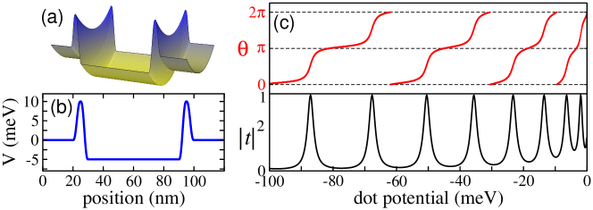
Figure 1: (color online). The adopted 2D potential profile (a) consisting of a harmonic potential with level spacing of 30 meV in the transverse direction and a double barrier along the propagation direction (b). Since no bias is applied the Fermi levels in the source and the drain coincide, and are taken to be zero. Single-particle transmission probability and phase (c) are shown, as a function of the QD potential. The energy of the incoming carriers is 1 meV.

Along the propagation direction [Fig. 1(b)], we take two smoothed barriers (with a maximum height of 10 meV and a maximum width of 10 nm) that connect a 60 nm flat negative region which mimics the QD potential which is tuned in the simulations; along the transverse direction, we consider a harmonic confinement with $\hbar\omega=$30 meV. In the setup used in Refs. Schuster et al., 1997 and Avinun-Kalish et al., 2005, no bias is applied between the QD source and drain leads since the coherent electron traversing the dot is emitted by a quantum point contact at one end of the two-path system (not included in our simulations). Accordingly, we keep the Fermi energy of the two leads at zero potential and fix the energy of the incoming electron. Material parameters for GaAs have been used. The open-boundary single-particle 2D Schrödinger equation has been solved by using the quantum transmitting boundary method Lent and Kirkner (1990) in a finite-difference scheme. Figure 1(c) shows the transmission probability and phase as a function of the QD potential. As the QD potential is varied, the incoming electron comes into resonance with higher single-particle QBLs. At each resonance peak, the phase increases by $\pi$ in agreement with the Breit-Wigner model, while it is substantially constant in the low-transmission valleys.

We show next that when the mean Coulomb field of electrons that populate the QD is taken into account, the behavior of the transmission phase shows the observed drops. In our model, the maximum of a transmission peak corresponds to the alignment of the energy of the scattered electron with the energy of a QBL of the mean-field potential. When the energy bottom of the QD is further lowered and the alignment is lost, the transmission probability decreases until the QBL becomes a genuine bound state, i.e., its energy falls below the Fermi energy, and it is occupied by an additional electron. The new mean-field potential has the QBL of the previous resonance shifted by the addition energy and, after a further lowering of the QD potential, it produces another resonance. This phenomenon, that is essentially a Coulomb blockade effect, is repeated each time a carrier is added to the QD. As the mean fields produced by $N$ or $N+1$ electrons are very similar in the large $N$ regime, the QBL that generates the resonances and the corresponding transmission phase is always the same at each peak, with an abrupt drop each time a new electron occupies a bound state of the QD.

We now apply our model to a QD with the structure potential $V_{s}$ of Figs. 1(a) and 1(b). In order to estimate the QD electrostatic potential we first solve the closed-boundary Schrödinger equation then add the field generated by an electron in the ground state $\psi_{1}$, namely

$$V_{1}(x,y)=\frac{e^{2}}{4\pi\epsilon}\int dx^{\prime}dy^{\prime}\frac{|\psi_{1}(x^{\prime},y^{\prime})|^{2}e^{-r/\lambda_{D}}}{r}$$ (1)

with $r=\sqrt{(x-x^{\prime})^{2}+(y-y^{\prime})^{2}+(d/2)^{2}}$ and where $d=1$ nm represents the thickness of the 2DEG and $\lambda_{D}=30$ nm is the Debye length not (a). The Fermi levels of the source and drain leads are fixed, i.e., we neglect the effect of the charge inside the QD on the leads. We compute the ground state of the new potential $V_{s}+V_{1}$ and we repeat the whole procedure until we reach a number $N$ of bound particles for which the potential $V_{s}+V_{1}+\dots+V_{N}$ has an unbound (positive energy) ground state. Then we compute the 2D scattering state for an incoming electron with the boundary conditions already described for the single-particle calculation. For simplicity the bound states are calculated in a finite domain by solving the closed-boundary Schrödinger equation. This leads to a shift in the energy of the bound states that has no effect on the qualitative results of the present work, i.e., the phase drops between the transmission resonances.

We show two sets of calculations in Fig. 2.

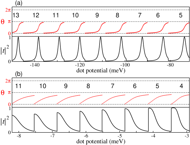
Figure 2: (color online). (a) Transmission probability and phase for an electron scattered by the potential corresponding to the sum of the structure potential described in Fig. 1 and the mean field generated by $N$ bound electrons. The numbers indicate the value of $N$ at each transmission peak: as the QD potential $V_{d}$ decreases $N$ increases. (b) Transmission probability and phase are shown for a system similar to the one of Fig. 1 whose parameters are tuned in order to match the energy levels of Ref. Avinun-Kalish et al., 2005, namely: kinetic energy of the scattered electron $\approx 20$ $\mu$eV, charging energy $\approx 1$ meV, coupling of the QD with the leads $\approx 200$ $\mu$eV, and difference between the first two single-particle QBLs $\approx 500$ $\mu$eV. The above values are obtained with a $100$ nm well and two $50$ $\mu$eV barriers $4$ nm wide in the longitudinal direction and a harmonic confinement with $\hbar\omega=1$ meV in the transverse direction.

In the top panel (a), the system parameters are chosen as in Fig. 1 in order to obtain a clear resolution of the resonances, although they do not correspond to the experiments in Refs. Schuster et al., 1997 and Avinun-Kalish et al., 2005. For the chosen parameters, the transmission occurs through the fourth excited QBL. All resonances, corresponding to different $N$, are in phase and this trend continues as the potential of the QD deepens, i.e., for larger numbers of bound electrons. Note that, although the effect of the charging of the QD is essentially classical, the transmitted electron must be obviously modeled in a quantum approach in order to obtain the transmission phase.

In Fig. 2(b), we consider a structure with parameters closer to those of the experimental conditions in Ref. Avinun-Kalish et al., 2005; in particular, the confinement potential is much weaker and the energy of the incoming electron smaller than in Fig. 2(a) (see caption), leading to less defined resonances. The transmission phase evolution is similar to the previous case, in spite of the fact that differences between the two calculations are not only quantitative, showing that the results obtained are robust against the details of the calculation and of the system. In particular, (1) due to the low energy of the incoming carrier, the transmission takes place through the ground QBL rather than an excited state; (2) the two lowest QBLs are, for $N>4$, quasi-degenerate.not (b) The latter effect is due to charge accumulation in the center of the QD, away from the barriers, inducing a double-well-like profile along the propagation direction. In this regime, the transmission peaks corresponding to the two lowest QBLs merge and, for each $N$, a single transmission resonance is found that, being originated by two quasi-degenerate states, is characterized by a phase change of $2\pi$. However, since the trapping of an additional electron in a localized state takes place just after the transmission maximum, the resulting phase evolution spans only a range of $\pi$. A further effect of the charge accumulation in the center of the QD is the decrease of the maximum value of the transmission probability on the resonances. The above trend is clear in the left part of Fig. 2(b). We note that our simulations are performed at zero temperature and with an exact energy of the incoming carriers, this leading to the steep transitions in the transmission probability of Fig. 2(b). Such steepness is not expected in experiments due to the uncertainty of the incoming carriers’ kinetic energy and the temperature dependence of bound levels’ occupancy. In the simulations based on the mean-field approach, the universal behavior, i.e. the phase drops occurring between successive resonances, persists down to $N=0$, in contrast with experiments of Ref. Avinun-Kalish et al., 2005 where phase drops may or may not occur for $N<6$. It should be noted, however, that the phase drops are a necessary consequence of the electrostatic model employed for the coupling between the bound and incoming electrons: Such a mean-field picture is expected to break down at small $N$. Indeed, we show in the following section that the inclusion of carrier correlation may give rise to an $N$-dependent phase evolution.

To conclude our mean-field analysis we discuss the similarities between the results hitherto presented and the ones obtained in Ref. Xu and Gu, 2001, also including electron-electron interaction in a mean-field approximation. In the above work, the lead-dot-lead system is modeled with a cross-bar geometry and the transmission amplitude is obtained by using the non-equilibrium Green function approach and a Hubbard Hamiltonian. The recurring phase drops are found at zeros of the transmission not (c) and persist when the electron-electron interaction is turned off. While the first effect agrees with our simulations, we find no drops in the non-interacting case. The difference can be explained by the different models adopted for the dot: a 2D double-barrier structure in our case and a 1D bar orthogonal to the lead-to-lead direction in Ref. Xu and Gu, 2001. This is confirmed by the further agreement between our Fig. 1(c) and a non-interacting simulation for a double-barrier 1D structure reported in the above work. There, the universal behavior of the transmission phase seems induced by the cross-bar configuration, with a single site between the two leads, regardless of the Coulomb interaction.

III FEW-PARTICLE APPROACH: BREIT-WIGNER AND FANO RESONANCES

In order to obtain numerically the transmission coefficient of a fully correlated system the calculation must be able to solve the few-particle problem exactly in an open domain, a difficult task for a general 2D potential. We therefore chose to simulate the dynamics for two electrons in a strictly 1D quantum wire with the same profile of Fig. 2(b); the lateral extension of the wire is, however, taken into account by an effective Coulomb potential $V_{C}(x)={e^{2}}/[4\pi\epsilon\left(x+d\right)]$, where the Coulomb singularity is smoothed by a cutoff $d=1$ nm Fogler (2005). Then, we solve exactly the few-particle open-boundary Schrödinger equation in the real space, using a generalization of the quantum transmitting boundary method mentioned above, whose general derivation is detailed elsewhere Bertoni and Goldoni (2006, 2007). In the following, we describe it for a 1D spinless system.

Let us consider a region of length $L$, with a single-particle potential $V(x)$, constant outside that region (leads): $V(x)=V(0)$ if $x<0$ and $V(x)=V(L)$ if $x>L$. Although the method is valid for the general case we consider here $V(0)=V(L)=0$ for simplicity. Let us take $(N-1)$ interacting identical particles bound by $V(x)$ in its $(N-1)$-particle ground state $\chi_{0}(x_{1},...,x_{N-1})$. The $m$-th excited eigenstates of $(N-1)$ interacting particles will be denoted by $\chi_{m}$.

Our aim is to find the correlated scattering state of $N$-particles $\psi(x_{1},\dots,x_{N})$ that has the following form when the $n$-th (with $n\leq N$) particle is localized in the left lead, i.e., when $x_{n}<0$:

$$\psi(x_{1},...,x_{n},...,x_{N})|_{x_{n}<0} = (-1)^{n}\bigg{[}\chi_{0}(x_{1},...,x_{n-1},x_{n+1},...,x_{N})e^{ik^{l}_{0}x_{n}}+$$

$$+\sum_{m=0}^{M_{l}}b^{<}_{m}\chi_{m}(x_{1},...,x_{n-1},x_{n+1},...,x_{N})e^{-ik^{l}_{m}x_{n}}+$$

$$+\sum_{m={M_{l}}+1}^{M}b^{<}_{m}\chi_{m}(x_{1},...,x_{n-1},x_{n+1},...,x_{N})e^{k^{l}_{m}x_{n}}\bigg{]},$$

where $(-1)^{n}$ accounts for the wave function antisymmetry and $k^{l}_{m}=\sqrt{|2m_{e}T_{m}|}$ represents the wave vector of the traveling particle, with mass $m_{e}$, whose kinetic energy $T_{m}=E-E_{m}$ is obtained from the total energy $E$ and the energies $E_{m}$ of the states $\chi_{m}$; in turn $E$ can be obtained from $E=T_{0}+E_{0}$ since the incoming-particle energy $T_{0}$ is the Fermi energy in the left lead.

The first term inside the square brackets on the r.h.s. of Eq. (III) accounts for the $n$-th particle incoming as a plane wave with $T_{0}$ energy from the left lead, while the other $(N-1)$ particles are in the ground state of $V$. The second term represents the linear combination of all the energy-allowed possibilities with the $n$-th particle reflected back as a plane wave in the left lead with energy $T_{m}$ and the dot in the $\chi_{m}$ state. The third term is analogous to the latter but accounts for the case $E_{m}>E$, representing the $n$-th particle as an evanescent wave in the left lead. The number of bound states whose energy is lower than the total energy, $E_{m}<E$, is $M_{l}+1$. When particle $n$ is in the right lead, the wave function has a form similar to Eq. (III), without the incoming term since we are considering only electrons traversing the dot from the left lead:

$$\psi(x_{1},...,x_{n},...,x_{N})|_{x_{n}>L} = (-1)^{n}\bigg{[}\sum_{m=0}^{M_{r}}b^{>}_{m}\chi_{m}(x_{1},...,x_{n-1},x_{n+1},...,x_{N})e^{ik^{r}_{m}x_{n}}$$ (3)

$$+\sum_{m={M_{r}}+1}^{M}b^{>}_{m}\chi_{m}(x_{1},...,x_{n-1},x_{n+1},...,x_{N})e^{-k^{r}_{m}x_{n}}\bigg{]}.$$

Since the number of interacting particles is $N$ and the problem is 1D, our computational domain consists of an $N$-dimensional hypercube that we discretize with a real-space square mesh. On the internal points, the wave function $\psi(x_{1},\dots,x_{N})$ satisfies the usual $N$-body Schrödinger equation

$$\left[-\frac{\hbar^{2}}{2m_{e}}\sum_{n=1}^{N}\frac{d^{2}}{dx_{n}^{2}}+\sum_{n=1}^{N}V_{s}(x_{n})+\sum_{n=1}^{N}\sum_{n^{\prime}=1}^{n}V_{C}(|x_{n}-x_{n^{\prime}}|)\right]\psi(x_{1},\dots,x_{N})=E\,\psi(x_{1},\dots,x_{N})\,,$$ (4)

where $V_{s}(x)$ is the 1D single-particle potential energy of the structure at position $x$ and $V_{C}(d)$ is the effective 1D Coulomb energy of two electrons at a distance $d$. $E$ is the total energy, defined previously.

The wave function $\psi$ has to match Eqs. (III) and (3) on the $N$ “left” boundaries and the $N$ “right” boundaries of the domain, respectively. Equations (III), (3) and (4) are then solved together as a coupled system of $2N+1$ equations, using a finite-difference discretization for the derivatives. In this way, the reflection amplitudes $b^{<}$ and the transmission amplitudes $b^{>}$ (i.e. the unknowns, together with $\psi$) are obtained numerically.not (d) Note that the resulting wave function is antisymmetric for any two-particle exchange since we have imposed antisymmetric boundary conditions.

Figure 3(a) shows the transmission amplitude for a two-particle correlated triplet state (bound and traveling electrons with the same spin) as a function of the QD potential.

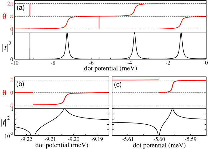
Figure 3: (color online). (a) Correlated transmission probability (bottom) and phase (top) for an electron scattered by the potential described in Fig. 2 caption when a second electron is bound in the QD. Three Breit-Wigner and two narrow Fano resonances are present. (b) and(c) Details of the transmission spectrum, with transmission probability in logarithmic scale, showing the asymmetric Fano resonances and the corresponding phase jump of $\pi$.

The energy of the incoming electron is $T_{0}=20~{}\mu$eV, as in the mean-field simulations of Sec. II. The first five transmission resonances are clearly visible, three of which have a Lorentzian shape with a width of about $200$ $\mu$eV and a Breit-Wigner-type phase evolution, similar to the ones already seen in Fig. 1. The two remaining resonances, shown in detail in Figs. 3(b) and 3(c) (note the logarithmic scale for the transmission amplitude), are very narrow (few $\mu$eV) and present a typical asymmetric Fano line shape Fano (1961). They are a signature of electron-electron correlation and, from their small width, we deduce that the effect of the Coulomb potential is very limited in our model. Nevertheless, the distinctive behavior of the transmission phase is clearly visible in the upper plots of Figs. 3(b) and 3(c). An abrupt phase jump of $\pi$ takes place near the resonance, where the transmission probability vanishes. This shows that the origin of the phase jumps detected in the few-particle experiments may reside in correlation-induced Fano resonances. A similar behavior, with the presence of both Breit-Wigner and Fano resonances, showing continuous and discontinuous phase evolutions respectively, is found in the simulation of the correlated three-electron scattering state (not shown here). In the latter case, the ratio of Fano resonances is larger and keeps increasing with the number of particles.

IV CONCLUSIONS

In summary, we showed that in the few-particle correlated regime, both Breit-Wigner and Fano resonances are found, while in the mean-field regime, a single type of resonance is present, which is repeated for each number of bound electrons, this leading to a phase jump of $\pi$ each time a new electron enters the QD. While these results are consistent with experiments, the microscopic nature of the recurring phase drops in the latter regime remains unclear. In fact, they are well reproduced by the first of our approaches in which no quantum correlation is present between the bound electrons and the scattered one. On the other hand different models hac that take into account the fully-correlated dynamics of the carrier such as our few-particle calculations cannot be applied to the many-particle regime. The above considerations suggest that in the latter regime, the coherent component of the transmitted electron wave function (i.e., the component that does not get entangled with the QD and whose phase is detected by the interferometer) behaves as if the QD, together with the bound electrons, was a static electric field, being unable to discriminate between two different values of $N$. On the other hand, when $N$ is small, the transmission phase is able to provide a partial information on the number of electrons confined in the QD through the character of the transmission resonance and the possible phase lapse. The transition regime between the many- and few-particle conditions Taniguchi and Büttiker (1999); Rontani (2006) needs further analysis since it can clarify the connections between the two opposite approaches used in the present work.

We finally note that the Fano resonances found in the 1D two-particle scattering states are a genuine effect of carrier-carrier correlation, in accordance to the original concept developed in Ref. Fano, 1961. A more general definition is often adopted, ascribing the Fano line shape of the transmittance to the interference of two alternative real-space pathways. In fact, Fano resonances have been obtained previously by means of 2D Tekman and Bagwell (1993), multi-channel Nockel and Stone (1994); Racec and Wulf (2001), and two-path Entin-Wohlman et al. (2002); Fuhrer et al. (2006) single-particle calculations. In those cases, however, the ratio between the number of Fano and Breit-Wigner resonances is not expected to vary when varying the confinement energy of the QD, while the number of correlation-induced Fano resonances becomes shortly dominant when moving from a low-$N$ to a high-$N$ condition in the framework of a full few-particle modeling.

Upon completion of this work we learned about a recent work by Karrasch et al. Karrasch et al. (2007) where the $\pi$ lapses are also ascribed to (anti)resonances of Fano type.

REFERENCES

References

- Schuster et al. (1997) R. Schuster, E. Buks, M. Heiblum, D. Mahalu, V. Umansky, and H. Shtrikman, Nature 385, 417 (1997).
- Avinun-Kalish et al. (2005) M. Avinun-Kalish, M. Heiblum, O. Zarchin, D. Mahalu, and V. Umansky, Nature 436, 529 (2005).
- Yeyati and Buttiker (1995) A. L. Yeyati and M. Buttiker, Phys. Rev. B 52, R14360 (1995).
- Ji et al. (2000) Y. Ji, M. Heiblum, D. Sprinzak, D. Mahalu, and H. Shtrikman, Science 27, 779 (2000).
- Silvestrov and Imry (2003) P. G. Silvestrov and Y. Imry, Phys. Rev. Lett. 90, 106602 (2003).
- Oreg and Gefen (1997) Y. Oreg and Y. Gefen, Phys. Rev. B 55, 13726 (1997).
- Yeyati and Buttiker (2000) A. L. Yeyati and M. Buttiker, Phys. Rev. B 62, 7307 (2000).
- Xu and Gu (2001) H. Q. Xu and B.-Y. Gu, J. Phys.: Condens. Matter 13, 3599 (2001).
- Silvestrov and Imry (2000) P. G. Silvestrov and Y. Imry, Phys. Rev. Lett. 85, 2565 (2000).
- (10) For a rewiev see G. Hackenbroich, Phys. Rep. 343, 463 (2001).
- Nockel and Stone (1994) J. U. Nockel and A. D. Stone, Phys. Rev. B 50, 17415 (1994).
- Lent and Kirkner (1990) C. S. Lent and D. J. Kirkner, J. Appl. Phys. 67, 6353 (1990).
- not (a) Although the width and energies of the resonances vary with and , we found that the qualitative behavior of the transmission amplitude is not affected by the choiche of those parameters.
- not (b) In addition, due to the very small energy of the incoming electron which is comparable to the numerical error in the determination of the energy of the QBLs, the energy where an additional electron gets trapped into the QD is fixed in the middle of the first two QBLs rather than from comparison to the Fermi energy.
- not (c) While in our case the phase drops happen as the occupancy of the dot changes by one unit and do not correspond necessarily to a zero of the transmission, in Ref. Xu and Gu, 2001, the drops always coincide with a transmission zero. This is due to the constraint of an integer occupancy in our electrostatic model.
- Fogler (2005) M. M. Fogler, Phys. Rev. Lett. 94, 56405 (2005).
- Bertoni and Goldoni (2006) A. Bertoni and G. Goldoni, J. Comp. Electron. 5, 177 (2006).
- Bertoni and Goldoni (2007) A. Bertoni and G. Goldoni (2007), (unpublished).
- not (d) The approach described replicate the “quantum transmitting boundary method” of Ref. Lent and Kirkner, 1990 and thereafter applied to the modeling of many micro- and nano-electronic systems. In fact, in the original formulation, the problem was the solution of a single-particle 2D Schrödinger equation with open boundaries, and its extension to three (and conceptually even more) dimensions was straightforward. By considering that the equation for a single particle in N dimensions and that for N particles in one dimension have the same form, it is possible to take profit of the technique developed for the former in order to solve the latter.
- Fano (1961) U. Fano, Phys. Rev. 124, 1866 (1961).
- Taniguchi and Büttiker (1999) T. Taniguchi and M. Büttiker, J. Phys.: Condens. Matter 60, 13814 (1999).
- Rontani (2006) M. Rontani, Phys. Rev. Lett. 97, 76801 (2006).
- Tekman and Bagwell (1993) E. Tekman and P. F. Bagwell, Phys. Rev. B 48, 2553 (1993).
- Racec and Wulf (2001) E. R. Racec and U. Wulf, Phys. Rev. B 64, 115318 (2001).
- Entin-Wohlman et al. (2002) O. Entin-Wohlman, A. Aharony, Y. Imry, and Y. Levinson, J. Low Temp. Phys. 126, 1251 (2002).
- Fuhrer et al. (2006) A. Fuhrer, P. Brusheim, T. Ihn, M. Sigrist, K. Ensslin, W. Wegscheider, and M. Bichler, Phys. Rev. B 73, 205326 (2006).
- Karrasch et al. (2007) C. Karrasch, T. Hecht, A. Weichselbaum, Y. Oreg, J. von Delft, , and V. Meden, Phys. Rev. Lett. 98, 186802 (2007).