Quantum phase transitions in a resonant-level model with dissipation:
Renormalization-group studies

Abstract

We study a spinless level that hybridizes with a fermionic band and is also coupled via its charge to a dissipative bosonic bath. We consider the general case of a power-law hybridization function $\Gamma(\omega)\propto|\omega|^{r}$ with $r\geq 0$, and a bosonic bath spectral function $B(\omega)\propto\omega^{s}$ with $s\geq-1$. For $r<1$ and $\mathrm{max}(0,2r-1)<s<1$, this Bose-Fermi quantum impurity model features a continuous zero-temperature transition between a delocalized phase, with tunneling between the impurity level and the band, and a localized phase, in which dissipation suppresses tunneling in the low-energy limit. The phase diagram and the critical behavior of the model are elucidated using perturbative and numerical renormalization-group techniques, between which there is excellent agreement in the appropriate regimes. For $r=0$ this model’s critical properties coincide with those of the spin-boson and Ising Bose-Fermi Kondo models, as expected from bosonization.

I Introduction

Quantum phase transitionssubirbook in mesoscopic systems form a growing area of condensed matter research. From a theoretical perspective, it is known that models of a finite system (the “impurity”) coupled to infinite baths may exhibit boundary quantum phase transitions (QPTs), at which only a subset of the degrees of freedom becomes critical.mvreview Such models help to advance our understanding of quantum criticality in strongly correlated systems: Concepts and solution techniques developed in the impurity context may be applied to lattice models, e.g., within the framework of dynamical mean-field theory (DMFT)dmft-rmp and its extensions. This approach has been followed in connection with the “local criticality” proposed to underlie the anomalous non-Fermi-liquid behavior of several heavy-fermion systems.lcqpt On the experimental side, QPTs in mesoscopic few-level systems are of great interest, both for the unprecedented opportunity to probe quantum criticality in a direct and highly controlled fashion,potok ; dias and for their numerous potential technological applications, e.g., in nanoelectronics and quantum information processing.kondo ; device ; noise

In recent years, QPTs have been identified and studied in a number of quantum impurity models.mvreview Such models can contain both fermionic bands (e.g., conduction-electron quasiparticles) and bosonic baths (e.g., phonons, spin fluctuations, or electromagnetic noise). Analytical and numerical techniques have been refined to analyze the critical behavior of these models. Analytical approaches based on bosonization or conformal field theory have been used extensively, although their applicability is limited, e.g., to certain forms of the bath spectrum. For other situations, powerful epsilon-expansion techniques have been developed. As such expansions are asymptotic in character, a comparison with numerical results is mandatory to assess their reliability.

An example with especially rich behavior is the fermionic pseudogap Kondo model,withoff which features QPTs between Kondo-screened and local-moment ground states.withoff ; cassa ; GBI ; insi ; lars ; larslong Essentially perfect agreement between the results of various epsilon expansions (around different critical dimensions) and numerical renormalization-group (NRG) calculations has been found in critical exponents as well as universal amplitudes such as the residual impurity entropy.lars ; larslong

Impurity models that include bosons are harder to tackle numerically than pure-fermionic problems due to the large Hilbert space, and fewer results are available. The development of a bosonic versionBTV ; BLTV of Wilson’s NRG approachBulla:07 has made possible a detailed nonperturbative study of the spin-boson model, where tunneling in a two-state system competes with dissipation.leggett For the case of Ohmic dissipation, the spin-boson model has long been known to display a QPT of the Kosterlitz-Thouless type. In the sub-Ohmic case, the model instead exhibits a line of continuous QPTs governed by interacting quantum critical points (QCPs).BTV ; BLTV ; VTB (The latter lie in a different universality class than the QCP of the pseudogap Kondo model.)

Of particular interest, both for mesoscopics and in the context of extended DMFT for correlated lattice-systems,edmft ; chitra are impurity models with fermionic and bosonic baths. The best-studied member of this class is the Bose-Fermi Kondo model,bfk ; sengupta ; bfknew ; kircan2 ; kirchner with a spin-$\frac{1}{2}$ local moment coupled to fermionic quasiparticles (the regular Kondo model) as well as to a bosonic bath. The latter may describe spin or charge fluctuations of the bulk system in which the impurity is embedded. The scope of NRG applications has recently been widened to provide a comprehensive treatment of an Ising-symmetric version of the Bose-Fermi Kondo model.Glossop:05 ; Glossop:07

The purpose of this paper is to investigate a somewhat simpler quantum impurity model containing both fermionic and bosonic baths, namely a resonant-level model of spinless electrons, with the impurity charge coupled to a dissipative reservoir. In standard notation, its Hamiltonian is

$$\mathcal{H} =\varepsilon_{f}f^{\dagger}f+\sum_{\bi{k}}v^{\phantom{\dagger}}_{\bi{k}}\left(f^{\dagger}c^{\phantom{\dagger}}_{\bi{k}}+\text{H.c.}\right)\,+\,\sum_{\bf{k}}\varepsilon^{\phantom{\dagger}}_{\bi{k}}c^{\dagger}_{\bi{k}}c^{\phantom{\dagger}}_{\bi{k}}$$

$$\quad+(f^{\dagger}f-\mbox{$\frac{1}{2}$})\sum_{\bi{q}}g^{\phantom{\dagger}}_{\bi{q}}(b^{\phantom{\dagger}}_{\bi{q}}+b_{-\bi{q}}^{\dagger})+\sum_{\bi{q}}\omega^{\phantom{\dagger}}_{\bi{q}}b_{\bi{q}}^{\dagger}b^{\phantom{\dagger}}_{\bi{q}}\,,$$ (1)

with $v_{\bi{k}}$ characterizing the hybridization between conduction electrons of energy $\varepsilon_{\bi{k}}$ and the impurity level at energy $\varepsilon_{f}$, and $g_{\bi{q}}$ coupling bosons of energy $\omega_{\bi{q}}$ to the impurity occupancy. Without loss of generality, $v_{\bi{k}}$ and $g_{\bi{q}}$ are taken to be real and non-negative. Equation (I) represents perhaps the simplest nontrivial Bose-Fermi quantum impurity model, making it a paradigm for this class and an ideal problem for detailed comparison between analytical and numerical results.

The model is completely specified by the impurity level energy $\varepsilon_{f}$, the hybridization function

$$\Gamma(\omega) \equiv\pi\!\sum_{\bi{k}}v_{\bi{k}}^{2}\delta(\omega\!-\!\varepsilon_{\bi{k}})=\Gamma_{0}\left|\frac{\omega}{D}\right|^{r} \!\!\!\!\text{for }|\omega|<D,$$ (2)

and the bosonic bath spectral function

$$B(\omega) \equiv\pi\!\sum_{\bi{q}}g_{\bi{q}}^{2}\delta(\omega\!-\!\omega_{\bi{q}})=B_{0}\left(\frac{\omega}{\omega_{c}}\right)^{\!\!s} \!\!\!\!\text{for }0<\omega<\omega_{c},$$ (3)

with $D$ and $\omega_{c}$ acting as fermionic and bosonic cutoffs, respectively. Thus, in addition to a power-law spectrum for the bosonic bath density of states (DOS) characterized by an exponent $s$, we consider a nonconstant particle-hole (p-h) symmetric hybridization function characterized by an exponent $r$. Increasing $r$ (and hence depleting the hybridization function around the Fermi level $\omega=0$) and increasing $B_{0}$ both act to suppress tunneling between the local level and the conduction band. For most of the numerical work presented in Sec. III, we fix $r$, $s$, and the hybridization strength $\Gamma_{0}$, then tune the dissipation strength $B_{0}$ to the vicinity of a QPT.

Although the bath densities of states and $v_{\bi{k}}$, $g_{\bi{q}}$ do not require separate specification, it will facilitate comparison between numerical and perturbative results to assume that $v_{\bi{k}}=v_{0}$, $g_{\bi{q}}=g_{0}$ for all $\bi{k}$, $\bi{q}$. In this case, $\Gamma(\omega)=\pi v_{0}^{2}\rho_{c}(\omega)$ and $B(\omega)=\pi g_{0}^{2}\rho_{b}(\omega)$, with the fermionic and bosonic DOS given, respectively, by

$$\rho_{c}(\omega) =N_{0}\left|\omega/D\right|^{r} \text{for }|\omega|<D\,,$$ (4)

$$\rho_{b}(\omega) =(K_{0}^{2}/\pi)\left(\omega/\omega_{c}\right)^{s} \text{for }0<\omega<\omega_{c}\,,$$ (5)

where $N_{0}$ and $K_{0}$ are normalization factors. Thus, $\Gamma_{0}=\pi N_{0}v_{0}^{2}$ and $B_{0}=(K_{0}g_{0})^{2}$. The metallic case is recovered for $r=0$, and Ohmic dissipation corresponds to taking $s=1$.

It is convenient to identify a pseudospin—making clear the close relationship between model (I) and the spin-boson model and its variants—by writing

$$f^{\dagger}\equiv S^{+},\quad f\equiv S^{-},\quad f^{\dagger}f-\frac{1}{2}\equiv S_{z}\,.$$ (6)

In the model described by Eq. (I), the friction caused by the bosonic bath competes with the resonant tunneling of electrons. In contrast to the simpler spin-boson model,leggett the tunneling properties are determined by the hybridization function $\Gamma(\omega)$.

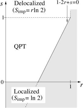
Figure 1: Schematic phase diagram of the dissipative resonant-level model (I), in the parameter space spanned by exponents $r$ and $s$ characterizing the low-energy behavior of fermionic and bosonic baths, respectively. (A finite coupling to both baths is assumed.) For $\text{max}(0,2r-1)<s\leq 1$, the model shows a boundary quantum phase transition (as the couplings $v_{0}$ and $g_{0}$ are varied) between a delocalized phase and a localized phase. (The physics along the line $r=0$ is identical to that of the spin-boson model.) In contrast, for $s>1$ and $r<1$ the system is generically delocalized, whereas it is localized in the rest of the parameter regime (shaded). The impurity entropy $S_{\text{imp}}$ is discussed in the text. Two perturbative RG expansions are employed: around the free-impurity fixed point, where the expansion is controlled about $r=s=1$ (Sec. II.2) and around the resonant-level fixed point, where the expansion is controlled in $1-2r+s$ (Sec. II.3).

For $\varepsilon_{f}=0$ the model features a Z₂ symmetry of particle-hole type [assuming $\rho_{c}(\omega)=\rho_{c}(-\omega)$ as noted above], namely $c{k}\rightarrow c{k}^{\dagger}$, $f\rightarrow-f^{\dagger}$, and $S_{z}\rightarrow-S_{z}$. Then, we expect that the competition between resonant tunneling and dissipation yields a QPT between a “delocalized” phase ($\langle S_{z}\rangle=0$), in which the principal effect of dissipation is to renormalize the tunneling amplitude, and a “localized” phase ($\langle S_{z}\rangle\neq 0$) with a doubly degenerate ground state, where the tunneling amplitude renormalizes to zero in the low-energy limit. We note that for the case of a metallic fermionic bath [$r=0$ in Eq. (4)], bosonization techniques can be used to map the model (I) to the spin-boson model.hur1 (The same applies to the Ising-symmetric Bose-Fermi Kondo model with $r=0$, and this equivalence has been verified using NRG.Glossop:05 ; Glossop:07 )

In this paper, we employ renormalization-group (RG) techniques to map out the phase diagram of the Hamiltonian (I) and to establish over what range of bath exponents $r$ and $s$ the model can be tuned to a delocalized-to-localized QPT, akin to that of the spin-boson model. We do so using both perturbative RG methods, based on epsilon-expansion techniques developed in the context of the pseudogap Kondo and Anderson models,larslong and the Bose-Fermi extensionGlossop:05 ; Glossop:07 of the NRG approach, which allows us to access the entire parameter range of the model.

Our main result is summarized in Fig. 1, which illustrates the qualitative behavior of the model in the plane spanned by the bath exponents $r$ and $s$. A delocalized-to-localized transition—which for $r=0$ is identically that of the spin-boson model—is present at $r>0$ as well. A more detailed discussion is given in Sec. II.3.3.

The remainder of the paper is organized as follows. The perturbative RG analysis is outlined in Sec. II, where results for various critical exponents are obtained by expansion around two distinct fixed points. In Sec. III, we provide nonperturbative NRG results for the model, including discussion of the phase diagram, the response to a local field, and the single-particle spectral function. We find excellent quantitative agreement between analytical and numerical results in the appropriate limits. Although the critical properties of the model (I) for $r=0$ are established via the mapping to the spin-boson model, we confirm the equivalence by direct calculation.

II Perturbative renormalization group

II.1 Zero-temperature phases

We begin by discussing the trivial fixed points of the model (I) in the presence of p-h symmetry, $\varepsilon_{f}=0$. As a characterization, we will refer to the residual impurity entropy $S_{\rm imp}$, which is defined as the impurity contribution to the total entropy in the limit temperature $T\to 0$.mvreview

For $v_{0}=g_{0}=0$, the impurity is decoupled from both baths. We denote this free-impurity fixed point by FImp. The ground state is doubly degenerate: $S_{\text{imp}}=\ln 2$.

For $v_{0}\neq 0$ and $g_{0}=0$ one has a resonant-level model with a power-law conduction-band DOS given by Eq. (4). The hybridization is relevant in the RG sense (w.r.t. FImp) for $r<1$, and hence the impurity charge strongly fluctuates.GBI ; larslong We refer to this as the delocalized fixed point (Deloc), which, as discussed in Ref. larslong, , is located at intermediate RG coupling, $(g,v)=(0,v^{\ast})$. Somewhat surprisingly, the impurity entropy is $S_{\text{imp}}=r\ln 2$, and vanishes only in the metallic case $r=0$. For $r>1$, by contrast, the hybridization is RG-irrelevant, and the delocalized fixed point merges with FImp.spinfoot

The dissipative coupling $g_{0}$ turns out to be RG-relevant at the FImp fixed point for $s<1$ (see, e.g., Refs. leggett, and BTV, ). It tends to suppress tunneling in the low-energy limit. By analogy with the spin-boson model, this can be expected to result in a doubly degenerate ground state, $S_{\text{imp}}=\ln 2$, i.e., a phase with broken $Z_{2}$ symmetry. This localized fixed point (Loc) corresponds to coupling values $(g,v)=(\infty,0)$. (Note that for $s>1$ the effect of the bosonic bath is weak, not causing localization.)

The preceding discussion suggests that, for $r<1$ and $s<1$, a QPT separates a delocalized (small-dissipation) phase from a localized (large-dissipation) phase. Clearly, this applies only to the case of p-h symmetry, $\varepsilon_{f}=0$. Otherwise the $Z_{2}$ symmetry of the Hamiltonian is broken from the outset, and the phase transition upon variation of the dissipation strength will be smeared into a crossover; this is analogous to the behavior of the spin-boson model in the presence of a finite bias. Furthermore, in situations where the system is localized at $\varepsilon_{f}=0$, there will be a first-order transition upon tuning $\varepsilon_{f}$ from positive to negative values (as in an ordered magnet subject to a field).

We now proceed with an RG treatment of the model (I), carried out without recourse to bosonization. We can access quantum-critical properties via two distinct expansions: (i) an expansion around the free-impurity fixed point (Sec. II.2), which is formally valid provided that the couplings to both baths are small, and (ii) an expansion around the resonant-level fixed point (Sec. II.3), performed after exactly integrating out the $c$ fermions. The second approach proves to have the wider range of applicability.

II.2 RG expansion around the free-impurity limit

In this subsection, we apply an RG epsilon expansion for weak couplings near the free-impurity fixed point where $v_{0}=g_{0}=0$.

II.2.1 RG equations

We model the bosonic bath by a relativistic scalar field, $\phi=b+b^{\dagger}$, in $d=2+s$ dimensions, with the action

$$\mathcal{S}_{\phi}=\int_{0}^{\beta}\!\!d\tau\int^{\Lambda_{q}}\!\!\frac{d^{d}\bi{q}}{(2\pi)^{d}}\,\phi_{-\bi{q}}(\tau)\left(-\partial_{\tau}^{2}+\bi{q}^{2}\right)\phi{q}(\tau),$$ (7)

$\Lambda_{q}$ being a momentum-space cutoff (related to the energy cutoff $\omega_{c}$ via $\omega_{c}=c\Lambda_{q}$ with $c=1$ being a velocity). This produces a DOS of the form

$$\rho_{\phi}(\omega)=\text{sgn}(\omega)\frac{S_{2+s}}{2}|\omega|^{s}=\text{sgn}(\omega)\frac{K_{0}^{2}}{\pi}\left|\frac{\omega}{\omega_{c}}\right|^{s},$$ (8)

for $|\omega|<\omega_{c}$, with $S_{d}=2/[(4\pi)^{d/2}\Gamma(d/2)]$. [Note that $\rho_{\phi}$ is just a symmetrized version of $\rho_{b}$ defined in Eq. (5).] Similarly, we represent the fermionic bath by Dirac fermions in $(1+r)$ dimensions:

$$\mathcal{S}_{c}=\int_{0}^{\beta}\!\!d\tau\int_{-\Lambda_{k}}^{\Lambda_{k}}\frac{dk|k|^{r}}{(2\pi)^{1+r}}\,{\bar{c}}_{k}(\partial_{\tau}+k)c_{k}\,,$$ (9)

with $\Lambda_{k}=D/v_{F}$ and $v_{F}=1$ being the (Fermi) velocity, which reproduces the DOS defined in Eq. (4). A path-integral representation of Eq. (I) reads

$$\mathcal{S} =\mathcal{S}_{c}+\mathcal{S}_{\phi}+\int_{0}^{\beta}\!\!d\tau\bar{f}\>\partial_{\tau}f+g_{0}\int_{0}^{\beta}\!\!d\tau\,({\bar{f}}f-\mbox{$\frac{1}{2}$})\,\phi(\tau,0)$$

$$\quad+v_{0}\int_{0}^{\beta}\!\!d\tau\left[\bar{f}c(\tau,0)+\text{c.c.}\right].$$ (10)

Power counting yields the bare scaling dimensions of fields and couplings with respect to $v_{0}=g_{0}=0$: $[f]=0$, $[\phi_{\bi{q}}]=-(1+s)/2$, $[c{k}]=-(1+r)/2$, $[v_{0}]=(1-r)/2$, and $[g_{0}]=(1-s)/2$. Thus, we can carry out an RG expansion around $r=1$ and $s=1$, where both $v_{0}$ and $g_{0}$ become marginal, defining

$$\epsilon=\frac{1}{2}(1-s),\quad\epsilon^{\prime}=\frac{1}{2}(1-r).$$ (11)

In order to proceed with the RG analysis, we define a renormalized field $f_{R}$ and couplings $v$ and $g$ according to

$$\begin{split}f&=\sqrt{Z_{f}}f_{R}\,,\\ v_{0}&=\mu^{\epsilon^{\prime}}\sqrt{\frac{D^{r}}{N_{0}Z_{f}}}Z_{v}v\,,\\ g_{0}&=\mu^{\epsilon}\frac{\sqrt{\omega_{c}^{s}\pi}Z_{g}}{K_{0}Z_{f}}g\,,\end{split}$$ (12)

where $\mu$ is an arbitrary renormalization energy scale and $Z_{f}$, $Z_{v}$, and $Z_{g}$ are renormalization factors. As is usual for impurity problems, there is no renormalization of the bosonic and fermionic bulk propagators, since the impurity only provides a one-over-volume correction to the bulk properties. The relevant diagrams for obtaining the one-loop RG beta functions are shown in Fig. 2.

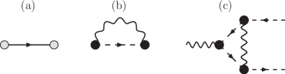
Figure 2: Diagrams appearing in the perturbative expansion for the dissipative resonant-level model. Dashed, solid, and wiggly lines denote respectively $f$, $c$, and $\phi$ propagators. The gray (black) circles are the interaction vertices $v$ ($g$). (a) and (b): $f$ fermion self-energy diagrams to one-loop order. (c) One-loop vertex renormalization of $g$.

Following standard procedures,bgz the one-loop RG beta functions of the dissipative resonant-level model are given by

$$\begin{split}\beta(v)&=-\epsilon^{\prime}v+v^{3}+\mbox{$\frac{1}{2}$}g^{2}v\,,\\ \beta(g)&=-\epsilon g+2v^{2}g\,,\end{split}$$ (13)

where the calculation parallels that of Ref. larslong, . The corresponding $Z$ factors, to one-loop accuracy, are $Z_{f}=1-v^{2}/\epsilon^{\prime}-g^{2}/2\epsilon$, $Z_{v}=1$, and $Z_{g}=1-g^{2}/2\epsilon$.

The RG flows arising from Eqs. (13) are plotted in Fig. 3. In this subsection, we consider the case $0<s<1$; the regime $s<0$ is discussed in Sec. II.3.2. Fixed points at $(g^{\ast\,2},v^{\ast\,2})=(0,\epsilon^{\prime})$ and $(g^{\ast\,2},v^{\ast\,2})=(\infty,0)$ describe the delocalized (Deloc) and localized (Loc) phases, respectively. For $r<r_{+}$, where

$$r_{+}=(1+s)/2,$$ (14)

both these fixed points are stable: For small $g_{0}$ and large $v_{0}$, the ground state is delocalized, characterized by strong local charge fluctuations due to resonant tunneling between the impurity and the conduction electron bath ($\langle S_{z}\rangle=0$). In the opposite limit of small $v_{0}$ and large $g_{0}$, we find a localized ground state where charge tunneling renormalizes to zero in the low-energy limit ($\langle S_{z}\rangle\neq 0$). An unstable critical fixed point [Cr], located at $(g^{\ast\,2},v^{\ast\,2})=(2\epsilon^{\prime}-\epsilon,\epsilon/2)$, controls the QPT between these two phases. This critical fixed point lies on the separatrix specifying the phase boundary in the $g_{0}$-$v_{0}$ plane between the delocalized and localized phases.

As $r$ approaches $r_{+}$ from below, the critical fixed point merges with the delocalized fixed point (which itself merges with FImp as $r\to 1$ from below). Hence, no transition occurs for $r\geq r_{+}$: Deloc and FImp are unstable w.r.t. infinitesimal bosonic coupling, such that the ground state is always localized for $g_{0}\neq 0$.

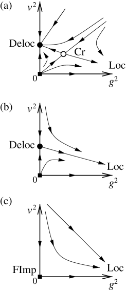
Figure 3: Schematic RG flow diagrams for the dissipative resonant-level model with p-h symmetry. Although these diagrams are obtained by expansion about the free-impurity fixed point and hence are formally valid as $r,s\to 1$, they are confirmed by expansion about the delocalized fixed point (Sec. II.3) and NRG calculations (Sec. III) to capture the correct physics for all $r\geq 0$ and $0<s<1$. The horizontal axis denotes the renormalized bosonic coupling $g$; the vertical axis denotes the renormalized hybridization $v$. (a) $r<r_{+}=(1+s)/2$: Stable fixed points at Deloc and Loc describe the delocalized and localized phases, respectively. The continuous impurity QPT is controlled by the critical fixed point Cr. (b) $r_{+}<r<1$: The delocalized (Deloc) fixed point is unstable against finite $g$. As $r\to 1^{-}$, the Deloc fixed point merges with the free-impurity fixed point (FImp). (c) $r\geq 1$: $v$ is irrelevant. In both (b) and (c), the flow is toward Loc for any finite $g$.

II.2.2 Correlation-length exponent

In the following, we discuss the properties of the boundary QPT, controlled by the critical fixed point Cr. We start with the correlation-length exponent $\nu$, describing the flow away from criticality: The characteristic energy scale $T^{*}$ above which quantum-critical behavior is observed vanishes assubirbook

$$T^{*}\propto|t|^{\nu}\,,$$ (15)

where $t$ is a dimensionless measure of the distance to criticality, defined such that $t>0$ ($t<0$) corresponds to the localized (delocalized) phase. Upon linearization of the RG beta functions around the Cr fixed point, we obtain

$$\frac{1}{\nu}=\sqrt{\frac{\epsilon^{2}}{4}+4\epsilon\left(\epsilon^{\prime}-\frac{\epsilon}{2}\right)}-\frac{\epsilon}{2}+\mathcal{O}\left(\epsilon^{2},\epsilon^{\prime\,2}\right)\,.$$ (16)

Clearly, $\nu$ diverges as $s\to 1$ and $r\to 1$ together. By expanding the square-root in Eq. (16), the inverse correlation length exponent can be approximated as $\nu^{-1}=1-2r+s$. The same result, valid for small $1-2r+s$, is also obtained in Sec. II.3 following an RG expansion valid near the strong-coupling fixed point. The divergence of $\nu$ as $1-2r+s\to 0$ is demonstrated numerically in Sec. III.2.1 and the form compared to Eq. (16).

II.2.3 Response to a local field

The local impurity susceptibility $\chi_{\text{loc}}(T)$ is the impurity response to a field applied only to the impurity.mvreview Here, for the spinless resonant-level model under consideration, the level energy $\epsilon_{f}$ plays the role of a local electric field. Defining the impurity “magnetization” $m_{\text{imp}}=\langle S_{z}\rangle$, with the pseudospin $S_{z}$ as specified in Eq. (6), it follows that

$$\chi_{\text{loc}}=-\frac{\partial m_{\text{imp}}}{\partial\varepsilon_{f}}$$ (17)

is nothing other than the impurity capacitance.

Near criticality, $\chi_{\text{loc}}(T)$ is expected to follow a power-law form

$$\chi_{\text{loc}}(T)\propto\frac{1}{T^{1-\eta_{\chi}}}\quad\text{for }T^{*}\ll T\ll T_{0},$$ (18)

up to a nonuniversal cutoff scale $T_{0}$. This relation defines the anomalous exponent $\eta_{\chi}$, which governs the anomalous decay of the impurity “spin-spin” correlation function and is calculated via

$$\eta_{\chi}=\mu\frac{\partial\ln Z_{\chi}}{\partial\mu}\bigg{|}_{v^{\ast},g^{\ast}}\,.$$ (19)

The renormalization factor $Z_{\chi}$ obeys the exact relationmvreview ; bfknew

$$Z_{\chi}^{-1}=(Z_{g}/Z_{f})^{2}\,,$$ (20)

which is graphically represented in Fig. 4(a). This allows us to derive the exact result

$$\eta_{\chi}=2\epsilon=1-s$$ (21)

at the Cr fixed point, a relation that is borne out by the numerical results presented in Sec. III.

II.2.4 Conduction electron $T$-matrix

The conduction electron $T$-matrix, describing the scattering of the $c$ electrons off the impurity, is another important observable, being central to the calculation of transport properties. For a resonant-level model, the $T$-matrix is given by $T(\omega)=v_{0}^{2}G_{f}(\omega)$ where $G_{f}$ is the full impurity ($f$-electron) Green’s function, graphically represented in Fig. 4(b). As with the local susceptibility, we expect a power-law behavior of the $T$-matrix spectral density near criticality:

$$T(\omega)\propto\frac{1}{|\omega|^{1-\eta_{T}}}\quad\text{for }T^{*}\ll|\omega|\ll T_{0}\,.$$ (22)

It has been shownlarslong that all critical fixed points for $0<r<1$ in the pseudogap Anderson and Kondo models display $T(\omega)\propto|\omega|^{-r}$ as $\omega\to 0$, which behavior has been observed in a number of separate studies.Bulla:97 ; Logan:00 ; Bulla:00

Using the exact relation $Z_{T}=Z_{f}/Z_{v}^{2}$, we can derive an exact result for the critical point of the dissipative resonant level model:

$$\eta_{T}=1-r\,.$$ (23)

Thus, even though the multiplicative prefactor of the behavior (22) is expected to exhibit both $r$ and $s$ dependence, the power law followed at criticality is identical to that of the pseudogap Kondo and Anderson models.

II.2.5 Hyperscaling and other critical exponents

The QCP is expected to satisfy hyperscaling relations characteristic of an interacting fixed point, including $\omega/T$ scaling in dynamical quantities.mvreview It follows that the correlation-length exponent $\nu$ and the anomalous exponent $\eta_{\chi}$ are sufficient to determine all critical exponents associated with the application of a local field.insi ; mvreview For example, one can define exponents $\gamma$ and $\gamma^{\prime}$ through the $T\to 0$ limit of the local susceptibility near criticality:

$$\begin{gathered}\chi_{\text{loc}}(t<0;T=0)\propto(-t)^{-\gamma},\;\;\;\gamma=\nu(1-\eta_{\chi})\,,\\ T\chi_{\text{loc}}(t>0;T=0)\propto t^{\gamma^{\prime}},\;\;\;\gamma^{\prime}=\nu\eta_{\chi}\,.\end{gathered}$$ (24)

One can also determine critical exponents $\beta$ and $\delta$ associated with the local magnetization $m_{\text{imp}}$:

$$\begin{gathered}m_{\text{imp}}(t>0;T=0,\varepsilon_{f}\to 0)\propto t^{\beta},\;\;\;\beta=\nu\eta_{\chi}/2,\\ m_{\text{imp}}(\varepsilon_{f};t=0,T=0)\propto|\varepsilon_{f}|^{1/\delta},\;\;\;\delta=2/\eta_{\chi}-1.\end{gathered}$$ (25)

Thus, near criticality

$$\beta=\frac{\epsilon}{\sqrt{\epsilon^{2}/4+4\epsilon(\epsilon^{\prime}-\epsilon/2)}-\epsilon/2}+\mathcal{O}\left(\epsilon^{2},\epsilon^{\prime\,2}\right)$$ (26)

and

$$\delta=\frac{1}{\epsilon}-1+\mathcal{O}\left(\epsilon^{2},\epsilon^{\prime\,2}\right),$$ (27)

where, in contrast to Eqs. (21) and (23), the higher-order corrections do not cancel. Section III reports NRG results for several of these critical exponents that demonstrably obey the hyperscaling relations.

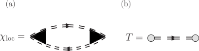
Figure 4: (a) Exact relation for the local susceptibility. The black triangle denotes the full vertex function and the dashed double line denotes the full impurity level propagator. (b) The large dot denotes the full hybridization vertex.

II.3 RG expansion around the delocalized fixed point

In addition to the RG expansion for $r\to 1$ and $s\to 1$, as described in Sec. II.2, a second epsilon expansion can be performed around the Deloc fixed point.

II.3.1 RG equations

To begin, we integrate out the conduction electrons, which is an exact operation for the present model. The resulting action islarslong

$$\mathcal{S} =\sum_{\omega_{n}}{\bar{f}}(\omega_{n})\,\bigl{[}iA_{0}\text{sgn}(\omega_{n})|\omega_{n}/D|^{r}+iA_{1}\omega_{n}\bigr{]}\,f(\omega_{n})$$

$$\quad+\mathcal{S}_{\phi}+g_{0}\int_{0}^{\beta}\!\!d\tau\left({\bar{f}}f-\mbox{$\frac{1}{2}$}\right)\phi(\tau,0)\,,$$ (28)

where the local $f$ fermions are now “dressed” by the conduction lines,

$$A_{0}=\pi N_{0}v_{0}^{2}\sec\left(\frac{\pi r}{2}\right)=\Gamma_{0}\sec\left(\frac{\pi r}{2}\right)$$ (29)

is a nonuniversal energy scale, and $A_{1}=1+\mathcal{O}(v_{0}^{2})$. For $r<1$, the $|\omega_{n}|^{r}$ term dominates the $f$ propagator at low energies. Then, dimensional analysis of the bosonic coupling (here w.r.t. the Deloc fixed point) yields

$$[g_{0}]=\frac{2r-1-s}{2}\,,$$ (30)

which implies that an RG expansion can be controlled in the smallness of

$$2\tilde{\epsilon}=1-2r+s.$$ (31)

We introduce a dimensionless coupling according

$$g_{0}=\mu^{-\tilde{\epsilon}}A_{0}\frac{\sqrt{\omega_{c}^{s}\pi}Z_{g}}{K_{0}Z_{f}}g\,,$$ (32)

and, following the procedure described in Sec. II.2, we find that the only contribution to $Z_{g}$ is that shown in Fig. 2(c), which reads (note that $Z_{f}=1$ to this order)

$$Z_{g}=1+\csc\!\left(\frac{\pi s}{2}\right)\frac{g^{2}}{\tilde{\epsilon}}\,.$$ (33)

The RG beta function for $g$ is

$$\beta(g)=\tilde{\epsilon}g-2\csc\!\left(\frac{\pi s}{2}\right)g^{3}.$$ (34)

It is clear from Eq. (34) that for $s>0$ and $\tilde{\epsilon}>0$, there exists a critical fixed point at

$$g^{\ast\,2}=\frac{\tilde{\epsilon}}{2}\sin\left(\frac{\pi s}{2}\right)\,,$$ (35)

which controls the delocalized-to-localized transition. The RG flow diagram is sketched in Fig. 5.

Note that the critical coupling $g^{\ast}$ approaches zero as $\tilde{\epsilon}\to 0^{+}$ and/or as $s\to 0^{+}$, suggesting that beyond these limiting cases the delocalized fixed point is unstable towards the localized fixed point. The same instability has already been deduced for $\tilde{\epsilon}<0$ [i.e., for $r>r_{+}=(1+s)/2$], based on expansion about the free-impurity fixed point (see Sec. II.2). The behavior for $s\leq 0$ is analyzed in the next section.

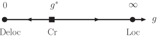
Figure 5: RG flow diagram of the dissipative resonant-level model near the delocalized (Deloc) fixed point for $s$, $\tilde{\epsilon}>0$. The two stable phases are governed by the delocalized ($g=0$) and localized ($g=\infty$) fixed points, separated by the critical fixed point [$g=g^{\ast}$ specified in Eq. (35)].

II.3.2 The regime $s\leq 0$

For $s\leq 0$, the perturbation theory described in Sec. II.3 is singular due to the divergent DOS in the bosonic propagator. In this range of $s$, the delocalized fixed point is always unstable against any infinitesimal bosonic coupling $g_{0}$, which favors the localized fixed point.

We can gain a better understanding of this instability by considering the local bosonic propagator $G_{\phi_{0}}(i\omega_{n})=\sum{q}G_{\phi}(\bi{q},i\omega_{n})$ in the presence of the impurity. Including impurity effects via the boson self-energy, the local boson propagator is given by

$$G^{-1}_{\phi_{0}}(i\omega_{n})=\left\{\begin{array}[]{ll}\omega_{n}^{s}+s\Lambda^{s}-g_{0}^{2}&\text{for }s>0,\\[4.30554pt] \omega_{n}^{-s}-g_{0}^{2}&\text{for }s\leq 0,\end{array}\right.$$ (36)

where $\Lambda$ is a momentum cutoff energy scale. Let us discuss $s>0$ first. For $s\Lambda^{s}>g_{0}^{2}>0$, the local boson propagator is massive, meaning that the ground state for the bulk is just the empty state. For $g_{0}^{2}>s\Lambda^{s}>0$, by contrast, the local boson propagator has “negative mass”, as a consequence of which the local boson condenses at zero temperature with an expectation value $\langle\phi_{0}\rangle\neq 0$. This drives the system to the localized phase where the pseudospin operator $S_{z}$ also assumes a nonzero expectation value. This reasoning supports the existence of a QPT for $s>0$, with criticality reached at $g^{\ast\,2}=s\Lambda^{s}$. For $s\leq 0$, the local boson propagator $G_{\phi_{0}}$ always has a negative mass, i.e., the impurity is localized. (Technically, the impurity induces a bound state in $G_{\phi_{0}}$.) The observation that the ground state is always localized for $s\leq 0$ is consistent with previous studies of the spin-boson modelBTV ; VTB and the Bose-Fermi Kondo model,Glossop:05 ; Glossop:07 which belong to the same universality class as the dissipative resonant-level model in the metallic limit $r=0$.

II.3.3 Phase diagram

The RG flow allows us to deduce that the qualitative phase diagram of the dissipative resonant-level model in the parameter space specified by $r$ and $s$ is as shown in Fig. 1. The solid line denotes the locus of points satisfying $1-2r+s=0$. In the unshaded region to the left of the line [i.e., for $\text{max}(0,2r-1)<s<1$, or equivalently $\mbox{$\frac{1}{2}$}<r_{+}<r<1$ with $r_{+}$ defined in Eq. (14)], the RG expansion predicts a continuous QPT as $v_{0}$ and $g_{0}$ are varied. For $s<\text{max}(0,2r-1)$ (shaded area), the ground state of the model is always localized for any finite bosonic coupling $g_{0}$. This is consistent with the RG flow diagrams presented in Fig. 3, where the RG expansion is carried out for $r,s\to 1$. The phase diagram is confirmed by NRG results in Sec. III.

II.3.4 Critical exponents

By linearizing the RG equation around the fixed point, the correlation-length exponent at the critical point $g^{\ast}$ is found to satisfy

$$\frac{1}{\nu}=2\tilde{\epsilon}+\mathcal{O}\left(\tilde{\epsilon}^{2}\right).$$ (37)

For the anomalous exponent $\eta_{\chi}$ associated with the local susceptibility [Eq. (18)], we again have the exact property Eq. (20) [see also Fig. 4(a)], from which it follows that

$$\eta_{\chi}=1-s\,.$$ (38)

The exponents $\beta$ and $\delta$ can be obtained from the hyperscaling relations (25):

$$\beta=\frac{1-s}{4\tilde{\epsilon}}+\mathcal{O}\left(\tilde{\epsilon}^{2}\right),$$ (39)

and

$$\delta=\frac{1+s}{1-s}+\mathcal{O}\left(\tilde{\epsilon}^{2}\right).$$ (40)

The exponent $\eta_{T}$, associated with conduction-electron $T$-matrix, is also found to obey $\eta_{T}=1-r$ [see Eq. (23)]. Of course, all critical exponents for the two RG expansions (one for $r,s\to 1$ and one for $1-2r+s\to 0$) are expected to be compatible since the expansions describe the same QPT. In the limit $r,s\to 1$, the square root of Eq. (16) may be expanded to yield Eq. (37). The equivalences of Eqs. (26) and (39) for $\beta$ and of Eqs. (27) and (40) for $\delta$ are also readily verified.

III Numerical renormalization group

The NRG methodBulla:07 has recently been extended to provide nonperturbative results for the Bose-Fermi Kondo model.Glossop:05 ; Glossop:07 In the following, we implement the same approach for the spinless resonant-level model (I), which also involves both fermionic and bosonic baths.

Figure 6: (Color online) (a) The lowest NRG eigenstates $E_{N}$ vs even iteration number $N$ for $(r,s)=(0.85,0.9)$, hybridization strength $\Gamma_{0}=0.1$, and a range of dissipation strengths $B_{0}-B_{0,c}=0,\pm 10^{-3},\pm 10^{-2}$. The flows are typical of those for $\text{max}(0,2r-1)<s<1$ with $0\leq r<1$. The levels at the critical coupling $B_{0}=B_{0,c}\approx 0.3731$ are shown as bold dotted lines while those nearby in the delocalized ($B_{0}<B_{0,c}$) [localized ($B_{0}>B_{0,c}$)] phase are shown as solid [dashed] lines. As $B_{0}$ approaches $B_{0,c}$ in either phase, the levels follow those of the unstable critical fixed point down to progressively lower temperatures, before crossing over to the levels characteristic of the delocalized or localized stable fixed point. (b) NRG level flows for $(r,s)=(0.975,0.9)$. In this case, and more generally for $s<\text{max}(0,2r-1)$ with $0\leq r<1$, the flow is towards the localized fixed point for any $B_{0}>0$, but follows the delocalized fixed point down to progressively lower temperatures as $B_{0}$ is reduced towards zero. The solid lines show the flow for $B_{0}=0$.

There are three essential features of the NRG: (i) The energy axis is logarithmically discretized, introducing a discretization parameter $\Lambda$. (ii) The Hamiltonian is then mapped to a chain form, with the impurity degrees of freedom coupled to the first site only of one or more tight-binding chains. (iii) Owing to the discretization, the tight-binding coefficients decay exponentially with increasing chain length. This allows the problem to be solved in an iterative fashion, diagonalizing progressively longer finite-length chains and thereby including exponentially smaller energy scales, $T_{N}\approx D\Lambda^{-N/2}$, at each iterative step $N=0$, $1$, $2$, $\ldots$. The RG transformation relating the effective Hamiltonians at consecutive iterations eventually reaches a scale-invariant fixed point that determines the low-temperature properties of the system.

In all applications of the NRG, the maximum number $N_{s}$ of many-body eigenstates retained from iteration $N$ to form basis states for iteration $N+1$ must be truncated for sufficiently large $N$ due to the limitations of finite computational power. The presence of one or more bosonic chains introduces additional considerations. First, the bosonic Hilbert space must be truncated even at iteration $N=0$, allowing a maximum of $N_{b}$ bosons per site of a bosonic chain. Second, for problems involving both fermionic and bosonic chains, the fact that the bosonic tight-binding coefficients decay as the square of those for fermionic chains must be reflected in the specific iterative scheme employed. That is, only (bosonic and fermionic) excitations of the same energy scale should be considered at the same iterative step. Thus, while the fermionic chain is extended at each iteration, the bosonic chain is extended only at every second iteration. These issues, together with further details of the implementation of the Bose-Fermi NRG, are discussed in detail in Ref. Glossop:07, .

The NRG method has provided a comprehensive numerical account of the quantum-critical properties of a number of impurity problems, e.g., the fermionic pseudogap Kondo and Anderson models, the spin-boson model, and the Bose-Fermi Kondo model. In all cases it is found that the critical properties (such as exponents) are insensitive to the discretization parameter $\Lambda$ and converge rapidly with the number of retained states $N_{s}$. For models involving bosonic baths, critical exponents also rapidly converge with increasing bosonic truncation parameter $N_{b}$. In the following we take $\Lambda=3$, with all data suitably converged for the choice $N_{s}=500$ and $N_{b}=8$. For convenience we set $D=\omega_{0}=1$.

III.1 Phase diagram

Figure 6 shows the flow of the lowest NRG eigenstates $E_{N}$ of the effective Hamiltonian $H_{N}$ at even iteration numbers $N$ for two representative cases for $s>0$: (a) $1-2r+s>0$ and (b) $1-2r+s<0$. Figure 6(a) shows data obtained for $(r,s)=(0.85,0.9)$ and $\Gamma_{0}=0.1$. Here, and for any $1-2r+s>0$, the flow is schematized by Fig. 3(a), which follows from the perturbative analysis. For $B_{0}<B_{0,c}$, the NRG flow is towards the delocalized fixed point, where the spectrum coincides with that for coupling $B_{0}=0$ to the bosonic bath. For $B_{0}>B_{0,c}$ the NRG flow is towards the localized fixed point, where the spectrum coincides with that for coupling $\Gamma_{0}=0$ to the fermionic band. For $B_{0}$ close to $B_{0,c}$, as considered in Fig. 6(a), the flow in either case is first towards the critical spectrum. The departure from the critical flow, at a crossover scale $T^{*}$ that vanishes at $B_{0}=B_{0,c}$, is governed by the correlation-length exponent discussed in Sec. III.2.1.

Figure 6(b) shows NRG level flows for $(r,s)=(0.975,0.9)$ and $\Gamma_{0}=0.1$. These flows are typical of those for any $1-2r+s<0$ and correspond to the perturbative RG flows of Fig. 3(b). The localized ground state obtains for any $B_{0}>0$. As $B_{0}$ is reduced towards zero, the levels follow those of the delocalized fixed point (obtained for $B_{0}=0$) down to progressively lower energy scales.

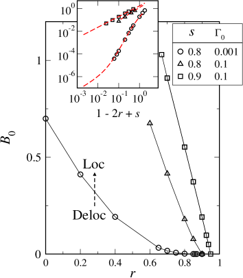
Figure 7: (Color online) Phase diagram in the $r$-$B_{0}$ plane, obtained using NRG for the fixed bosonic bath exponent $s$ and the hybridization strength $\Gamma_{0}$ shown in the legend. For $0<r<r_{+}=(1+s)/2$, we find a continuous QPT between delocalized (Deloc) and localized (Loc) phases. The critical dissipation strength $B_{0,c}$ is found to vanish continuously at $r=r_{+}$. For $r\geq r_{+}$ only the localized phase can be accessed for $B_{0}>0$. The inset shows the vanishing of $B_{0,c}$ with decreasing $1-2r+s$ in each case, compared to the results obtained from the perturbative analysis.

Figure 7 shows the phase diagram of the model on the $r$-$B_{0}$ plane for three different combinations of the bosonic bath exponent $0<s<1$ and the hybridization strength $\Gamma_{0}$. For all $s$ and $\Gamma_{0}$ pairs considered, the phase-boundary value of $B_{0}$ decreases monotonically with increasing $r$ from that found for a metallic conduction band ($r=0$). This is particularly clear from the data set obtained for $s=0.8$ and $\Gamma_{0}=10^{-3}$ (circles in Fig. 7), where the metallic system undergoes a continuous QPT at a critical $B_{0,c}(r=0)\approx 0.699$. With increasing $r$, and hence growing depletion of the conduction electron density of states around the Fermi level, the critical dissipation strength $B_{0,c}$ required to localize the system is reduced, as expected on physical grounds. $B_{0,c}(r)$ is found to vanish continuously at $r=r_{+}$, with $r_{+}$ as defined in Eq. (14). This vanishing is illustrated in the inset to Fig. 7, which shows $B_{0,c}$ vs $1-2r+s$ on a logarithmic scale.

For $r>r_{+}$, localized solutions are found for arbitrarily small dissipation strength $B_{0}>0$. The symbols at the largest $r$ ($=r_{+}$) in each case, which lie at $B_{0}=0$, mark the point at and above which no delocalized solutions can be found with $B_{0}>0$. Thus, we find that we can tune the system to a QPT if, and only if, $0<s\leq 1$ and $0\leq r\leq r_{+}$, in complete agreement with the scenario deduced via the perturbative analyses and illustrated in Fig. 1.

For $0\leq r<1$ and $s=1$, we find a line of Kosterlitz-Thouless-like transitions between delocalized and localized ground states, and for $s>1$ only the delocalized phase is accessed (provided $\Gamma_{0}>0$). For $r>1$ and $s>1$, the essential physics is controlled by the free-impurity fixed point, regardless of the couplings $\Gamma_{0}$ and $B_{0}$.

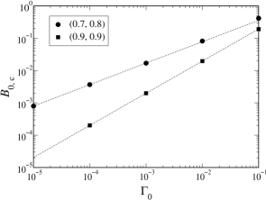
Figure 8: Critical dissipation strength $B_{0,c}$ vs hybridization strength $\Gamma_{0}$ for the $(r,s)$ pairs specified in the legend. We find that $B_{0,c}\propto\Gamma_{0}^{x}$, with $x=(1-s)/(1-r)$.

For a given $(r,s)$ pair that exhibits a continuous QPT, the critical dissipation strength $B_{0,c}$ varies with the hybridization strength $\Gamma_{0}$ as

$$B_{0,c}\propto\Gamma_{0}^{(1-s)/(1-r)}$$ (41)

provided that all scales are small compared to the cutoffs. This result, which follows from dimensional arguments [Eq. (41) can readily be obtained using Eq. (13)] and is confirmed numerically in Fig. 8, identifies $\Gamma_{0}^{1/(1-r)}$ as the tunneling amplitude analogous to $\Delta$ of the spin-boson model, whereBTV the critical dissipation strength is $\alpha_{c}\propto\Delta^{1-s}$. A similar result for the Bose-Fermi Kondo model finds $B_{0,c}\propto T_{K}^{1-s}$, with $T_{K}$ the bare Kondo temperature serving as a tunneling amplitude between impurity spin states.Glossop:05 ; Glossop:07

It is interesting to compare the location of the phase boundary obtained using NRG with that inferred from analytical expansion. We have in mind fixing the hybridization strength $\Gamma_{0}$ and the bosonic-bath exponent $s$ (as in Fig. 7), and finding the critical coupling $B_{0}$ as a function of the conduction-band exponent $r$. However, an analysis of the expansion around the free-impurity fixed point (Sec. II.2) reveals no simple analytical expression for the phase boundary, due to the fact that the problem is described by a two-parameter flow, which cannot be linearized in general. We have therefore analyzed the coupled differential flow equations numerically. The phase boundary can be obtained by determining the eigenvalues and eigenvectors of the linearized RG equations near the critical point and then following the RG flow backwards along the separatrix.

The inset of Fig. 7 compares phase boundaries determined via NRG (symbols) with those obtained via the perturbative RG equations (13) (dashed lines). For the range of $1-2r+s$ considered by NRG, $B_{0,c}$ appears to vanish as a power law, with an exponent that depends on both the bosonic bath exponent $s$ and the hybridization $\Gamma_{0}$. This apparent power law does not reflect the asymptotic behavior, revealed by the perturbative calculations to be $B_{0,c}\propto\tilde{\epsilon}$ as $\tilde{\epsilon}\to 0$. (This regime is inaccessible to NRG because the merging of the critical and delocalized fixed points with decreasing $\tilde{\epsilon}$ make it impossible to reliably determine the critical coupling $B_{0,c}$.) Nevertheless, we find the level of agreement remarkable and stress that there is no fitting procedure involved in making this comparison.

From the expansion around the delocalized fixed point (Sec. II.3), where we have a one-parameter flow, it seems possible to obtain an analytical expression for the phase boundary. However, we have to keep in mind that the dressed $f$ propagator in Eq. (II.3.1) contains terms with different frequency dependencies, and is dominated by $|\omega_{n}|^{r}$ in the low-energy limit only. (The coefficient $A_{1}$ is nonzero in general, except right at the Deloc fixed point.) The interplay of the $|\omega_{n}|^{r}$ and $\omega_{n}$ terms introduces a nonuniversal crossover scale into the problem, and a proper treatment including elevated energies would require a multistage RG scheme, which is beyond the scope of this paper.

III.2 Critical exponents

III.2.1 Correlation-length exponent

The correlation-length exponent $\nu$ defined in Eq. (15) is readily extracted from the crossover scale $T^{*}\propto\Lambda^{-N^{*}/2}$ in the NRG level flows between the unstable and either of the stable fixed points. Here, $N^{*}$ denotes the NRG iteration number at which crossover is observed in a chosen NRG eigenvalue $E_{N}$. (See Refs. Glossop:05, and Glossop:07, for further details.) Figure 9 shows $T^{*}$ vs $|t|=|B_{0}-B_{0,c}|/B_{0,c}$ for the $(r,s)$ pairs specfied in the legend. The dashed lines are linear fits to the log-log data, which yield the correlation length exponent $\nu(r,s)$, independent of the hybridization strength $\Gamma_{0}$ and the phase (Deloc or Loc) from which the QCP is accessed.

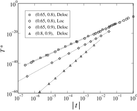
Figure 9: Crossover scale $T^{*}$ vs $|t|=|B_{0}-B_{0,c}|/B_{0,c}$ for the $(r,s)$ pairs specified in the legend. In the vicinity of the transition ($|t|\ll 1$), $T^{*}\propto|t|^{\nu}$. The correlation-length exponent $\nu(r,s)$ is independent both of the hybridization $\Gamma_{0}$ and of the phase from which the QCP is approached.

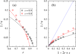
Figure 10: (Color online) (a) Correlation-length exponent $\nu$ vs conduction-band exponent $r$ for two values of the bosonic-bath exponent $s$, as shown in the legend. The symbols show NRG data, while the dashed lines are the corresponding perturbative results [Eq. (16)], expanding about the free-impurity fixed point. We find that $\nu^{-1}$ vanishes at $r=r_{+}$, in keeping with the qualitatively distinct behavior for $2\tilde{\epsilon}\equiv 1-2r+s\gtrless 0$. (b) The same data plotted vs $2\tilde{\epsilon}$. For small $\tilde{\epsilon}$, $\nu^{-1}\approx 2\tilde{\epsilon}$, a result [Eq. (37)] (shown as a dotted line) obtained by a perturbative expansion about the delocalized fixed point.

The $r$ dependence of the correlation-length exponent is demonstrated in Fig. 10(a) for two values of the bosonic bath exponent $s$. As anticipated, for $r=0$ we find that within our estimated numerical error of about 1%, $\nu(0,s)$ is in essentially exact agreement with $\nu(s)$ for the spin-boson modelBTV ; VTB (and the Ising-symmetry Bose-Fermi Kondo model, demonstrated in Ref. Glossop:05, to share the same universality class). By increasing $r$ we find that $\nu(r,s)$ diverges as $r\rightarrow r_{+}$ from below, i.e., as $1-2r+s\to 0^{+}$. The dashed lines are the corresponding perturbative results [Eq. (16)], with which there is excellent agreement for $r$ approaching $r_{+}$. Figure 10(b) shows the same data plotted vs $2\tilde{\epsilon}=1-2r+s$. With decreasing $\tilde{\epsilon}>0$, the curves approach the result $\nu^{-1}\approx 2\tilde{\epsilon}$ (shown as a dotted line), as obtained in Sec. II.C.3 by an expansion about the delocalized fixed point.

III.2.2 Response to a local field

As discussed in Sec. II.2.3, the response to a field applied only at the impurity provides a useful probe of the locally critical properties of the model. The inset to Fig. 11(a) shows $m_{\text{imp}}(t;T=0)$ vs $t=(B_{0}-B_{0,c})/B_{0,c}$ for $(r,s)=(0.85,0.9)$ and hybridization strength $\Gamma=0.1$. Behaving as a suitable order parameter for the problem, $m_{\text{imp}}(t;T=0)$ is finite in the localized phase ($t>0$), saturating to $m_{\text{imp}}(t;T=0)\approx\frac{1}{2}$ for $t\gg 1$ and vanishing continuously as $t\rightarrow 0^{+}$. In the delocalized phase ($t<0$), $m_{\text{imp}}(t;T=0)=0$. The main part of Fig. 11 shows $m_{\text{imp}}(t;T=0)$ vs $t>0$ on a logarithmic scale, from which the power-law behavior Eq. (25) is clearly apparent. The exponent $\beta$ is found to be $\beta=0.601(2)$. At the QCP ($t=0$), the dependence of $m_{\text{imp}}(t=0,T=0)$ on the field $\varepsilon_{f}$ defines the exponent $\delta$ according to Eq. (25). We typically observe such power-law behavior over several orders of magnitude of $\varepsilon_{f}$, as shown in Fig. 11(b). For $(r,s)=(0.85,0.9)$, $1/\delta=0.052(1)$.

We note that for $0\leq r<1$ and $s=1$, $m_{\text{imp}}(t;T=0,\varepsilon_{f}=0^{+})$ undergoes a jump at the critical point $t=0$. Here, the essential behavior has been discussed in Refs. hur1, ; Glossop:05, ; Glossop:07, and Borda:05, for the case $(r,s)=(0,1)$ relevant to charge fluctuations on a metallic island subject to electromagnetic noise.

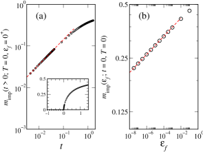
Figure 11: (Color online) Critical exponents $\beta$ and $\delta$, defined in Eq. (25), for $(r,s)=(0.85,0.9)$ and $\Gamma_{0}=0.1$, where $B_{0,c}\approx 0.3731$. (a) Continuous vanishing of order parameter $m_{\text{imp}}$ vs $t=(B_{0}-B_{0,c})/B_{0,c}$ as $t\to 0^{+}$ with characteristic exponent $\beta$ (extracted as the limiting slope of the data on a logarithmic scale). The inset shows the data on an absolute scale. (b) Variation of $m_{\text{imp}}(T=0)$ with local level energy $\varepsilon_{f}$ at the critical point $t=0$. The data clearly follow a power law for small $\varepsilon_{f}$, defining the exponent $\delta$.

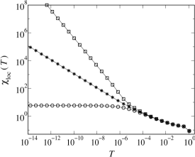
Figure 12: Static local susceptibilty $\chi_{\text{loc}}(T)$ vs $T$ for $(r,s)=(0.2,0.5)$, $\Gamma_{0}=0.1$, and $B_{0}=0.4902$ (circles), $0.5002\approx B_{0,c}$ (stars), and $0.5102$ (squares). The anomalous exponent in the quantum-critical regime is found to be $\eta_{\chi}=1-s$, independent of $r$. See text for further discussion.

We calculate the static local susceptibility via

$$\chi_{\text{loc}}(T)=-\left.\frac{\partial m_{\text{imp}}}{\partial\varepsilon_{f}}\right|_{\varepsilon_{f}=0}=\lim_{\varepsilon_{f}\to 0}-\frac{m_{\text{imp}}}{\varepsilon_{f}}.$$ (42)

In the delocalized phase $B_{0}<B_{0,c}$, $m_{\text{imp}}(T=0)$ vanishes linearly with $\varepsilon_{f}$ and thus $\chi_{\text{loc}}(T)\approx\text{const.}$ for $T\ll T^{*}$. In the localized phase $B_{0}>B_{0,c}$, $m_{\text{imp}}$ is nonzero as $\varepsilon_{f}\to 0$ with $\chi_{\text{loc}}(T\ll T^{*})\propto 1/T$. In the quantum-critical regime $T^{*}\ll T\ll T_{0}$, $\chi_{\text{loc}}(T)$ diverges as a power law with an anomalous exponent $\eta_{\chi}$ defined in Eq. (18). For all $(r,s)$ pairs considered (such that $1-2r+s>0$ and a critical fixed point exists), we find that

$$\eta_{\chi}=1-s\,,$$ (43)

independent of $r$. The behavior described above is clearly illustrated in Fig. 12, which shows three data sets for $(r,s)=(0.2,0.5)$: one at the critical coupling and one close to it in either phase. In this example, we extract $\eta_{\chi}=0.499(2)$.

III.2.3 Hyperscaling

As discussed in Sec. II.2.5, critical exponents for the present model are expected to obey hyperscaling relations derived via a scaling ansatz for the critical part of the free energy that assumes the critical fixed point is interacting.insi This expectation is borne out by the numerical analysis: we find hyperscaling relations to be obeyed to within the estimated error (typically less than 1%) across the range of $(r,s)$ displaying critical behavior. For example, for the case $(r,s)=(0.85,0.9)$, $1/\nu=0.082(1)$ and $\eta_{\chi}=0.101(2)$. Thus, the values $\beta=0.601(2)$ and $1/\delta=0.052(1)$ extracted from the data presented in Fig. 11 obey Eqs. (25) to within numerical uncertainty.

III.3 Spectral function

We now turn to the single-particle spectral function $A(\omega)$, calculated via

$$A(\omega)=\sum_{n,m}\left|\langle n|f^{\dagger}|m\rangle\right|^{2}\frac{e^{-\beta E_{m}}\!+\!e^{-\beta E_{n}}}{Z}\,\delta(\omega-E_{n}+E_{m}),$$ (44)

where $|m\rangle$ is a many-body eigenstate of NRG iteration $N$, and $Z=\sum_{n}\exp(-\beta E_{n})$ is the partition function; $A(\omega)=A(-\omega)$ for the p-h symmetric parameters studied. The discrete delta-functions are Gaussian broadened on a logarithmic scale: a standard NRG procedure discussed, e.g., in Ref. Bulla:07, . We set the broadening parameter $b$ such that $A(\omega)$ for the simplest resonant-level model (with $r=0$, $B_{0}=0$, and $\varepsilon_{f}=0$) is in optimal agreement with the exact result $A(\omega)=\pi^{-1}\Gamma_{0}/(\omega^{2}+\Gamma_{0}^{2})$.

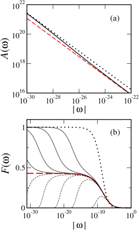
Figure 13: (Color online) (a) Spectral function $A(\omega)$ vs $|\omega|$ for $r=0.65$, $s=0.8$, $\Gamma_{0}=10^{-3}$, and three values of the dissipation strength: $B_{0}=0$ (dotted line), $B_{0}=B_{0,c}-10^{-5}$ (solid line), and $B_{0}=B_{0,c}=0.03247113$ (thick dashed line). At the quantum critical point $B_{0}=B_{0,c}$, $A(\omega)\propto|\omega|^{-r}$, which behavior is also followed for $B_{0}$ close to $B_{0,c}$ and $|\omega|\gg T_{*}$. In the delocalized phase $B_{0}<B_{0,c}$, there is a crossover in $A(\omega)$ to the behavior Eq. (45) for $|\omega|\ll T_{*}$. For the data shown, $T^{*}\sim\mathcal{O}(10^{-26})$. (b) The crossover behavior is more readily seen in the modified spectral function $\mathcal{F}(\omega)=\pi\Gamma_{0}\sec^{2}(\frac{\pi}{2}r)|\omega|^{r}A(\omega)$, which shows the ultimate low-$\omega$ behavior $\mathcal{F}(\omega=0)=1$ throughout the delocalized phase $B_{0}<B_{0,c}$, $0<\mathcal{F}(\omega=0)<1$ for $B_{0}=B_{0,c}$, and $\mathcal{F}(\omega=0)=0$ throughout the localized phase $B_{0}>B_{0,c}$. In order of decreasing crossover scale, delocalized-phase spectra are shown for $B_{0}=0$ (dotted line) and for $B_{0,c}-B_{0}=$ $10^{-3}$, $10^{-4}$, $10^{-5}$, and $10^{-6}$ (solid lines); localized-phase spectra (dashed lines) are shown for $B_{0}=0.05$ and $B_{0}-B_{0,c}=$ $10^{-3}$, $10^{-4}$, $10^{-5}$, and $10^{-6}$. The critical spectrum is shown as a thick dashed line.

Figure 13(a) shows $A(\omega)$ vs $|\omega|$ on a logarithmic scale for $r=0.65$, $s=0.8$, $\Gamma_{0}=10^{-3}$, and the dissipation strengths $B_{0}\leq B_{0,c}$ specified in the figure caption. For the delocalized phase $B_{0}<B_{0,c}$, we find that the dissipation does not alter the asymptotic low-frequency behavior of $A(\omega)$ found for $B_{0}=0$, i.e.,

$$A(\omega)=\frac{1}{\pi\Gamma_{0}}\,\cos^{2}\!\!\left(\frac{\pi r}{2}\right)|\omega|^{-r}\ \ \ \text{for }|\omega|\ll T^{*}.$$ (45)

For $B_{0}=0$ the spectrum is identical to that obtained for the noninteracting ($U=0$) limit of the (spinful) pseudogap Anderson model at p-h symmetry, where the result Eq. (45) holds for $0<r<1$.GBI Moreover, it is knownLogan:00 ; Bulla:00 that the form Eq. (45) persists throughout the Kondo-screened phase of the pseudogap Anderson model with interactions present (i.e., for all $U<U_{c}$), which in the p-h symmetric case is confined to $0<r<\mbox{$\frac{1}{2}$}$.

In the vicinity of the QCP, $B_{0}\approx B_{0,c}$, we find

$$A(\omega)=\frac{\tilde{c}(r,s)}{\pi\Gamma_{0}}\,\cos^{2}\!\!\left(\frac{\pi r}{2}\right)|\omega|^{-r}\ \ \ \text{for }T^{*}\ll|\omega|\ll T_{0},$$ (46)

where $\tilde{c}(r,s)\leq 1$ and $T_{0}$ is a high-frequency cutoff set by the bare hybridization strength $\Gamma_{0}$. This behavior confirms Eqs. (22) and (23).

In the localized phase, by contrast, $A(\omega)$ vanishes as $\omega\to 0$:

$$A(\omega)\propto|\omega|^{a}\ \ \ \text{for }|\omega|\ll T^{*}.$$ (47)

The exponent $a$ is positive, and in general depends on both $r$ and $s$.

The crossover between these behaviors is more readily apparent in the modified spectral function $\mathcal{F}(\omega)=\pi\Gamma_{0}\sec^{2}(\pi r/2)|\omega|^{r}A(\omega)$. Any low-frequency divergence of $A(\omega)$ is canceled in $\mathcal{F}(\omega)$, and $\mathcal{F}(0)=1$ is pinned throughout the delocalized phase of the model. As discussed in the context of the pseudogap Anderson model,Glossop:00 ; Logan:00 ; Bulla:00 this generalizes the well-known pinning $\pi\Gamma_{0}A(0)=1$ of the spectral function for the regular ($r=0$, fermionic) Anderson model. In the delocalized phase, the scale $T^{*}$, playing the role of a renormalized tunneling amplitude, is then manifest as the width of the pinned resonance at the Fermi level $\omega=0$, vanishing as $B_{0}\to B_{0,c}^{-}$.

Figure 13(b) shows $\mathcal{F}(\omega)$ vs $|\omega|$ for $r=0.65$, $s=0.8$, $\Gamma_{0}=10^{-3}$, and the $B_{0}$ values specified in the figure caption. Throughout the delocalized phase ($0\leq B_{0}<B_{0,c}$), $\mathcal{F}(0)=1$ remains satisfied to within a few percent, as is typical for NRG. Close to the QCP in either phase, $\mathcal{F}(\omega)\approx\tilde{c}(r,s)$ down to the scale $T^{*}$.

We close by considering the single-particle spectrum for the case of a metallic fermionic density of states ($r=0$) and Ohmic dissipation ($s=1$). Here the model describes charge fluctuations on a quantum dot or resonant tunneling device close to a degeneracy point and subject to electromagnetic noise. The essential physics—a Kosterlitz-Thouless-like QPT between delocalized and localized states—has been investigated in a number of earlier studies hur1 ; Borda:05 ; hur2 ; zarand ; Glossop:07 , e.g., via a Bose-Fermi Kondo model, and we will not repeat the discussion here. We simply show, in Fig. 14, the spectrum for $\Gamma_{0}=0.001$ and a range of dissipation strengths; for $B_{0}=0$, $A(\omega)$ is of Lorentzian form. The vanishing width of the central resonance as $B_{0}\to B_{0,c}^{-}$ indicates a suppression of tunneling between dot and leads due to the noisy electromagnetic environment.

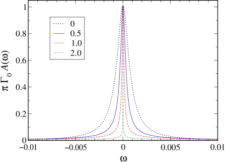
Figure 14: (Color online) $\pi\Gamma_{0}A(\omega)$ vs $\omega$ for the case of a metallic fermionic density of states ($r=0$) and Ohmic dissipation ($s=1$) for $\Gamma_{0}=0.001$. Spectra are shown for increasing dissipation strength $B_{0}$ (see legend) in the delocalized phase. The spectrum is a simple Lorentzian for $B_{0}=0$, and the vanishing width as $B_{0}\to B_{0,c}^{-}$ indicates a suppression of tunneling between the local level and the conduction band.

IV Conclusions

In this paper, we have analyzed the phase diagram and the quantum phase transitions of a paradigmatic quantum impurity model with both fermionic and bosonic baths, namely a dissipative resonant-level model. For weak dissipation, the resonant tunneling of electrons is renormalized due to the friction of the bosonic bath, but the ground state remains delocalized. For strong dissipation, by contrast, the tunneling amplitude renormalizes to zero in the low-energy limit leading to a localized ground state. We have employed both analytical and numerical techniques, utilizing epsilon expansions recently developed in the context of the pseudogap Anderson and Kondo model, and an extension of Wilson’s numerical renormalization-group approach, generalized to treat both fermionic and bosonic baths.

The transition between delocalized and localized phases exists for a wide range of exponents $r$ and $s$ characterizing the conduction-band and bosonic-bath densities of states, respectively. Our epsilon expansions, formulated in the original degrees of freedom, are in excellent agreement with numerics in the vicinity of the expansion points. For the case of a metallic bath, inaccessible to the analytical techniques used here, we have presented numerical results, making contact with earlier bosonization studies of related models.

We finally mention a few applications. In the context of nanostructures, a resonant-level model may describe the tunneling of electrons between a lead and a small island or quantum dot.matveev ; berman Taking into account electromagnetic noise of a fluctuating environment directly leads to a model of type (I), provided that the spin degree of freedom of the electrons can be neglected (e.g., if electrons are spin-polarized due to a large applied magnetic field). Related situations, mainly corresponding to bath exponents $r=0$ and $s=1$, have been discussed in the literature.hur1 ; hur2 Apart from the common situation of ohmic noise ($s=1$), sub-ohmic dissipation ($s<1$) can occur, e.g., in RLC transmission lines which display a $\sqrt{\omega}$ spectrum in the R-dominant limit.nazarov Further, a bath with $r=1$ may be realized using Dirac electrons of graphene or quasiparticles of a $d$-wave superconductor.

- (1) S. Sachdev, Quantum Phase Transitions (Cambridge University Press, Cambridge, 1999).
- (2) M. Vojta, Philos. Mag. 86, 1807 (2006).
- (3) A. Georges, G. Kotliar, W. Krauth, and M. J. Rozenberg, Rev. Mod. Phys. 68, 13 (1996).
- (4) Q. Si, S. Rabello, K. Ingersent, and J. L. Smith, Nature (London) 413, 804 (2001); Phys. Rev. B68, 115103 (2003).
- (5) R. M. Potok, I. G. Rau, H. Shtrikman, Y. Oreg, and D. Goldhaber-Gordon, Nature (London) 446, 167 (2007).
- (6) L. G. G. V. Dias da Silva, N. P. Sandler, K. Ingersent, and S. E. Ulloa, Phys. Rev. Lett. 97, 096603 (2006).
- (7) L. Kouwenhoven and L. Glazman, Physics World 14, 33 (2001); D. Goldhaber-Gordon et al., Nature 391, 156 (1998); W. G. van der Wiel et al., Science 289, 2105 (2000); L. I. Glazman and M. E. Raikh, Sov. Phys. JETP Lett. 47, 452 (1988).
- (8) D. P. DiVincenzo et al., in Quantum Mesoscopic Phenomena and Mesoscopic Devices in Microelectronics, edited by O. Kulik and R. Ellialtoglu (NATO, Turkey, 1999).
- (9) K. A. Matveev, Zh. Eksp. Thor. Fiz. 99, 1598 (1991) [Sov. Phys. JETP 72, 892 (1991)]; P. Cedraschi et al., Phys. Rev. Lett. 91, 106801 (2003); P. Cedraschi and M. Büttiker, Annals of Physics 289, 1 (2001).
- (10) D. Withoff and E. Fradkin, Phys. Rev. Lett. 64, 1835 (1990).
- (11) C. R. Cassanello and E. Fradkin, Phys. Rev. B 53, 15079 (1996); ibid. 56, 11246 (1997).
- (12) C. Gonzalez-Buxton and K. Ingersent, Phys. Rev. B57, 14254 (1998).
- (13) K. Ingersent and Q. Si, Phys. Rev. Lett. 89, 076403 (2002).
- (14) M. Vojta and L. Fritz, Phys. Rev. B 70, 094502 (2004).
- (15) L. Fritz and M. Vojta, Phys. Rev. B 70, 214427 (2004).
- (16) R. Bulla, N. Tong, and M. Vojta, Phys. Rev. Lett. 91, 170601 (2003).
- (17) R. Bulla, H.-J. Lee, N.-H. Tong, and M. Vojta, Phys. Rev. B71, 045122 (2005).
- (18) R. Bulla, T. Costi, and T. Pruschke, cond-mat/0701105.
- (19) A. J. Leggett, S. Chakravarty, A. T. Dorsey, M. P. A. Fisher, A. Garg, and W. Zwerger, Rev. Mod. Phys. 59, 1 (1987).
- (20) M. Vojta, N. Tong, and R. Bulla, Phys. Rev. Lett. 94, 070604 (2005).
- (21) Q. Si and J. L. Smith, Phys. Rev. Lett. 77, 3391 (1996); J. L. Smith and Q. Si, Phys. Rev. B 61, 5184 (2000).
- (22) R. Chitra and G. Kotliar, Phys. Rev. Lett. 84, 3678 (2000).
- (23) J. L. Smith and Q. Si, cond-mat/9705140; Europhys. Lett. 45, 228 (1999).
- (24) A. M. Sengupta, Phys. Rev. B 61, 4041 (2000).
- (25) L. Zhu and Q. Si, Phys. Rev. B 66, 024426 (2002); G. Zarand and E. Demler, Phys. Rev. B 66, 024427 (2002).
- (26) M. Vojta and M. Kirćan, Phys. Rev. Lett. 90, 157203 (2003).
- (27) S. Kirchner, L. Zhu, Q. Si, and D. Natelson, Proc. Natl. Acad. Sci. USA 102, 18824 (2005).
- (28) M. T. Glossop and K. Ingersent, Phys. Rev. Lett. 95, 67202 (2005).
- (29) M. T. Glossop and K. Ingersent, Phys. Rev. B 75, 104410 (2007).
- (30) K. Le Hur, Phys. Rev. Lett 92, 196804 (2004).
- (31) Note that in the spinful p-h symmetric Anderson model, a local interaction term will render the resonant-level fixed point at unstable for (driving the system into the local-moment regime); see Ref. larslong, .
- (32) E. Brezin, J. C. Le Guillou, and J. Zinn-Justin, in Phase transitions and critical phenomena, Vol. 6, edited by C. Domb and M. S. Green (Page Bros., Norwich, 1996).
- (33) R. Bulla, T. Pruschke, and A. C. Hewson, J. Phys. Condens. Matter 9, 10463 (1997).
- (34) M. T. Glossop and D. E. Logan, Eur. Phys. J. B 13, 513 (2000).
- (35) D. E. Logan and M. T. Glossop, J. Phys. Condens. Matter 12, 985 (2000).
- (36) R. Bulla, M. T. Glossop, D. E. Logan, and T. Pruschke, J. Phys. Condens. Matter 12, 4899 (2000).
- (37) L. Borda, G. Zaránd, and P. Simon, Phys. Rev. B 72, 155311 (2005).
- (38) L. Borda, G. Zarand, and D. Goldhaber-Gordon, cond-mat/0602019.
- (39) M.-R. Li, K. Le Hur, and W. Hofstetter, Phys. Rev. Lett. 95, 086406 (2005), K. Le Hur and M.-R. Li, Phys. Rev. B 72, 073305 (2005).
- (40) A. Furusaki and K. A. Matveev, Phys. Rev. Lett. 88, 226404 (2002).
- (41) G.-L. Ingold and Y. V. Nazarov, “Single charge tunneling Coulomb Blockade phenomena in nanostructures”, Chap. 2, NATO ASI Series, Series B: Physics, Vol. 294, edited by H. Grabert and M. H. Devoret (Plenum Press, New York, 1992).
- (42) D. Berman, N. B. Zhitenev, R. C. Ashoori, and M. Shayegan, Phys. Rev. Lett. 82, 161 (1999).