Neutrino Masses and Lepton-flavor-violating $\tau$ Decays in the Supersymmetric Left-right Model

Abstract

In the supersymmetric left-right model, the light neutrino masses are given by the Type-II seesaw mechanism. A duality property about this mechanism indicates that there exist eight possible Higgs triplet Yukawa couplings which result in the same neutrino mass matrix. In this paper, We work out the one-loop renormalization group equations for the effective neutrino mass matrix in the supersymmetric left-right model. The stability of the Type-II seesaw scenario is briefly discussed. We also study the lepton-flavor-violating processes ( $\tau\rightarrow\mu\gamma$ and $\tau\rightarrow e\gamma$ ) by using the reconstructed Higgs triplet Yukawa couplings.

I introduction

Current solar, atmospheric, reactor and accelerator neutrino oscillation experiments have provided us with very convincing evidence that neutrinos have non-vanishing masses and lepton flavors are mixed[1, 2, 3, 4, 5]. A global analysis of current experimental data yields $30^{\circ}\leq\theta_{12}\leq 38^{\circ}$, $36^{\circ}\leq\theta_{23}\leq 54^{\circ}$ and $0<\theta_{13}<10^{\circ}$ as well as $\Delta m^{2}_{21}\equiv m^{2}_{2}-m^{2}_{1}=(7.2\cdot\cdot\cdot 8.9)\times 10^{-5}~{}{\rm eV}^{2}$ and $\Delta m^{2}_{32}\equiv m^{2}_{3}-m^{2}_{2}=\pm(2.1\cdot\cdot\cdot 3.1)\times 10^{-3}~{}{\rm eV}^{2}$ at the $99\%$ confidence level[6], but three CP-violating phases (i.e., the Dirac phase $\delta$ and the Majorana phases $\rho$ and $\sigma$ ) are entirely unrestricted. These important results indicate that there should be a more fundamental theory beyond the standard model, in which three neutrinos are massless Weyl particles. One possible candidate for such a theory is the supersymmetric version of the left-right symmetric model[7], which provides a natural embedding of the seesaw mechanism for small neutrino masses[8].

The supersymmetric left-right model[9, 10] is based on the gauge group $SU(3)_{C}\times SU(2)_{L}\times SU(2)_{R}\times U(1)_{B-L}$. The quarks and leptons transform under the gauge group as $Q(3,2,1,1/3)$, $Q^{c}(3^{*},1,2,-1/3)$, $L(1,2,1,-1)$ and $L^{c}(1,1,2,1)$. In the gauge sector, there are triplet gauge bosons $(W^{+},W^{-},W^{0})_{L}$, $(W^{+},W^{-},W^{0})_{R}$ corresponding to $SU(2)_{L}$ and $SU(2)_{R}$ and a vector boson $V$ corresponding to $U(1)_{B-L}$, together with their superpartners. Fermion masses arise from the Yukawa coupling between quarks, leptons and Higgs bi-doublets: $\Phi_{u}(2,2,0)$ and $\Phi_{d}(2,2,0)$. The gauge group $SU(2)_{R}\times U(1)_{B-L}$ is broken to the hypercharge symmetry $U(1)_{Y}$ by the vacuum expectation value (vev) of a $B-L=-2$ Higgs triplet $\Delta^{c}(1,1,3,-2)$ which is accompanied by a left-handed Higgs triplet $\Delta(1,3,1,2)$. The choice of the triplets is preferred because with this choice the seesaw arises from purely renormalizable interactions. In addition to $\Delta\ {\rm and}\ \Delta^{c}$, the model must contain their conjugate fields $\bar{\Delta}\ {\rm and}\ \bar{\Delta}^{c}$ to insure the cancellation of the anomalies that would otherwise occur in the fermionic sector. Given their strange quantum numbers, the $\bar{\Delta}$ and $\bar{\Delta}^{c}$ do not couple to any of the particles in the theory, and thus their contributions are negligible for any phenomenological studies. The gauge invariant part of the matter superpotential can be written as

$$W=Y_{q}^{i}(Q^{c})^{T}\tilde{\Phi}_{i}Q+Y_{l}^{i}(L^{c})^{T}\tilde{\Phi}_{i}L+i\left({\cal F}L^{T}\tau_{2}\Delta L+{\cal F}_{c}{L^{c}}^{T}\tau_{2}\Delta^{c}L^{c}\right),$$ (1)

where $\tilde{\Phi}_{i}=i\tau_{2}\Phi_{i}$ is defined and $i=u,d$. All the couplings $Y_{q}^{i}$, $Y_{l}^{i}$, ${\cal F}$ and ${\cal F}_{c}$ are complex with ${\cal F}$ and ${\cal F}_{c}$ being symmetric matrices. The left-right symmetry implies $Y_{\alpha}^{i}=(Y_{\alpha}^{i})^{\dagger}$ $(\alpha=q,l)$ and ${\cal F}={\cal F}_{c}^{*}$. Given the vevs of $\Phi_{u,d}$, $\Delta$ and $\Delta^{c}$,

$$\langle\Phi_{u}\rangle = \left(\matrix{\kappa_{u}&0\cr 0&0\cr}\right),\hskip 42.67912pt\langle\Phi_{d}\rangle=\left(\matrix{0&0\cr 0&\kappa_{d}\cr}\right),$$ (2)

$$\langle\Delta\rangle = \left(\matrix{0&0\cr v_{L}&0\cr}\right),\hskip 42.67912pt\langle\Delta^{c}\rangle=\left(\matrix{0&0\cr v_{R}&0\cr}\right),$$ (3)

the gauge group is broken to $U(1)_{em}$ and the up-type quark, down-type quark, charged lepton and Dirac neutrino mass matrices turn out to be: $M_{u}=Y_{q}^{u}\kappa_{u}$, $M_{d}=Y_{q}^{d}\kappa_{d}$, $M_{l}=Y_{l}^{u}\kappa_{d}$ and $M_{D}=Y_{l}^{d}\kappa_{u}$. Meanwhile, the left- and right-handed Majorana neutrino mass matrices can be obtained from the corresponding mass terms in Eq. (1) once the Higgs triplets $\Delta$ and $\Delta^{c}$ acquire their vevs: $M_{L}\simeq v_{L}{\cal F}$ and $M_{R}\simeq v_{R}{\cal F}$. Integrating out the heavy particles (i.e., the right-handed Majorana neutrinos and Higgs triplet), one obtains the effective mass matrix for three light (left-handed) Majorana neutrinos via the Type-II seesaw mechanism[11]:

$$M_{\nu}\;\simeq\;M_{L}-M_{D}^{T}M_{R}^{-1}M_{D}\;\simeq\;v_{L}{\cal F}-{1\over v_{R}}M_{D}^{T}{\cal F}^{-1}M_{D}\;.$$ (4)

We may find that the same coupling ${\cal F}$ appears in both contributions just because of the left-right symmetry.

Note that Eq. (3) has a duality property[12]: given $M_{D}$, there exist eight possible Higgs triplet Yukawa couplings which result in the same neutrino mass matrix. The stability of the duality relation and some other phenomena based on this have been investigated recently. In this paper we perform a full analysis of the renormalization group equations (RGEs) of the effective neutrino mass operators. We write down the $\beta$-functions of the effective neutrino mass operators and discuss the stability of the Type-II seesaw mechanism. Lepton-flavor-violating decays in the supersymmetric left-right model are different from that in the minimal supersymmetric standard model (MSSM) for the existence of the Higgs triplet Yukawa coupling ${\cal F}$[13, 25]. In this paper, we calculate the ${\rm BR}(\tau\rightarrow\mu\gamma)$ and ${\rm BR}(\tau\rightarrow e\gamma)$ by using the reconstructed Higgs triplet Yukawa couplings in the supersymmetric left-right model.

The remaining part of this paper is organized as follows. In section II, we calculate the one-loop RGEs for the effective neutrino mass operators. Section III is devoted to studying the lepton-flavor-violating processes. A summary of our main results is given in section IV. Some useful formulas are listed in appendices A and B.

II renormalization group equations of the effective neutrino mass operators

We assume that the gauge and discrete left-right symmetries are both broken by the vev of $\Delta^{c}$ at the high energy scale in our model. As a result the right-handed neutrinos and Higgs triplets are much heavier than other particles. Integrating out the right-handed neutrinos in the leading-order approximation, one obtains the effective neutrino mass operators, which are contained in the $F$-term of the superpotential,

$${\cal W}_{\kappa} = -{1\over 4}(\kappa_{\rm 1})_{gf}l^{g}_{c}\varepsilon^{ce}(\Phi_{u})_{e1}l^{g}_{a}\varepsilon^{ab}(\Phi_{u})_{b1}-{1\over 4}(\kappa_{\rm 2})_{gf}l^{f}_{c}\varepsilon^{ce}(\Phi_{d})_{e1}l^{f}_{a}\varepsilon^{ab}(\Phi_{d})_{b1}$$ (6)

$$-{1\over 4}(\kappa_{\rm 3})_{gf}l^{g}_{c}\varepsilon^{ce}(\Phi_{u})_{e1}l^{f}_{a}\varepsilon^{ab}(\Phi_{d})_{b1}+{\rm h.c.},$$

where

$$\kappa_{\rm 1} = 2\left[(Y_{l}^{u})^{T}(v_{R}{\cal F})^{-1}Y_{l}^{u}\right],$$ (7)

$$\kappa_{\rm 2} = 2\left[(Y_{l}^{d})^{T}(v_{R}{\cal F})^{-1}Y_{l}^{d}\right],$$ (8)

$$\kappa_{\rm 3} = \left[(Y_{l}^{u})^{T}(v_{R}{\cal F})^{-1}Y_{l}^{d}+(Y_{l}^{d})^{T}(v_{R}{\cal F})^{-1}Y_{l}^{u}\right].$$ (9)

Due to the non-renormalization theorem[14], the RGEs for operators of the superpotential are governed by the wave function renormalization for the superfields. At the one-loop level the wave-function renormalizaton constants $Z$ are obtained with the dimensional regularization via the dimensional reduction[15]:

$$-(4\pi)^{2}\delta Z_{\Phi_{u}} = 6{\rm Tr}\left[(Y_{q}^{u})^{\dagger}Y_{q}^{u}\right]+2{\rm Tr}\left[(Y_{l}^{u})^{\dagger}Y_{l}^{u}\right]-{3\over 5}g_{1}^{2}-3g_{2}^{2}\ ,$$ (10)

$$-(4\pi)^{2}\delta Z_{\Phi_{d}} = 6{\rm Tr}\left[(Y_{q}^{d})^{\dagger}Y_{q}^{d}\right]+2{\rm Tr}\left[(Y_{l}^{d})^{\dagger}Y_{l}^{d}\right]-{3\over 5}g_{1}^{2}-3g_{2}^{2}\ ,$$ (11)

$$-(4\pi)^{2}\delta Z_{l\ \ } = 2\left[(Y_{l}^{u})^{\dagger}Y_{l}^{u}+\ (Y_{l}^{d})^{\dagger}Y_{l}^{d}+\ {\cal F}{\cal F^{\dagger}}\right]-{3\over 5}g_{1}^{2}-3g_{2}^{2}\ ,$$ (12)

$$-(4\pi)^{2}\delta Z_{\Delta\ } = 4{\rm Tr}\left[{\cal F}{\cal F^{\dagger}}\right]-{12\over 5}g_{1}^{2}-8g_{2}^{2}\ .$$ (13)

Using the counterterms calculated above and the technique described in Ref. [16], we obtain the $\beta$-functions ($\beta_{X}\equiv\mu{d\over d\mu}X$) of the effective mass operators $\kappa_{i}$ $(i=1,2,3)$ and the Higgs triplet Yukawa coupling ${\cal F}$ :

$$16\pi^{2}\beta_{\kappa_{1}} = {\cal R}^{T}\cdot\kappa_{1}+\kappa_{1}\cdot{\cal R}+\left\{6{\rm Tr}\left[(Y_{q}^{u})^{\dagger}Y_{q}^{u}\right]-{6\over 5}g_{1}^{2}-6g_{2}^{2}\right\}\kappa_{1}\ ,$$ (14)

$$16\pi^{2}\beta_{\kappa_{2}} = {\cal R}^{T}\cdot\kappa_{2}+\kappa_{2}\cdot{\cal R}+\left\{6{\rm Tr}\left[(Y_{q}^{d})^{\dagger}Y_{q}^{d}\right]-{6\over 5}g_{1}^{2}-6g_{2}^{2}\right\}\kappa_{2}\ ,$$ (15)

$$16\pi^{2}\beta_{\kappa_{3}} = {\cal R}^{T}\cdot\kappa_{3}+\kappa_{3}\cdot{\cal R}+\left\{3{\rm Tr}\left[(Y_{q}^{u})^{\dagger}Y_{q}^{u}\right]+3{\rm Tr}\left[(Y_{q}^{d})^{\dagger}Y_{q}^{d}\right]-{6\over 5}g_{1}^{2}-6g_{2}^{2}\right\}\kappa_{3}\ ,$$ (16)

$$16\pi^{2}\beta_{\cal F}\ = {\cal R}^{T}\cdot{\cal F}+\ {\cal F}\cdot{\cal R}+\left\{2{\rm Tr}\left[{\cal F}{\cal F^{\dagger}}\right]-{9\over 5}g_{1}^{2}-7g_{2}^{2}\right\}{\cal F},$$ (17)

where

$${\cal R}\equiv(Y_{l}^{u})^{\dagger}Y_{l}^{u}+(Y_{l}^{d})^{\dagger}Y_{l}^{d}+{\cal F}{\cal F^{\dagger}}.$$ (18)

Some comments are in order.

• In calculating the $\beta$-functions, we have assumed $M_{\Delta}$ (the mass of the Higgs triplet) to be lighter than $M_{1}$ which is the mass of the lightest right-handed neutrinos. Actually this assumption is not necessary. One may integrate out $\nu_{R}$ and $\Delta$ each at its own mass scale and redefining iteratively the effective operator, which is more reasonable. Below $m_{\Delta}$, the $\beta$-functions of the effective mass operators, which come from integrating out the Higgs triplet, are similar to $\kappa_{i}$’s.

• Given the vacuum expectation values of the Higgs bi-doublets and triplets in Eq. (2), only $\kappa_{1}$ gives rise to masses of the light left-handed neutrinos after spontaneous electro-weak symmetry breaking. We just need to calculate the $\beta$-function of $\kappa_{1}$ when considering the renormalization group effects of neutrino mass operators. Besides, all operators in ${\cal W}_{\kappa}$ contribute to the lepton-flavor-violating processes. However, such processes are strongly suppressed by heavy masses of the right-handed neutrinos.

• Below the lightest seesaw scale, the $\beta$-function of the effective neutrino mass operator prossess the same as that of the Type-I seesaw model in the MSSM, only up to a replacement $Y_{l}^{\dagger}Y_{l}$ $\longrightarrow$ $(Y_{l}^{u})^{\dagger}Y_{l}^{u}+(Y_{l}^{d})^{\dagger}Y_{l}^{d}$.

Due to the renormalization group (RG) evolution effects between the $M_{\Delta}$ and $M_{1}$ scales, the seesaw formula in Eq. (3) is modified, where two ${\cal F}$’s in Type-I and Type-II terms are not equal anymore. As a result the duality property is slightly broken when considering the RG evolution effects of ${\cal F}$ and the effective neutrino mass operator.

III Lepton Flavor Violation in the Supersymmetric Left-Right Model

In this section, we first give the analytical formulas to be used for the calculation of the lepton-flavor-violating processes and then list our numerical results.

A Analytical formulas

Working in the basis where the sleptons are in weak eigenstates together with the charginos (neutralinos) in their mass eigenstates, we write down the interaction Lagrangian of lepton-slepton-chargino in the following form:

$$-{\cal L}_{int} = +{\tilde{\nu}}^{\dagger}_{Li}\overline{{\tilde{\chi}}^{-}_{A}}(C^{A(i)}_{LR}P_{R}+C_{LL}^{A(i)}P_{L})l_{i}+{\tilde{\nu}}^{\dagger}_{Ri}\overline{{\tilde{\chi}}^{-}_{A}}(C^{A(i)}_{RR}P_{R}+C_{RL}^{A(i)}P_{L})l_{i}$$ (21)

$$+{\tilde{e}}^{\dagger}_{Li}\overline{\tilde{\chi}^{0}_{A}}(N^{A(i)}_{LR}P_{R}+N_{LL}^{A(i)}P_{L})l_{i}+{\tilde{e}}^{\dagger}_{Ri}\overline{\tilde{\chi}^{0}_{A}}(N^{A(i)}_{RR}P_{R}+N_{RL}^{A(i)}P_{L})l_{i}$$

$$+{\rm h.c.},$$

where the coefficients are:

$$C_{LL}^{A(i)} = g_{L}({\cal O}_{R})_{A1},$$ (22)

$$C_{LR}^{A(i)} = -{g_{L}m_{ei}\over\sqrt{2}m_{W}\cos\beta}({\cal O}_{L})_{A3}+{g_{L}m^{D}_{\nu i}\over\sqrt{2}m_{W}\sin\beta}({\cal O}_{L})_{A4},$$ (23)

$$C_{RR}^{A(i)} = g_{R}({{\cal O}_{L}})_{A2},$$ (24)

$$C_{LR}^{A(i)} = -{g_{L}m_{ei}\over\sqrt{2}m_{W}\cos\beta}({\cal O}_{R})_{A3}+{g_{L}m^{D}_{\nu i}\over\sqrt{2}m_{W}\sin\beta}({\cal O}_{R})_{A4},$$ (25)

$$N_{LL}^{A(i)} = {g_{L}\over\sqrt{2}}\left[-({{\cal O}_{N}})_{A2}-({{\cal O}_{N}})_{A1}\tan\theta_{W}\right],$$ (26)

$$N_{LR}^{A(i)} = {g_{L}m_{ei}\over\sqrt{2}m_{W}\cos\beta}\left[({{\cal O}_{N}})_{A3}-({{\cal O}_{N}})_{A4}\right]+{g_{L}m^{D}_{\nu i}\over\sqrt{2}m_{W}\sin\beta}\left[({{\cal O}_{N}})_{A6}-({{\cal O}_{N}})_{A5}\right],$$ (27)

$$N_{RL}^{A(i)} = N_{LR}^{A(i)},$$ (28)

$$N_{RR}^{A(i)} = {g_{R}\over\sqrt{2}}\left[-({{\cal O}_{N}})_{A7}-({{\cal O}_{N}})_{A1}\tan\theta_{W}\right].$$ (29)

Here ${\cal O}_{L}$, ${\cal O}_{R}$ and ${\cal O}_{N}$ are real orthogonal matrices that diagonalize chargino and neutralino mass matrices respectively. Their explicit forms are listed in appendix A. $\tan\beta\equiv\kappa_{u}/\kappa_{d}$ is defined.

Let us discuss the branching ratios of the lepton-flavor-violating processes in the supersymmetric left-right model. The radiative decays $l_{i}\rightarrow l_{j}+\gamma$ are induced by the effective operator[17]:

$$e\overline{l_{j}}\left(iD_{L}^{\gamma}P_{L}+iD_{R}^{\gamma}P_{R}\right)\sigma^{\mu\nu}l_{i}F_{\mu\nu}+{\rm h.c.}\ ,$$ (30)

where $e$ and $F_{\rho\sigma}$ are the charge and the electromagnetic field strength, respectively. These operators are chirality-flipping (dipole) and come from $SU(2)_{\rm L}\times U(1)_{\rm Y}$-invariant operators with at least one Higgs field.

In the “mass insertion” method and leading-log approximations, the coefficients $D^{\gamma}_{L,R}$ can be calculated[13] and we write down the explicit expression in appendix A. The branching ratio of $l_{i}\rightarrow l_{j}+\gamma$ decay due to the new contributions is given by:

$${\rm BR}(l_{i}\rightarrow l_{j}\gamma)={48\pi^{3}\alpha\over m_{l_{i}}^{2}G_{F}^{2}}\left(\mid D_{L}^{\gamma}\mid^{2}+\mid D_{R}^{\gamma}\mid^{2}\right){\rm BR}(l_{i}\longrightarrow l_{j}\bar{\nu}_{j}\nu_{i}),$$ (31)

where $\alpha=e^{2}/(4\pi)$, $G_{F}$ is the Fermi constant, ${\rm BR}(\tau\rightarrow\mu\nu_{\tau}\overline{\nu}_{\mu})\approx 17\%$ and ${\rm BR}(\tau\rightarrow e\nu_{\tau}\overline{\nu}_{e})\approx 18\%$[18].

In the minimal SUGRA scenario, at the gravitational scale the supersymmetry breaking masses for sleptons, squarks and the Higgs bosons are universal, and the SUSY breaking parameters associated with the supersymmetric Yukawa couplings or masses are proportional to the Yukawa coupling constants or masses. Then, the SUSY breaking parameters are given as:

$$(m_{L}^{2})_{ij}=(m_{R}^{2})_{ij}=(m_{\nu}^{2})_{ij}=\delta_{ij}m_{0}^{2},$$ (32)

$$m_{\tilde{\Phi}_{1}}^{2}=m_{\tilde{\Phi}_{2}}^{2}=m_{0}^{2},$$ (33)

$$(A_{l}^{u,d})^{ij}=(Y_{l}^{u,d})^{ij}a_{0},A_{{\cal F}}^{ij}={\cal F}^{ij}a_{0},$$ (34)

$$B_{\nu}^{ij}=M_{\nu_{i}\nu_{j}}b_{0},B_{\Phi}=\mu b_{0}.$$ (35)

Flavor violation in the slepton sector arises from radiative corrections induced by the flavor-violating couplings of heavy states populating the theory between the Planck scale and the electroweak scale. Integrating the one-loop renormalization group equations [19] for the soft breaking masses $m_{L}^{2}$, $m_{R}^{2}$ and trilinear $A_{l}^{u,d}$ in the lowest-order approximation, one obtains the off-diagonal term for $m_{L}^{2}$, $m_{R}^{2}$ and $A_{l}^{u,d}$:

$$(m_{L}^{2})_{ij}\simeq(m_{R}^{2})_{ij}\simeq-{3m_{0}^{2}+a_{0}^{2}\over 4\pi^{2}}{\cal R}_{ij},\hskip 28.45274ptA_{l}^{u,d}\simeq-{3\over 4\pi^{2}}Y_{l}^{u,d}a_{0}{\cal R}_{ij},$$ (36)

where

$${\cal R}_{ij}=\left[Y_{l}^{u}(Y_{l}^{u})^{\dagger}+Y_{l}^{d}(Y_{l}^{d})^{\dagger}\right]_{ij}{\log}\left({M_{P}\over M_{R}}\right)+3({\cal F}{\cal F}^{\dagger})_{ij}{\log}\left({M_{P}\over M_{\Delta}}\right).$$ (37)

These off-diagonal terms generate new contributions in the amplitudes of lepton-flavor-violating processes[20] such as $\tau\rightarrow\mu\gamma$ and $\tau\rightarrow e\gamma$ .

B Numerical results

The lepton flavor mixing matrix ($U_{\rm MNS}$) comes from the mismatch between the diagonalizations of the neutrino mass matrix and the charged lepton mass matrix. The tri-bimaximal mixing pattern[21] is strongly favored by the solar and atmospheric neutrino oscillation measurements:

$$U_{\rm MNS}=\left(\matrix{{2\over\sqrt{6}}&{1\over\sqrt{3}}&0\cr-{1\over\sqrt{6}}&{1\over\sqrt{3}}&{1\over\sqrt{2}}\cr-{1\over\sqrt{6}}&{1\over\sqrt{3}}&-{1\over\sqrt{2}}}\right).$$ (38)

A global analysis of current experimental data yields the values for the solar mass splitting $\Delta m_{12}^{2}=(8.0\pm 0.3)\times 10^{-5}{\rm eV^{2}}$ and the atmospheric mass splitting $|m_{23}^{2}|=(2.5\pm 0.2)\times 10^{-3}{\rm eV^{2}}$[6]. We assume that three light left-handed Majorana neutrinos are in normal mass hierarchy (i.e., $m_{1}<m_{2}<m_{3}$), so that $m_{3}\simeq\sqrt{\mid\Delta m_{23}^{2}\mid}\simeq 0.05{\rm eV}$ and $m_{2}\simeq\sqrt{\Delta m_{12}^{2}}\simeq 0.009{\rm eV}$. We also take $m_{1}\simeq 0.001{\rm eV}$, $v_{L}\simeq 0.05{\rm eV}$ and $v_{L}v_{R}/v_{u}^{2}\simeq 1$, which are natural values[22].

We assume that at the GUT scale the theory is given by the supersymmetric $SO(10)$ model which contains two 10-dimensional and a pair of $126\oplus\overline{126}$ representation Higgs bosons. Then the most general Yukawa couplings lead to the following mass relation for the fermions: $M_{u}=M_{D}$. We neglect the CKM relations between the up- and down-type quarks in our numerical calculations, assuming that the up-type and down-type quark mass matrices are both diagonal. The Dirac neutrino mass matrix turns out to be $M_{D}={\rm diag}(m_{u},m_{c},m_{t})$.

Using these choices and the technique described in [12], one obtains eight different solutions for the triplet Yukawa coupling ${\cal F}$ through the left-right seesaw formula in Eq. (3):

$${\cal F}_{1} \simeq \left(\matrix{-0.00169&-0.00349&0.00015\cr-0.00349&0.51022&-0.51309\cr 0.00015&-0.51309&0.69097}\right),\hskip 11.38092pt{\cal F^{\prime}}_{1}\simeq\left(\matrix{0.06236&0.06316&0.05952\cr 0.06316&0.04995&0.07326\cr 0.05952&0.07326&-0.13080}\right),$$ (39)

$${\cal F}_{2} \simeq \left(\matrix{0.06235&0.06316&0.05950\cr 0.06316&0.04996&0.07515\cr 0.05950&0.07515&0.21616}\right),\hskip 25.6073pt{\cal F^{\prime}}_{2}\simeq\left(\matrix{-0.00169&-0.00349&0.00016\cr-0.00349&0.51021&-0.51498\cr 0.00016&-0.51498&0.34400}\right),$$ (40)

$${\cal F}_{3} \simeq \left(\matrix{-4\cdot 10^{-10}&4\cdot 10^{-8}&6\cdot 10^{-6}\cr 4\cdot 10^{-8}&-7\cdot 10^{-6}&-9\cdot 10^{-4}\cr 6\cdot 10^{-6}&-9\cdot 10^{-4}&-0.1736}\right),\hskip 5.69046pt{\cal F^{\prime}}_{3}\simeq\left(\matrix{0.06067&0.05967&0.05967\cr 0.05967&0.56017&-0.43888\cr 0.05966&-0.43888&0.73374}\right),$$ (42)

$${\cal F}_{4} \simeq \left(\matrix{5\cdot 10^{-11}&-3\cdot 10^{-8}&-6\cdot 10^{-6}\cr-3\cdot 10^{-8}&3\cdot 10^{-6}&9\cdot 10^{-4}\cr-6\cdot 10^{-6}&9\cdot 10^{-4}&0.17342}\right),\hskip 8.5359pt{\cal F^{\prime}}_{4}\simeq\left(\matrix{0.06067&0.05966&0.05967\cr 0.05966&0.56016&-0.44078\cr 0.05967&-0.44078&0.38678}\right).$$ (43)

It is easy to check that the duality relation (${\cal F}_{i}$+${\cal F^{\prime}}_{i}$= $m_{\nu}/v_{L}$) is satisfied very accurately for the solutions given above.

Now, we present our numerical results of ${\rm BR}(\tau\rightarrow\mu,e+\gamma)$ in the parameter space given above. The experimental upper limits on those branching ratios are: ${\rm BR}(\tau\rightarrow\mu+\gamma)<6.8\times 10^{-8}$ and ${\rm BR}(\tau\rightarrow e+\gamma)<1.1\times 10^{-7}$ at $90\%$ C.L.[23] and the sensitivities of a few planned experiments[24] may reach ${\rm BR}(\tau\rightarrow e+\gamma)\sim{\cal O}(10^{-8})$ and ${\rm BR}(\tau\rightarrow\mu+\gamma)\sim{\cal O}(10^{-8})$. FIG. 1 and FIG. 2 show the ${\rm BR}(\tau\rightarrow[\mu,e]+\gamma)$ changing with $m_{0}$. We find that the experimentally allowed ranges of ${\rm BR}(\tau\rightarrow[\mu,e]+\gamma)$ can be reproduced from all of these eight different triplet Yukawa couplings in the chosen parameter space. Besides, curves corresponding to ${\cal F}_{3}$ and ${\cal F}_{4}$ are lapped over with each other because there is little difference in their numerical expression. Although eight different Higgs triplet Yukawa couplings result in the same neutrino mass matrix through the Type-II seesaw formula, their effects on lepton-flavor-violating processes are very different. As a result, we may check the stability of the Type-II seesaw formula by measuring the branching ratios of the lepton-flavor-violating $\tau$ decays accurately in the future experiments.

IV summary

In addition to the right-handed neutrinos, the Higgs triplet is another source of the neutrino mass generation in the Type-II seesaw model, so the evolution of the neutrino mass matrix is a little different from that in the Type-I seesaw model. Besides, the duality property for the Type-II seesaw formula indicates that there exist eight possible Higgs triplet Yukawa couplings ${\cal F}$ which , for a given $M_{D}$, result in exactly the same mass matrix of light neutrinos. In this article, we have calculated the RGEs for the evolutions of the Type-II seesaw neutrino mass matrices from the seesaw scale to the electro-weak scale in the supersymmetric left-right model. Instead of giving numerical analysis, we have discussed the stability of the Type-II seesaw model. On the other hand, the Higgs triplet Yukawa coupling is an important source for the lepton-flavor-violating $\tau$ decays. We have calculated these eight Yukawa couplings through the Type-II seesaw formula and applied them to evaluating the branching ratios of lepton-flavor-violating $\tau$ decays. We find that their contributions to the branching ratios are different and the stability of the Type-II seesaw can be checked by measuring rare $\tau$ decay accurately.

In conclusion, the supersymmetric left-right model supplies an interesting platform for the neutrino sector, which could be tested in the future LHC and ILC experiments.

A

In this appendix, we consider chargino mixing and neutralino mixing in the supersymmetric left-right model. We first write down the $\lambda-\phi-A$ terms of the Lagrangian, which involve the soft supersymmetry-breaking terms and the scalar potential[9, 26].

$$\ell_{GH} = +i\sqrt{2}{\rm Tr}[(\sigma\cdot\Delta_{L})^{\dagger}(g_{L}\sigma\cdot\lambda_{L}+2g_{v}\lambda_{v})\sigma\cdot\tilde{\Delta}_{L}]+h.c.$$ (A7)

$$+i\sqrt{2}{\rm Tr}[(\sigma\cdot\Delta_{R})^{\dagger}(g_{R}\sigma\cdot\lambda_{R}+2g_{v}\lambda_{v})\sigma\cdot\tilde{\Delta}_{R}]+h.c.$$

$$+{i\over\sqrt{2}}{\rm Tr}[\Phi_{u}^{\dagger}(g_{L}\sigma\cdot\lambda_{L}+g_{R}\sigma\cdot\lambda_{R})\tilde{\Phi}_{u}]+h.c.$$

$$+{i\over\sqrt{2}}{\rm Tr}[\Phi_{d}^{\dagger}(g_{L}\sigma\cdot\lambda_{L}+g_{R}\sigma\cdot\lambda_{R})\tilde{\Phi}_{d}]+h.c.$$

$$+{\rm Tr}[\mu_{2}(\sigma\cdot\tilde{\Delta}_{L})(\sigma\cdot\tilde{\delta}_{L})]+{\rm Tr}[\mu_{3}(\sigma\cdot\tilde{\Delta}_{R})(\sigma\cdot\tilde{\delta}_{R})]+h.c.$$

$$+m_{L}(\lambda_{L}^{\alpha}\lambda_{L}^{\alpha}+\bar{\lambda}_{L}^{\alpha}\bar{\lambda}_{L}^{\alpha})+m_{R}(\lambda_{R}^{\alpha}\lambda_{R}^{\alpha}+\bar{\lambda}_{R}^{\alpha}\bar{\lambda}_{R}^{\alpha})+m_{v}(\lambda_{v}\lambda_{v}+\bar{\lambda}_{v}\bar{\lambda}_{v})$$

$$+{\rm Tr}[\mu_{1}(\sigma_{1}\tilde{\Phi}_{u}\sigma_{1})^{T}\tilde{\Phi}_{d}].$$

Substituting the vacuum expectation values of the Higgs fields from Eq. (2) into Eq. (17), Keeping only the terms involving charged fields, we get

$$\ell_{C} = \left\{i\lambda_{R}^{-}(\sqrt{2}g_{R}v_{R}\tilde{\Delta}^{\dagger}_{R}+g_{R}k_{d}\tilde{\phi}_{d}^{\dagger})+i\lambda_{L}^{-}(\sqrt{2}g_{L}v_{L}\tilde{\Delta}^{\dagger}_{L}+g_{L}k_{d}\tilde{\phi}_{d}^{\dagger})\right.$$ (A10)

$$+i\lambda^{\dagger}_{R}g_{R}k_{u}\tilde{\phi}_{u}^{-}+i\lambda_{L}^{\dagger}g_{L}k_{u}\tilde{\phi}_{u}^{-}+4m_{L}\lambda_{L}^{\dagger}\lambda_{L}^{-}+4m_{R}\lambda_{R}^{\dagger}\lambda_{R}^{-}+\mu_{1}\tilde{\phi}_{u}^{\dagger}\tilde{\phi}_{d}^{-}$$

$$\left.+\mu_{1}\tilde{\phi}_{u}^{-}\tilde{\phi}_{d}^{+}+\mu_{2}\tilde{\Delta}_{L}^{+}\tilde{\delta}_{L}^{-}+\mu_{3}\tilde{\Delta}_{R}^{-}\tilde{\delta}_{R}^{-}\right\}+{\rm h.c.}.$$

We consider the chargino mass matrix $M_{C}$, which is a $6\times 6$ matrix appearing in the chargino mass terms.

$$\ell_{C} = -{1\over 2}(\psi^{+T},\psi^{-T})\left(\matrix{0&M_{C}^{T}\cr M_{C}&0\cr}\right)\left(\matrix{\psi^{+}\cr\psi^{-}\cr}\right)+{\rm h.c.},$$ (A11)

In this model, $\psi$ is defined to stand for the following fields:

$$\psi^{+}\equiv \left(-i\lambda_{L}^{+},-i\lambda_{R}^{+},\tilde{\phi}_{u}^{+},\tilde{\phi}_{d}^{+},\tilde{\Delta}_{L}^{+},\tilde{\Delta}_{R}^{+}\right)^{T},$$ (A12)

$$\psi^{-}\equiv \left(-i\lambda_{L}^{-},-i\lambda_{R}^{-},\tilde{\phi}_{u}^{-},\tilde{\phi}_{d}^{-},\tilde{\delta}_{L}^{-},\tilde{\delta}_{R}^{-}\right)^{T}.$$ (A13)

Comparing Eq. (19) with Eq. (17), we write down the explicit expression of $M_{C}$:

$$M_{C}=\left(\matrix{4m_{L}&0&0&g_{L}k_{d}&\sqrt{2}g_{L}v_{L}&0\cr 0&4m_{R}&0&g_{R}k_{d}&0&\sqrt{2}g_{R}v_{R}\cr g_{L}k_{u}&g_{R}k_{u}&0&\mu_{1}&0&0\cr 0&0&\mu_{1}&0&0&0\cr 0&0&0&0&\mu_{2}&0\cr 0&0&0&0&0&\mu_{3}\cr}\right).$$ (A14)

By defining $\chi_{i}^{-}={\cal O}_{R}^{*}\psi^{-}$,$\chi^{+}={\cal O}_{L}^{*}\psi^{+}$, we can diagonalize $M_{C}$ by $6\times 6$ orthogonal matrices ${\cal O}_{R}$ and ${\cal O}_{L}$ according to ${\cal O}_{R}M_{C}{\cal O}_{L}^{T}=M_{C}^{D}$, where $M_{C}^{D}$ is a diagonal matrix. It is tedious to write down the analytical expressions of ${\cal O}_{L}$ and ${\cal O}_{R}$. Hence we only list their numerical expressions:

$${\cal O}_{R} \approx \left(\matrix{0&-0.999&-0.002&0&0&-0.009\cr 0.996&0&0.090&0&0&-0.002\cr 0.001&0&0&-1&0&0\cr-0.075&0.005&0.817&0&0&-0.572\cr-0.050&-0.008&0.570&0&0&0.820\cr 0&0&0&0&1&0}\right)\ ,$$ (A15)

$${\cal O}_{L} \approx \left(\matrix{0&0.196&0&0.001&0&0.981\cr 0.998&0.009&0&0.062&0.001&-0.002\cr-0.001&0&-0.371&0&0.929&0\cr-0.034&-0.739&0&0.656&0&0.147\cr 0.053&-0.644&0&-0.752&0&0.129\cr 0&0&0.929&0&0.371&0}\right).$$ (A16)

Here we choose $M_{L}=1$ TeV, $M_{R}=20$ TeV, $\mu_{1}=\mu_{2}=\mu_{3}=200$ GeV, $\tan\beta=1.5$, $v_{L}=0.05$ eV and $v_{R}=10^{10}$ GeV in our calculation.

In order to obtain the neutralino part of the Lagrangian, we replace the vevs of the Higgs bosons into Eq. (17), keeping only the neutral terms:

$$\ell_{N} = \left\{-i\sqrt{2}(\lambda_{L}^{0}g_{L}-2\lambda_{v}^{0}g_{V})v_{L}\tilde{\Delta}_{L}^{0}-i\sqrt{2}(\lambda_{R}^{0}g_{R}-2\lambda_{v}^{0}g_{V})v_{R}\tilde{\Delta}_{R}^{0}\right.$$ (A20)

$$+i{1\over\sqrt{2}}(\lambda_{R}^{0}g_{R}-\lambda_{L}^{0}g_{L})\kappa_{u}\tilde{\phi}^{0}_{1u}-i{1\over\sqrt{2}}(\lambda_{R}^{0}g_{R}-\lambda_{L}^{0}g_{L})\kappa_{d}\tilde{\phi}^{0}_{2d}$$

$$+m_{L}(\lambda_{L}^{0}\lambda_{L}^{0}+\bar{\lambda}_{L}^{0}\bar{\lambda}_{L}^{0})+m_{R}(\lambda_{R}^{0}\lambda_{R}^{0}+\bar{\lambda}_{R}^{0}\bar{\lambda}_{R}^{0})+m_{V}(\lambda_{V}^{0}\lambda_{V}^{0}+\bar{\lambda}_{V}^{0}\bar{\lambda}_{V}^{0})$$

$$\left.+\mu_{1}(\tilde{\phi}_{1u}^{0}\tilde{\phi}_{2d}^{0}+\tilde{\phi}_{2u}^{0}\tilde{\phi}_{1d}^{0})\right\}+{\rm h.c.}.$$

The neutralino particles are produced in two stages of symmetry breaking[27]. The first stage, the vev $v_{R}$ is responsible for giving masses to the heavy neutralinos. The second stage, the vevs $\kappa_{u}$ and $\kappa_{d}$ are responsible for giving masses to the light neutralinos. The amount of mixing between heavy and light neutralinos is small, so one can calculate the neutralino mass eigenstates for both stages as independent cases.

We define $\xi_{N}$:

$$\xi_{N}\equiv(-i\lambda_{L}^{0},-i\lambda_{R}^{0},\tilde{\phi}_{1u}^{0},\tilde{\phi}_{2u}^{0},\tilde{\phi}_{1d}^{0},\tilde{\phi}_{2d}^{0}),$$ (A21)

Then the relevant part in Eq. (24) may be written as:

$$\ell_{N}=-{1\over 2}\xi_{N}M_{N}\xi_{N}^{T}+{\rm h.c.},$$ (A22)

where

$$M_{N}=\left(\matrix{m_{L}&0&{-1\over\sqrt{2}}g_{L}\kappa_{u}&0&0&{1\over\sqrt{2}}g_{L}\kappa_{d}&\cr 0&m_{R}&{1\over\sqrt{2}}g_{R}\kappa_{u}&0&0&{-1\over\sqrt{2}}g_{R}\kappa_{d}\cr{-1\over\sqrt{2}}g_{L}\kappa_{u}&{1\over\sqrt{2}}g_{R}\kappa_{u}&0&0&0&-\mu_{1}&\cr 0&0&0&0&-\mu_{1}&0&\cr 0&0&0&-\mu_{1}&0&0\cr{1\over\sqrt{2}}g_{l}\kappa_{d}&{-1\over\sqrt{2}}g_{R}\kappa_{d}&-\mu_{1}&0&0&0\cr}\right).$$ (A23)

$M_{N}$ is diagonalized by a real orthogonal matrix ${\cal O}_{N}$ with ${\cal O}_{N}M_{N}{\cal O}_{N}^{T}=M_{N}^{D}$. We write down the numerical expression for ${\cal O}_{N}$:

$${\cal O}_{N}=\left(\matrix{0&0.999&0.005&0&0&0.004\cr-0.995&0.001&-0.088&0&0&-0.061\cr-0.106&-0.006&0.707&0&0&0.700\cr 0&0&0&-0.707&0.707&0\cr 0&0&0&-0.707&-0.707&0\cr 0.018&0.001&-0.702&0&0&0.711}\right).$$ (A24)

Here we choose $M_{L}=1$ TeV, $M_{R}=20$ TeV, $\mu_{1}=200$ GeV and $\tan\beta=1.5$ in our calculation.

B

In this appendix, we write down the formula of $D^{\gamma}_{L,R}$ , which are a little different from the formula given in Ref. [13]:

$$D_{L}^{\gamma} = -{1\over 2(4\pi)^{2}}M_{\tilde{\chi}^{0}}N_{RR}^{A(i)}N_{LL}^{A(j)}A_{e}^{ii}(\bar{m}_{\tilde{e}}^{2})_{ij}\left({1\over m_{\tilde{e}_{Ri}}^{2}-m_{\tilde{e}_{Li}}^{2}}{1\over m_{\tilde{e}_{Ri}}^{2}-m_{\tilde{e}_{Lj}}^{2}}{g_{n}(M_{\tilde{\chi}^{0}}^{2}/\bar{m}_{\tilde{e}_{Ri}}^{2})\over m_{\tilde{e}_{Ri}}^{2}}\right.$$ (B8)

$$\left.+{1\over m_{\tilde{e}_{Li}}^{2}-m_{\tilde{e}_{Ri}}^{2}}{1\over m_{\tilde{e}_{Li}}^{2}-m_{\tilde{e}_{Lj}}^{2}}{g_{n}(M_{\tilde{\chi}^{0}}^{2}/\bar{m}_{\tilde{e}_{Li}}^{2})\over m_{\tilde{e}_{Li}}^{2}}+{1\over m_{\tilde{e}_{Lj}}^{2}-m_{\tilde{e}_{Ri}}^{2}}{1\over m_{\tilde{e}_{Lj}}^{2}-m_{\tilde{e}_{Li}}^{2}}{g_{n}(M_{\tilde{\chi}^{0}}^{2}/\bar{m}_{\tilde{e}_{Lj}}^{2})\over m_{\tilde{e}_{Lj}}^{2}}\right)$$

$$-{1\over 6(4\pi)^{2}}m_{e_{i}}N_{LL}^{A(i)}N_{LL}^{A(j)}{(\bar{m}_{\tilde{e}}^{2})_{ij}\over\bar{m}_{\tilde{e}_{i}}^{2}-\bar{m}_{\tilde{e}_{j}}^{2}}\left({f_{n}(M_{\tilde{\chi}^{0}}^{2}/\bar{m}_{\tilde{e}_{i}}^{2})\over\bar{m}_{\tilde{e}_{i}}^{2}}-{f_{n}(M_{\tilde{\chi}^{0}}^{2}/\bar{m}_{\tilde{e}_{j}}^{2})\over\bar{m}_{\tilde{e}_{j}}^{2}}\right)$$

$$-{1\over 2(4\pi)^{2}}M_{\tilde{\chi}^{0}}N_{LR}^{A(i)}N_{LL}^{A(j)}{(\bar{m}_{\tilde{e}}^{2})_{ij}\over\bar{m}_{\tilde{e}_{i}}^{2}-\bar{m}_{\tilde{e}_{j}}^{2}}\left({g_{n}(M_{\tilde{\chi}^{0}}^{2}/\bar{m}_{\tilde{e}_{i}}^{2})\over\bar{m}_{\tilde{e}_{i}}^{2}}-{g_{n}(M_{\tilde{\chi}^{0}}^{2}/\bar{m}_{\tilde{e}_{j}}^{2})\over\bar{m}_{\tilde{e}_{j}}^{2}}\right)$$

$$+{1\over(4\pi)^{2}}M_{\chi^{-}_{A}}C_{RR}^{A(i)}C_{LL}^{A(j)}A_{\nu}^{ii}(\tilde{m}_{L}^{2})_{ij}\left({1\over m_{\nu_{Ri}}^{2}-m_{\nu_{Li}}^{2}}{1\over m_{\nu_{Ri}}^{2}-m_{\nu_{Lj}}^{2}}{g_{c}(M_{\tilde{\chi}^{-}}^{2}/\bar{m}_{\tilde{\nu}_{Ri}}^{2})\over m_{\nu_{Ri}}^{2}}\right.$$

$$\left.+{1\over m_{\nu_{Li}}^{2}-m_{\nu_{Ri}}^{2}}{1\over m_{\nu_{Li}}^{2}-m_{\nu_{Lj}}^{2}}{g_{c}(M_{\tilde{\chi}^{-}}^{2}/\bar{m}_{\tilde{\nu}_{Li}}^{2})\over m_{\nu_{Li}}^{2}}+{1\over m_{\nu_{Lj}}^{2}-m_{\nu_{Ri}}^{2}}{1\over m_{\nu_{Lj}}^{2}-m_{\nu_{Li}}^{2}}{g_{c}(M_{\tilde{\chi}^{-}}^{2}/\bar{m}_{\tilde{\nu}_{Lj}}^{2})\over m_{\nu_{Lj}}^{2}}\right)$$

$$+{1\over 6(4\pi)^{2}}m_{e_{i}}C_{LL}^{A(i)}C_{LL}^{A(j)}{(\bar{m}_{\tilde{e}}^{2})_{ij}\over\bar{m}_{\tilde{\nu}_{i}}^{2}-\bar{m}_{\tilde{\nu}_{j}}^{2}}\left({f_{c}(M_{\tilde{\chi}^{-}}^{2}/\bar{m}_{\tilde{\nu}_{i}}^{2})\over\bar{m}_{\tilde{\nu}_{i}}^{2}}-{f_{c}(M_{\tilde{\chi}^{-}}^{2}/\bar{m}_{\tilde{\nu}_{j}}^{2})\over\bar{m}_{\tilde{\nu}_{j}}^{2}}\right)$$

$$+{1\over(4\pi)^{2}}M_{\tilde{\chi}^{-}}C_{LR}^{A(i)*}C_{LL}^{A(j)}{(\bar{m}_{\tilde{e}}^{2})_{ij}\over\bar{m}_{\tilde{\nu}_{i}}^{2}-\bar{m}_{\tilde{\nu}_{j}}^{2}}\left({g_{c}(M_{\tilde{\chi}^{-}}^{2}/\bar{m}_{\tilde{\nu}_{i}}^{2})\over\bar{m}_{\tilde{\nu}_{i}}^{2}}-{g_{c}(M_{\tilde{\chi}^{-}}^{2}/\bar{m}_{\tilde{\nu}_{j}}^{2})\over\bar{m}_{\tilde{\nu}_{j}}^{2}}\right),$$

$$D_{R}^{\gamma} = -{1\over 2(4\pi)^{2}}M_{\tilde{\chi}^{0}}N_{LL}^{A(i)}N_{RR}^{A(j)}A_{e}^{ii}(\bar{m}_{\tilde{e}}^{2})_{ij}\left({1\over m_{\tilde{e}_{Ri}}^{2}-m_{\tilde{e}_{Li}}^{2}}{1\over m_{\tilde{e}_{Ri}}^{2}-m_{\tilde{e}_{Rj}}^{2}}{g_{n}(M_{\tilde{\chi}^{0}}^{2}/\bar{m}_{\tilde{e}_{Ri}}^{2})\over m_{\tilde{e}_{Ri}}^{2}}\right.$$ (B16)

$$\left.+{1\over m_{\tilde{e}_{Li}}^{2}-m_{\tilde{e}_{Ri}}^{2}}{1\over m_{\tilde{e}_{Li}}^{2}-m_{\tilde{e}_{Rj}}^{2}}{g_{n}(M_{\tilde{\chi}^{0}}^{2}/\bar{m}_{\tilde{e}_{Li}}^{2})\over m_{\tilde{e}_{Li}}^{2}}+{1\over m_{\tilde{e}_{Rj}}^{2}-m_{\tilde{e}_{Ri}}^{2}}{1\over m_{\tilde{e}_{Rj}}^{2}-m_{\tilde{e}_{Li}}^{2}}{g_{n}(M_{\tilde{\chi}^{0}}^{2}/\bar{m}_{\tilde{e}_{Rj}}^{2})\over m_{\tilde{e}_{Rj}}^{2}}\right)$$

$$-{1\over 6(4\pi)^{2}}m_{e_{i}}N_{RR}^{A(i)}N_{RR}^{A(j)}{(\bar{m}_{\tilde{e}_{R}}^{2})_{ij}\over\bar{m}_{\tilde{e}_{Ri}}^{2}-\bar{m}_{\tilde{e}_{Rj}}^{2}}\left({f_{n}(M_{\tilde{\chi}^{0}}^{2}/\bar{m}_{\tilde{e}_{Ri}}^{2})\over\bar{m}_{\tilde{e}_{Ri}}^{2}}-{f_{n}(M_{\tilde{\chi}^{0}}^{2}/\bar{m}_{\tilde{e}_{Rj}}^{2})\over\bar{m}_{\tilde{e}_{Rj}}^{2}}\right)$$

$$-{1\over 2(4\pi)^{2}}M_{\tilde{\chi}^{0}}N_{RL}^{A(i)}N_{RR}^{A(j)}{(\bar{m}_{\tilde{e}_{R}}^{2})_{ij}\over\bar{m}_{\tilde{e}_{Ri}}^{2}-\bar{m}_{\tilde{e}_{Rj}}^{2}}\left({g_{n}(M_{\tilde{\chi}^{0}}^{2}/\bar{m}_{\tilde{e}_{Ri}}^{2})\over\bar{m}_{\tilde{e}_{Ri}}^{2}}-{g_{n}(M_{\tilde{\chi}^{0}}^{2}/\bar{m}_{\tilde{e}_{Rj}}^{2})\over\bar{m}_{\tilde{e}_{Rj}}^{2}}\right)$$

$$+{1\over(4\pi)^{2}}M_{\chi^{-}_{A}}C_{LL}^{A(i)}C_{RR}^{A(j)}A_{\nu}^{ii}(\tilde{m}_{R}^{2})_{ij}\left({1\over m_{\nu_{Ri}}^{2}-m_{\nu_{Li}}^{2}}{1\over m_{\nu_{Ri}}^{2}-m_{\nu_{Rj}}^{2}}{g_{c}(M_{\tilde{\chi}^{-}}^{2}/\bar{m}_{\tilde{\nu}_{Ri}}^{2})\over m_{\nu_{Ri}}^{2}}\right.$$

$$\left.+{1\over m_{\nu_{Li}}^{2}-m_{\nu_{Ri}}^{2}}{1\over m_{\nu_{Li}}^{2}-m_{\nu_{Rj}}^{2}}{g_{c}(M_{\tilde{\chi}^{-}}^{2}/\bar{m}_{\tilde{\nu}_{Li}}^{2})\over m_{\nu_{Li}}^{2}}+{1\over m_{\nu_{Rj}}^{2}-m_{\nu_{Ri}}^{2}}{1\over m_{\nu_{Rj}}^{2}-m_{\nu_{Li}}^{2}}{g_{c}(M_{\tilde{\chi}^{-}}^{2}/\bar{m}_{\tilde{\nu}_{Rj}}^{2})\over m_{\nu_{Rj}}^{2}}\right)$$

$$+{1\over 6(4\pi)^{2}}m_{e_{i}}C_{RR}^{A(i)}C_{LL}^{A(j)}{(\bar{m}_{\tilde{e}_{R}}^{2})_{ij}\over\bar{m}_{\tilde{\nu}_{Ri}}^{2}-\bar{m}_{\tilde{\nu}_{Rj}}^{2}}\left({f_{c}(M_{\tilde{\chi}^{-}}^{2}/\bar{m}_{\tilde{\nu}_{Ri}}^{2})\over\bar{m}_{\tilde{\nu}_{Ri}}^{2}}-{f_{c}(M_{\tilde{\chi}^{-}}^{2}/\bar{m}_{\tilde{\nu}_{Rj}}^{2})\over\bar{m}_{\tilde{\nu}_{Rj}}^{2}}\right)$$

$$+{1\over(4\pi)^{2}}M_{\tilde{\chi}^{-}}C_{RL}^{A(i)}C_{RR}^{A(j)}{(\bar{m}_{\tilde{e}_{R}}^{2})_{ij}\over\bar{m}_{\tilde{\nu}_{Ri}}^{2}-\bar{m}_{\tilde{\nu}_{Rj}}^{2}}\left({g_{c}(M_{\tilde{\chi}^{-}}^{2}/\bar{m}_{\tilde{\nu}_{Ri}}^{2})\over\bar{m}_{\tilde{\nu}_{Ri}}^{2}}-{g_{c}(M_{\tilde{\chi}^{-}}^{2}/\bar{m}_{\tilde{\nu}_{Rj}}^{2})\over\bar{m}_{\tilde{\nu}_{Rj}}^{2}}\right),$$

where the loop functions are

$$f_{n}(x) = -{1\over 2(1-x)^{4}}(2+3x-6x^{2}+x^{3}+6x{\log}x),$$ (B17)

$$g_{n}(x) = -{1\over(1-x)^{3}}(1-x^{2}+2x{\log}x),$$ (B18)

$$f_{c}(x) = -{1\over 2(1-x)^{4}}(2+3x-6x^{2}+x^{3}+6x{\log}x),$$ (B19)

$$g_{c}(x) = {1\over 2(1-x)^{3}}(3-4x+x^{2}+2{\log}x).$$ (B20)

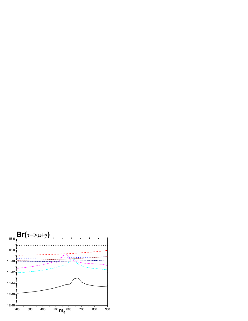
FIG. 1.: Illustrative plot for ${\rm BR}(\tau\rightarrow\mu+\gamma)$ changing with $m_{0}$. We take $\tan\beta=1.5$, $M_{L}=1\ {\rm Tev}$ and $M_{R}=20\ {\rm Tev}$ in our plot. Here the dot line corresponds to ${\cal F}_{1}$; the dash dot line corresponds to ${\cal F^{\prime}}_{1}$; the short dash line corresponds to ${\cal F}_{2}$; the short dash dot line corresponds to ${\cal F^{\prime}}_{2}$; the solid line corresponds to ${\cal F}_{3}$ and ${\cal F}_{4}$; the dash line corresponds to ${\cal F^{\prime}}_{3}$; the short dot line corresponds to ${\cal\cal F^{\prime}}_{4}$; the dot horizontal line corresponds to the experimental upper bound.

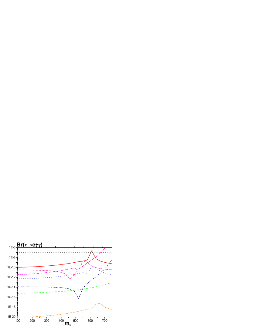
FIG. 2.: Illustrative plot for ${\rm BR}(\tau\rightarrow e+\gamma)$ changing with $m_{0}$. We take $\tan\beta=1.5$, $M_{L}=1\ {\rm Tev}$ and $M_{R}=20\ {\rm Tev}$ in our plot. Here the dash line corresponds to ${\cal F}_{1}$; the dot line corresponds to ${\cal F^{\prime}}_{1}$; the dash dot line correspond to ${\cal F}_{2}$; the dash dot dot line corresponds to ${\cal F^{\prime}}_{2}$; the solid line corresponds to ${\cal F^{\prime}}_{3}$; the short dash line corresponds to ${\cal F^{\prime}}_{4}$; the short dash line corresponds to ${\cal F}_{3}$ and ${\cal F}_{4}$; the dot horizontal line corresponds to the experimental upper bound.

REFERENCES

• [1] Super-Kamiokande Collaboration, Y. Fukuda et al., Phys. Rev. Lett. 81, 1562 (1998); Phys. Rev. Lett. 86, 5656 (2001).
• [2] SNO Collaboration, Q.R. Ahmad et al., Phys. Rev. Lett. 87, 071301 (2001); Phys. Rev. Lett. 89, 011302 (2002).
• [3] KamLAND Collaboration, K. Eguchi et al., Phys. Rev. Lett. 90, 021802 (2003).
• [4] CHOOZ Collaboration, M. Apollonio et al., Phys. Lett. B 420, 397 (1998); Palo Verde Collaboration, F. Boehm et al., Phys. Rev. Lett. 84, 3764 (2000).
• [5] K2K Collaboration, M.H. Ahn et al., Phys. Rev. Lett. 90, 041801 (2003).
• [6] A. Strumia and F. Vissani, hep-ph/0606054.
• [7] J.C. Pati and A. Salam, Phys. Rev. D 10, 275 (1974); R.N. Mohapatra and J.C. Pati, Phys. Rev. D 11, 566 (1975); Phys. Rev. D 11, 2558 (1975); G. Senjanovic and R.N. Mohapatra, Phys. Rev. D 12, 1502 (1975).
• [8] See, e.g., R.N. Mohapatra and P.B. Pal, Massive Neutrinos in Physics and Astrophysics, second edition (World Scientific, 1998).
• [9] R.M. Fracis, M. Frank and C.S. Kalman, Phys. Rev. D 43, 2369 (1990); R. Kuchimanchi and R.N. Mohapatra, Phys. Rev. D 48, 4352 (1993); Phys. Rev. Lett. 75, 3989 (1995); C. Ailakh, A. Melfo and G. Senjanovic, Nuovo Cim. A 110, 615 (1997); C. Aulakh, K. Benakli and G. Senjanovic, Phys. Rev. Lett. 79, 2188 (1997).
• [10] Z. Chacko and R.N. Mohapatra, Phys. Rev. D 58, 015001 (1998); C.S. Aulakh, A. Melfo, A. Rasin and G. Senjanovic, Phys. Rev. D 58, 115007 (1998); B. Dutta and R.N. Mohapatra, Phys. Rev. D 59, 015018 (1999); M. Frank, H. Konig and M. Pospelov, Eur. Phys. J. C 7, 135 (1999).
• [11] R.N. Mohapatra and G. Senjanovic, Phys. Rev. Lett. 44, 912 (1980); J. Schechterm and J.W.F. Valle, Phys. Rev. D 22, 2227 (1980); M. Magg and C. Wetterich, Phys. Lett. B 94, 61 (1980); G. Lazarides, Q. Shafi and C. Wetterich, Nucl. Phys. B 181, 287 (1981).
• [12] E.Kh. Akhmedov and M. Frogerio, Phys. Rev. Lett 96, 061802 (2006); E.Kh. Akhmedov and M. Frigerio, JHEP, 0701, 042 (2007); P. Hosteins, S. Lavignac and C.A. Savoy, Nucl. Phys. B 755, 137 (2006).
• [13] M. Frank, Phys. Rev. D 64, 053013 (2001).
• [14] J. Wess and B. Zumino, Phys. Lett. B 49, 52 (1979); J. Iliopoulos and B. Zumino, Nucl. Phys. B 76, 310 (1974).
• [15] W. Siegel, Phys. Lett. B 84, 193 (1979); D.M. Capper, D.R.T. Jones and P.V. Nieuwenhuizen, Nucl. Phys. B 167, 479 (1980); S. Antuch and M. Ratz, JHEP 0207, 059 (2002).
• [16] P.H. Chankowski and Z. Pluciennik, Phys. Lett. B 316, 312 (1993); K.S. Babu, C.N. Leung and J. Pantaleone, Phys. Lett. B 319, 191 (1993); S. Antusch, M. Drees, J. Kersten, M. Lindner and M. Ratz, Phys. Lett. B 519, 238 (2001); Phys. Lett. B 525, 130 (2002); S. Antusch, J. Kersten, M. Lindner, M. Ratz and M.A. Schmidt, JHEP 0503, 024 (2005); J.W. Mei, Phys. Rev. D 71, 073012 (2005); S. Luo, J.W. Mei and Z.Z. Xing, Phys. Rev. D 72, 053014 (2005); Z.Z. Xing, Phys. Lett. B 633, 550 (2006); Z.Z. Xing and H. Zhang, hep-ph/0601106; W. Chao and H. Zhang, Phys. Rev. D 75, 033003 (2007).
• [17] A. Brignole and A. Rossi, Nucl. Phys. B 701, 3 (2004); F.R. Joaquim and A. Rossi, Phys. Rev. Lett. 97, 181801 (2006); Nucl. Phys. B 765, 71 (2007).
• [18] Particle Data Group, W.M. Yao $et\ al$., J. Phys. G 33, 1 (2006).
• [19] N. Setzer and S. Spinner, Phys. Rev. D 71, 115010 (2005).
• [20] R. Barbieri, L.J. Hall and A. Strumia, Nucl. Phys. B 445, 219 (1995); J. Hisano, T. Moroi, K. Tobe and M. Yamaguchi, Phys. Rev. D 53 , 2442 (1996); J. Hisano and D. Nomura, Phys. Rev. D 59, 116005 (1999).
• [21] P.F. Harrison, D.H. Perkins, and W.G. Scott, Phys. Lett. B 530, 167 (2002); Z.Z. Xing, Phys. Lett. B 533, 85 (2002); P.F. Harrison and W.G. Scott, Phys. Lett. B 535, 163 (2002); X.G. He and A. Zee, Phys. Lett. B 560, 87 (2003).
• [22] A. Joshipura, E.A. Paschos and W. Rodejohann, Nucl. Phys. B 611, 227 (2001); JHEP 0108, 029 (2001); W. Chao, S. Luo and Z.Z. Xing, arXiv:0704.3838 [hep-ph].
• [23] MEGA Colloaboration, M.L. Brooks et al., Phys. Rev. Lett. 83, 1521 (1999); BARBAR Collaboration, B. Aubert et al., Phys. Rev. Lett. 96, 041801 (2006).
• [24] Super KEKB Physics Working Group, A.G. Akeroyd $et\ al$., hep-ex/0406071.
• [25] R.N. Mohapatra, Z. Phys. C 56, 117 (1992); M. Frank, Phys. Rev. D 65, 033011 (2002); K.S. Babu, B. Dutta and R.N. Mohapatra, Phys. Rev. D 67, 076006 (2003).
• [26] V. Lyubimov, E.G. Novikov, V.Z. Nozik, E.F. Tretyakov and V.S. Kosik, Phys. Lett. B 94, 266 (1980).
• [27] M. Frank, C.S. Kalaman and H.N. Saif, Z. Phys. C 59 655 (1993).
Refer to caption