Signal of Bose condensation in an optical lattice at finite temperature

Abstract

We discuss the experimental signal for the Bose condensation of cold atoms in an optical lattice at finite temperature. Instead of using the visibility of the interference pattern via the time-of-flight imaging, we show that the momentum space density profile in the first Brillouin zone, in particular its bimodal distribution, provides an unambiguous signal for the Bose condensation. We confirm this point with detailed calculations of the change in the atomic momentum distribution across the condensation phase transition, taking into account both the global trapping potential and the atomic interaction effects.

PACS numbers: 03.75.Lm, 03.75.Hh, 03.75.Gg

A recent work raised an interesting question on how to unambiguously confirm the Bose condensation associated with a superfluid phase at finite temperature for cold atoms in an optical lattice 1 ; 2 . The signal of Bose condensation in an optical lattice is typically connected with the interference peaks in the time-of-flight images. It is shown in 1 that for a thermal lattice gas above the condensation temperature, one could also see the interference peaks with a pretty good visibility 3 . This thermal visibility goes down considerably if one takes into account a number of practical effects, as shown in the recent work 4 . On the other hand, however, the thermal visibility above the transition temperature is not negligible, and its value depends on the details of a number of system parameters. There is no explicit critical value yet for the interference visibility to separate the condensation region from the thermal region.

In this work, we suggest to use the momentum space density profile in the first Brillouin zone (measured from the time-of-flight imaging) as an alternative method to characterize the Bose condensate in an optical lattice. In particular, similar to the free-space case, the bimodal distribution of the atomic momentum distribution should provide an unambiguous signal for the Bose condensation. To show the practicality of this method, we calculate the finite-temperature atomic momentum distribution in a three-dimensional (3D) optical lattice, confirming a distinctive change in the distribution across the condensation phase transition. There are several complexities in this calculation: first of all, one needs to take into account the inhomogeneity of the lattice due to the global harmonic trap, which tends to broaden the momentum distribution of the gas, in particular for the condensate part. Secondly, the atomic interaction leads to two competing effects: it broadens the real-space distribution and thus sharpens the momentum space density profile in a trap; while at the same time, it also leads to the broadening of the momentum distribution during the time-of-flight process. In our calculation, we take all these effects into account.

To illustrate the basic character of the experimental signal, first we calculate the finite temperature momentum distribution for free bosons in an optical lattice with a global harmonic trap, in which case exact solutions are possible after introducing some tricks. With the Feshbach resonance technique, one can also directly test the predictions in this case by turning off the atomic interaction. Then we use the Hatree-Fock-Bogliubov-Popov (HFBP) approximation 5 ; 6 ; 7 to deal with the interaction between the atoms. The HFBP method is expected to be a good approximation for weakly interacting bosons except for a small region across the transition from the superfluid phase to the normal phase 5 . For cold atoms in a lattice with a global harmonic trap, such a region corresponds to only a slim layer, which has negligible influence on the integrated momentum distribution. So we expect the HFBP approximation should be a reasonably good method for the calculation of the atomic momentum distribution before the Mott transition shows up in the trap. We note that the HFBP approximation has been used before for cold atoms, with the focus on the homogeneous case 6 or the one-dimensional system 7 .

For free bosonic atoms in an inhomogeneous optical lattice with a global harmonic trap, the Hamiltonian has the form $H=\int d\mathbf{r}\Psi^{{\dagger}}(\mathbf{r})[-(\hbar^{2}/2m)\partial_{\mathbf{r}}^{2}+V_{op}+V(\mathbf{r})]\Psi(\mathbf{r})$, where $m$ is the atomic mass, $V_{op}=V_{0}\sum_{i=1,2,3}\sin^{2}(\pi r_{i}/d)$ is the optical lattice potential with $d$ as the lattice spacing, and $V(\mathbf{r})=\frac{1}{2}m\omega^{2}\mathbf{r}^{2}$ is the global harmonic trapping potential. To diagonalize the Hamiltonian, we expand the atomic field operator $\Psi(\mathbf{r})$ as $\Psi(\mathbf{r})=\sum_{\mathbf{R}}w(\mathbf{r}-\mathbf{R})a_{\mathbf{R}}$, where the operator $a_{\mathbf{R}}$ ($a_{\mathbf{R}}$) annihilates (creates) a particle on site $R$, $w(\mathbf{r}-\mathbf{R})$ is the Wannier function on the site $\mathbf{R}$ associated with the lattice potential $V_{op}$, and the summation runs over all the lattice sites. A Fourier transform of this expansion gives

$$\Psi(\mathbf{k})=w(\mathbf{k})a_{\mathbf{k}},$$ (1)

where $\Psi(\mathbf{k}),w(\mathbf{k}),a_{\mathbf{k}}$ denote respectively the Fourier components of $\Psi(\mathbf{r}),w(\mathbf{r}),a_{\mathbf{R}}$ in the momentum space.

Under typical experimental situations, the global harmonic trap $V(\mathbf{r})$ varies slowly on individual lattice sites. In that case, under the expansion above, the Hamiltonian is recast into the form

$$H=\sum_{\mathbf{k}}E_{\mathbf{k}}a_{\mathbf{k}}^{{\dagger}}a_{\mathbf{k}}+\sum_{\mathbf{R}}V(\mathbf{R})a_{\mathbf{R}}^{{\dagger}}a_{\mathbf{R}},$$ (2)

where the summation over $\mathbf{k}$ runs over the first Brillouin zone. We have assumed here that the system temperature is well below the band gap, so the atoms only occupy the lowest band, where $E_{\mathbf{k}}$ is well approximated by $E_{\mathbf{k}}=-2t\sum_{i=1,2,3}\cos(k_{i}d)$. The parameter $t$ denotes the tunneling rate over the neighboring sites, with $t\approx\left(3.5/\sqrt{\pi}\right)V_{0}^{3/4}e^{-2\sqrt{V_{0}}}$ for an optical lattice 8 , where both $t$ and $V_{0}$ are in the unit of the recoil energy $E_{R}\equiv\hbar^{2}\mathbf{\pi}^{2}/2md^{2}$.

The Hamiltonian (2) in principle can be directly diagonalized numerically. However, the calculation of the finite temperature momentum distribution requires determination of all the eigenstates of the Hamiltonian, which is very time consuming for a three-dimensional lattice with many sites. Here, we adopt an approach which allows easy calculation of any finite temperature momentum distributions add1 ; add2 ; add3 . Note that the indices $\mathbf{R}$ and $\mathbf{k}$ in Eq. (2) are reminiscent of the coordinate and the momentum variables in quantum mechanics. So we can write down a first quantization Hamiltonian corresponding to Eq. (2) in the momentum space, where $\mathbf{R}$ is replaced by the momentum derivative $\partial_{\mathbf{k}}$. The resulting Hamiltonian takes the form

$$H_{eff}=-\frac{1}{2}m\omega^{2}\partial_{\mathbf{k}}^{2}+E_{\mathbf{k}}.$$ (3)

This Hamiltonian describes free particles with effective mass $m^{\ast}=\hbar^{2}/(m\omega^{2})$ trapped in an effective potential $E_{\mathbf{k}}$ with periodic boundary condition (the period is given by the reciprocal lattice vector $\mathbf{K}$). The quasi-momentum distribution $\left\langle a_{\mathbf{k}}^{{\dagger}}a_{\mathbf{k}}\right\rangle$ is then given by the square of the eigenstate wavefunctions $\left|\phi_{\mathbf{n}}\left(\mathbf{k}\right)\right|^{2}$ of $H_{eff}$, averaged over all the eigen-levels $\mathbf{n}$ with a Bose distribution factor $g(\epsilon_{\mathbf{n}})=1/\exp\left[\left(\epsilon_{\mathbf{n}}-\mu\right)/T-1\right]$ at finite temperature $T$, where $\epsilon_{\mathbf{n}}$ is the corresponding eigenenergy and $\mu$ is the chemical potential fixed by the total number of atoms. From Eq. (1), we then obtain the atomic momentum distribution

$$n(\mathbf{k}) = \left\langle\Psi^{\dagger}(\mathbf{k})\Psi(\mathbf{k})\right\rangle=\left|w(\mathbf{k})\right|^{2}\left\langle a_{\mathbf{k}}^{{\dagger}}a_{\mathbf{k}}\right\rangle$$ (4)

$$= \left|w(\mathbf{k})\right|^{2}\sum_{\mathbf{n}}g(\epsilon_{\mathbf{n}})\left|\phi_{\mathbf{n}}\left(\mathbf{k}\right)\right|^{2}$$

The signal from the time-of-flight imaging corresponds to the column integrated momentum distribution $n_{\perp}(k_{x},k_{y})=\int n(\mathbf{k})dk_{z}$.

Through Eq. (4), we have calculated the momentum distribution of a free Bose gas in an optical lattice with a global harmonic trap at different temperatures around the condensation transition. The parameters are chosen to be close to those of a typical experiment for ⁸⁷Rb, with the lattice barrier $V_{0}=10E_{R}$ and the total particle number $N\simeq 10^{5}$. The results for the integrated momentum distribution $n_{\perp}(k_{x},k_{y})$ are shown in Fig. 1 under different trap frequencies. In a weak harmonic trap, there are distinctive interference peaks even for a thermal gas above the transition temperature (Fig. 1(a)), which agrees with the result of Ref. 1 for a homogeneous optical lattice that corresponds to the zero-trap limit. These peaks are caused by the short range thermal correlations between different sites. The correlation function of the thermal gas decays exponentially with distance $x$ by the form $e^{-x/L}$, where the characteristic length $L$ is estimated to be $\sim 1.1d$ for Fig. 1(a). As the trap frequency increases, the thermal interference peaks become less visible and eventually disappear (Fig. 1(c)), which agrees with the recent calculation of the visibility in Ref. 4 . In the case of a weak global trap, it gets difficult to use the visibility to distinguish the condensation phase transition as this parameter has a pretty high value for both the condensed and the non-condensed phases near the critical temperature 1 ; 4 . However, if one directly compares the interference patterns in Figs. 1 (a,c) and (b,d) across the condensation transition, the difference in the interference peaks is still pretty clear: in particular, for the case with a condensate component, the interference peaks become much sharper. This reminds us to look at the momentum space density profile in the first Brillouin zone, which, compared with the single parameter of visibility, should be able to give more detailed information about the system and its phase transition.

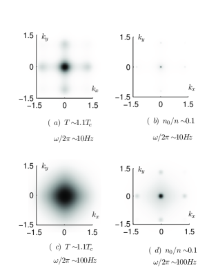
Figure 1: The intensity plot for the column integrated momentum distribution near the first Brillouin zone with different trapping frequency $\omega/2\pi$ and temperature $T$. Figs. (a) and (c) are for the normal phase, and (b) and (d) are for the superfluid phase with the corresponding parameters: (b) $T/T_{c}\sim 0.7$; (d) $T/T_{c}\sim 0.94$. The total particle number is fixed to be $N_{t}=10^{5}$ for all the cases, and the lattice barrier $V_{0}=10E_{R}$. The unit for the axes is $2\pi/d$.

With this in mind, we plot the column integrated momentum distribution along one of the axes passing through the center of the first Brillouin zone. The results are plotted in Fig. 2 (a) (c) (e) for different condensate fractions. It is clear that while the density profile is a thermal distribution for a normal gas, a bimodal structure appears when a non-zero condensate fraction exists in the lattice. Based on this observation, we propose to use the interference peaks as well as the bimodal structure in the first Brillouin zone as an unambiguous signature for detection of the Bose condensation in an optical lattice.

The calculation above is useful for an illustration of the general qualitative features of the system, but we neglect the interaction between the atoms in the lattice. In a more realistic model, such interactions need to be taken into account, as they can greatly modify the time-of-flight images. Firstly, the repulsive interaction will tend to broaden the spatial distribution of the atoms and hence narrow the momentum distribution in the trap. Secondly, in the process of the time-of-flight expansion, the remnant atomic interaction transforms the interaction energy into the kinetic energy, which shows up in the final imaging process and broadens the momentum distribution. In the presence of interaction, the system can not be solved exactly. In the following, we calculate the momentum distribution of an interacting Bose gas in an optical lattice with a global harmonic potential trap using the Hatree-Fock-Bogliubov-Popov (HFBP) approximation 5 .

To calculate the momentum space density profile for an atomic gas in an inhomogeneous optical lattice, we combine the HFBP method with the local density approximation (LDA). Under the LDA, a local region of the harmonic trap is treated as a homogeneous lattice system. We first look at the Hamiltonian with inter-atomic interaction for a homogeneous lattice gas:

$$H=-t\sum_{\langle\mathbf{i,j}\rangle}a_{\mathbf{i}}^{{\dagger}}a_{\mathbf{j}}+\frac{U}{2}\sum_{\mathbf{i}}a_{\mathbf{i}}^{{\dagger}}a_{\mathbf{i}}^{{\dagger}}a_{\mathbf{i}}a_{\mathbf{i}}-\mu\sum_{\mathbf{i}}a_{\mathbf{i}}^{{\dagger}}a_{\mathbf{i}}$$ (5)

where $t$ is the tunneling rate defined before, $\mu$ is the local chemical potential, $U=U_{bg}\int|w(\mathbf{r})|^{4}d\mathbf{r}$ is the on-site interaction rate with an approximate form of $U/E_{R}\approx 3.05(V_{0}/E_{R})^{0.85}(a_{s}/d)$ ($U_{bg}$ is related to the s-wave scattering length by $U_{bg}=4\pi\hbar^{2}a_{s}/m$, and $a_{s}=5.45nm$ for ⁸⁷Rb 1 ; 3 ). We then transform all the field operators to the momentum space, and write the momentum component $a_{\mathbf{k}}$ as $a_{\mathbf{k}}=v\delta_{\mathbf{k0}}+\delta a_{\mathbf{k}}$ with the standard HFBP approach, where $v\equiv\langle a_{\mathbf{0}}^{{\dagger}}\rangle\equiv\left\langle a_{\mathbf{0}}\right\rangle$ represents the condensate fraction, and $\delta a_{\mathbf{k}}$ and $\delta a_{\mathbf{k}}^{{\dagger}}$ represent the excitations above the mean field. We keep the Hamiltonian to the quadratic order of the operators $\delta a_{\mathbf{k}}$ and $\delta a_{\mathbf{k}}^{\dagger}$, and then diagonalize it to get the thermal potential $\Omega=-T\ln tr\left(e^{-H/T}\right)$. The stationary condition $\partial\Omega/\partial v=0$ gives the saddle point equation for the chemical potential:

$$\mu=E_{0}-Un_{0}+2Un,$$ (6)

where $E_{0}=-6t$ for a three-dimensional system, $n_{0}$ is the per-site density of the condensate fraction, and $n$ is the total number of particles per site. With the thermal potential, it is easy to derive the number equation and the atomic momentum distribution. For the non-condensate part with $\mathbf{k}\neq 0$, the per-site quasi-momentum density distribution $\left\langle a_{\mathbf{k}}^{{\dagger}}a_{\mathbf{k}}\right\rangle$ is given by

$$\left\langle a_{\mathbf{k}}^{{\dagger}}a_{\mathbf{k}}\right\rangle=\frac{E_{\mathbf{k}}-E_{0}+Un_{0}}{2\hbar\omega_{\mathbf{k}}}\coth\left(\frac{\hbar\omega_{\mathbf{k}}}{2T}\right)-\frac{1}{2},$$ (7)

where $\hbar\omega_{\mathbf{k}}=\sqrt{(E_{\mathbf{k}}-E_{0})^{2}+2Un_{0}(E_{\mathbf{k}}-E_{0})}$ is the dispersion relation for the Bogliubov excitations. With the LDA, the local chemical potential $\mu(\mathbf{r})$ at a displacement $\mathbf{r}$ from the trap center is determined from $\mu(\mathbf{r})=\mu_{0}-V(\mathbf{r})$, where $\mu_{0}$ is the chemical potential at the trap center. We fix the total number density per-site at the trap center, which, together with Eqs. (6-7) and the number equation $n=n_{0}+\sum_{\mathbf{k}\neq 0}\left\langle a_{\mathbf{k}}^{{\dagger}}a_{\mathbf{k}}\right\rangle$, allow us to calculate the chemical potential $\mu_{0}$. We may then determine $\mu(\mathbf{r})$ and $\left\langle a_{\mathbf{k}}^{{\dagger}}a_{\mathbf{k}}\right\rangle$ at any trap location $\mathbf{r}$. The overall non-condensate part of the atomic momentum distribution is given by the integration of $\left\langle a_{\mathbf{k}}^{{\dagger}}a_{\mathbf{k}}\right\rangle$ over the whole harmonic trap, multiplied by the Wannier function $\left|w(\mathbf{k})\right|^{2}$ as shown in Eq. (4).

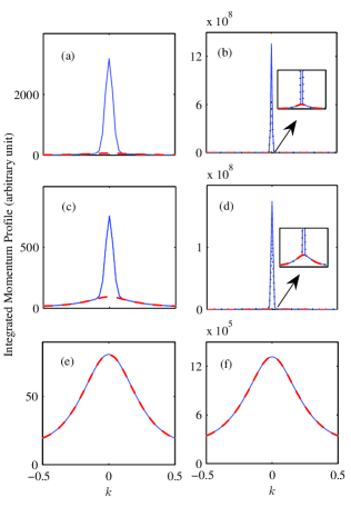
Figure 2: (Color online) Column integrated momentum density profile (shown along the x-axis) for (a)(c)(e) non-interacting lattice bosons and (b)(d)(f) interacting lattice bosons. The solid curves are the total momentum density profile; the thick dashed curves are the momentum density profile of the normal component; the dotted curves are the momentum density profile taking into account of the interaction broadening during the time-of-flight evolution. (a) $N_{0}/N_{t}\sim 0.46$, $T/T_{c}\sim 0.75$ ($N_{0}$ is the total number of atoms in the condensate and $N_{t}$ is the total number of atoms in the trap); (b) $N_{0}/N_{t}\sim 0.52$, $T/T_{c}\sim 0.34$; (c) $N_{0}/N_{t}\sim 0.10$, $T/T_{c}\sim 0.95$; (d) $N_{0}/N_{t}\sim 0.10$, $T/T_{c}\sim 0.65$, inset: enlarged density profile below the dotted line; (e) $T\sim 1.1T_{c}$; (f) $T\sim 1.1T_{c}$. For the non-interacting calculations, the total particle number is fixed to be $N_{t}=10^{5}$, and the trapping frequency is $\omega/2\pi=20Hz$; for the calculations with interactions, the trapping potential is $\omega/2\pi=20Hz$, the number density per-site at the center of the trap is fixed to be $n(0)=1$, with the total number of particles on the order of $N_{t}=10^{5}\sim 10^{6}$. The lattice barrier in all the cases is $V_{0}=10E_{R}$. The unit for the x-axes is $2\pi/d$.

For the condensate part, the LDA will lead to an artificial $\delta$-function at zero momentum. To avoid this artifact, one needs to consider explicitly the broadening of the condensate momentum distribution by the harmonic trap. From the above LDA formalism, we get the condensate fraction $n_{0}(\mathbf{r})$ at any trap location $\mathbf{r}$. The condensate wavefunction in the trap can be well approximated by $\phi_{0}(\mathbf{r})=\sqrt{n_{0}(\mathbf{r})}$ (which actually corresponds to the solution of the Gross-Pitaevskii equation under the Thomas-Fermi approximation 9 ). The condensate part of the atomic momentum distribution is thus given by the Fourier-transform of the wave function $\phi_{0}(\mathbf{r})$. The resulting momentum distribution is then added to the momentum profile of the normal gas which is typically at the edge of the trap. We plot the results of our calculation in Fig. 2 (b)(d)(f). In general, the peaks are now sharper compared to the case of an ideal Bose gas, which is just as expected. A bimodal distribution still shows up when the condensate fraction becomes non-zero (Fig. 2(d)). In real experiments, due to the finite resolution in imaging, the height of the central condnesate peak will be significantly reduced, and the bimodal structure will become more pronounced and should be readily observable.

After turnoff of the trap, the atomic momentum distribution will be broadened during the time-of-flight process due to the collision interaction. The interaction broadening of the momentum distribution happens dominantly through the condensate fraction 2 ; 4 , for which one has a higher number density and a smaller expansion speed. To incorporate this effect, we use the Gross-Pitaevskii equation 9 to solve the evolution of the condensate wavefunction $\phi_{0}(\mathbf{r,}t)$, starting at $\phi_{0}(\mathbf{r})$ when the expansion time $t=0$. The Fourier component of $\phi_{0}(\mathbf{r,}t)$ after a long enough expansion gives the final momentum distribution for the condensate part. The results of the calculation are shown in Fig.2 (b) (d) for ⁸⁷Rb atoms. One can see that the interaction broadening leads to some quantitative corrections of the profile by lowering its peak value, but it does not change much the overall picture. In particular, the bimodal structure remains similar when there is a condensate fraction.

In summary, we have shown through explicit calculation that the interference peaks, combined with the bimodal profile of the central peak in the first Brillouin zone, provide an unambiguous signal for the condensation phase transition for cold atoms in an optical lattice at finite temperature. We develop some techniques to calculate the atomic density profile, in particular for an inhomogeneous system with a global harmonic trap. In general, the density profile of the interference peak gives more detailed information of the system, and a comparison of the density profiles from the theoretical calculation and from the experimental observation will contribute to the understanding of this strongly correlated system at finite temperature.

This work was supported by the NSF awards (0431476), the ARDA under ARO contracts, and the A. P. Sloan Fellowship.

References

- (1) R. B. Diener, Q. Zhou, H. Zhai, and T.-L. Ho, Phys. Rev. Lett. 98, 180404 (2007).
- (2) For a review on optical lattice, see I. Bloch and M. Greiner, Adv. At. Mol. Phys. 52, 1-47 (2005).
- (3) F. Gerbier et al., Phys. Rev. A 72, 053606 (2005).
- (4) F. Gerbier, S. Foelling, A. Widera, and I. Bloch, cond-mat/0701420.
- (5) J. O. Andersen, Rev. Mod. Phys. 76, 599 (2004).
- (6) D. van Oosten, P. van der Straten, and H. T. C. Stoof, Phys. Rev. A 63, 053601 (2001).
- (7) A. M. Rey et al., cond-mat/0210550.
- (8) L.-M. Duan, Phys. Rev. Lett. 95, 243202 (2005).
- (9) A. Polkovnikov, S. Sachdev, and S. M. Girvin, Phys. Rev. A 66, 053607 (2002).
- (10) C. Hooley and J. Quintanilla, Phys. Rev. Lett. 93, 080404 (2004).
- (11) A. M. Rey, G. Pupillo, C. W. Clark, and C. J. Williams, Phys. Rev. A 72, 033616 (2005).
- (12) F. Dalfovo, S. Giorgini, L. P. Pitaevskii, and S. Stringari, Rev. Mod. Phys. 71, 463 (1999).