Numerical Study on Stellar Core Collapse and Neutrino Emission:
Probe into the Spherically Symmetric Black Hole Progenitors with 3 - 30$M_{\odot}$ Iron Cores

Abstract

The existence of various anomalous stars, such as the first stars in the universe or stars produced by stellar mergers, has been recently proposed. Some of these stars will result in black hole formation. In this study, we investigate iron core collapse and black hole formation systematically for the iron-core mass range of 3 - 30$M_{\odot}$, which has not been studied well so far. Models used here are mostly isentropic iron cores that may be produced in merged stars in the present universe but we also employ a model that is meant for a Population III star and is obtained by evolutionary calculation. We solve numerically the general relativistic hydrodynamics and neutrino transfer equations simultaneously, treating neutrino reactions in detail under spherical symmetry. As a result, we find that massive iron cores with $\sim 10M_{\odot}$ unexpectedly produce a bounce owing to the thermal pressure of nucleons before black hole formation. The features of neutrino signals emitted from such massive iron cores differ in time evolution and spectrum from those of ordinary supernovae. Firstly, the neutronization burst is less remarkable or disappears completely for more massive models because the density is lower at the bounce. Secondly, the spectra of neutrinos, except the electron type, are softer owing to the electron-positron pair creation before the bounce. We also study the effects of the initial density profile, finding that the larger the initial density gradient is, the more steeply the neutronization burst declines. Further more, we suggest a way to probe into the black hole progenitors from the neutrino emission and estimate the event number for the currently operating neutrino detectors.

1 Introduction

Various anomalous stars, such as the first stars in the universe (so-called Population III stars) or stars produced by stellar mergers in stellar clusters, are being studied recently. As for the Population III stars, it is suggested theoretically that they are much more massive ($M\gtrsim 100M_{\odot}$) than stars of later generations (e.g., Nakamura & Umemura 2001). On the other hand, $N$-body simulations show that the runaway mergers of massive stars occur and that very massive ($M\gtrsim 100M_{\odot}$) stars are formed in a young compact stellar cluster (e.g., Portegies Zwart 1999). Especially notable is a newly suggested formation scenario for supermassive black holes which requires the formation of intermediate-mass black holes by the collapse of merged stars in very compact stellar clusters (e.g., Ebisuzaki et al. 2001). If these anomalous stars collapse to black holes without supernova explosions, it is supposedly difficult to be hard to probe into their progenitors. One possible means of such a probe is, we think, to examine the neutrinos emitted during the black hole formation. For this purpose, systematic studies on black hole formation, including effects of the neutrinos, are needed.

So far, various numerical simulations of supernova explosions have been done by many authors. Similarly, numerical studies on black hole formation have also been recently produced (e.g., Fryer 1999; Linke et al. 2001; Fryer et al. 2001, hereafter FWH01; Sekiguchi & Shibata 2005, hereafter SS05; Nakazato et al. 2006, hereafter NSY06; Sumiyoshi et al. 2006, hereafter SYSC06). Fryer (1999) classified core collapse into three types. a) Stars with $M\lesssim 25M_{\odot}$ make explosions and produce neutron stars. b) Stars ranging $25M_{\odot}\lesssim~{}M\lesssim 40M_{\odot}$ also result in explosions but produce black holes via fallback. c) For $M\gtrsim 40M_{\odot}$, the shock produced at the bounce can neither propagate out of the core nor make explosions. In any case, the core bounces once. SYSC06 computed fully general relativistic hydrodynamics under spherical symmetry, taking into account the reactions and transports of neutrinos in detail and confirmed class c) for the collapse of a progenitor with $40M_{\odot}$. On the other hand, much more massive stars result in black hole formation without bounce. SS05 studied the criterion for the collapse without bounce. Their computations are fully general relativistic, and they investigated the dynamics systematically, varying the initial mass and rotation. They concluded that non-rotating iron cores with a mass of $M_{\mathrm{iron}}\gtrsim 2.2M_{\odot}$ collapse to black holes without bounce. However, they employed the phenomenological equation of state and did not consider the effects of neutrinos.

There are studies also on a collapse of very massive stars in a context of the evolution of Population III stars. As mentioned already, Population III stars may be very massive, $M\gtrsim 100M_{\odot}$. It is supposed that the pair creation of electrons and positrons makes a star unstable during the helium burning phase if they do not lose much of their mass during the quasi-static evolutions because of zero metallicity. Stars with $\lesssim 260M_{\odot}$ reverse the collapse by rapid nuclear burnings and explode to pieces, which are called pair-instability supernovae, while more massive stars cannot halt the collapse and form black holes (e.g., Heger et al. 2003). Note that, however, these numbers are still uncertain at present (e.g., Ohkubo et al. 2006). Assuming that Population III stars with $M\gtrsim 300M_{\odot}$ are formed and evolve without mass loss, FWH01 and NSY06 showed that they collapse without bounce for spherically symmetric models under fully general relativistic computations while NSY06 treated the neutrino transport more in detail than FWH01. FWH01 also computed the collapse of a rotating star with $300M_{\odot}$ under Newtonian gravity and showed that it has a weak bounce and then recollapses to a black hole immediately. As for the collapse of supermassive stars with $M\gtrsim 5\times 10^{5}M_{\odot}$, Linke et al. (2001) found that they form black holes without bounce before becoming opaque to neutrinos.

The black hole formation of stars in the mass range between $\sim 100M_{\odot}$ and $\sim 260M_{\odot}$, which corresponds to the iron-core mass range between $\sim 3M_{\odot}$ and $\sim 30M_{\odot}$, has not been studied well so far. This is because they are supposed to explode as pair-instability supernovae during the quasi-static evolutions if they are single stars. Recently, on the other hand, stars produced by stellar mergers in a young compact stellar cluster were studied in detail and their evolutionary paths are beginning to be revealed (Suzuki et al. 2007). While they do not calculate the evolutions of these stars up to the black hole formation, we speculate, as in § 3.5.1, that they may avoid the explosions as pair-instability supernovae and form a massive iron core of the above-mentioned range. Therefore, we investigate, in this study, the iron core collapses systematically for the iron core masses of $3M_{\odot}$ and $30M_{\odot}$, although there is no evidence to show their existence so far.

To be more specific, we assume that the mass of an iron core is mainly determined by the entropy per baryon, and our investigation is done systematically for entropy. We solve the general relativistic hydrodynamics under spherical symmetry. We also solve the neutrino transfer equations simultaneously, treating neutrino reactions in detail. In addition to the isentropic iron core models, we employ the realistic stellar model of $100M_{\odot}$ and zero metallicity, supposedly a Population III star, by Nomoto et al. (2005). We address the issues concerning the black hole formation of the merged stars in connection with our study and estimate the neutrino event number for the currently operating detectors. We also suggest a way to probe into the progenitors from the detection. We hope that this study will be not only a reference for future multi-dimensional computations but also provide a basis for neutrino astrophysics in the black hole formation.

2 Initial Models and Numerical Methods

At first, we construct the iron core models, which will later be used as initial models for the dynamical simulation of the collapse. The progenitor with $40M_{\odot}$ in SYSC06 has an entropy per baryon, $s\sim 1.5k_{B}$ and an iron core mass, $M_{\mathrm{iron}}=1.98M_{\odot}$, whereas the massive Population III star models in NSY06 have $s>16k_{B}$ and $M_{\mathrm{iron}}>50M_{\odot}$. In this study, we intend to bridge the gap of the black hole progenitors and discuss the neutrino emission systematically for this range. Unfortunately, realistic models of the progenitors for this range are rare, and “systematic” models for them are absent up to the present, since their astrophysical counterparts are not well known, as mentioned already. Therefore, we construct the initial models by ourselves.

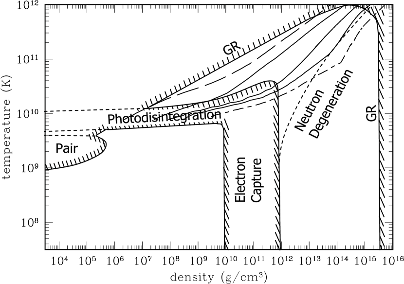
Figure 1: The evolution of the central density and temperature for various models which result in black hole formation. The dot-dashed line is for a realistic progenitor with the initial mass $40M_{\odot}$ in SYSC06 and the long-dashed line is for a Population III star with the initial mass $10500M_{\odot}$ ($s=74.75k_{\mathrm{B}}$) in NSY06. Three solid lines are for our models in this paper, and each line corresponds to model 1a ($s=3k_{\mathrm{B}}$), 3a ($s=5k_{\mathrm{B}}$) and 5a ($s=10k_{\mathrm{B}}$), from right to left. The shaded area represents a gravitationally unstable region by labeled physical processes.

We assume that the iron cores in equilibrium configurations collapse by photodisintegration, as is the case for the onset of ordinary core collapse supernovae. We obtain the initial models, solving the Oppenheimer-Volkoff equation with the equation of state by Shen et al. (1998a, 1998b) assuming isentropy and the electron fraction $Y_{e}=0.5$ throughout the core. We define the mass of the iron core, $M_{\mathrm{iron}}$, as the mass coordinate where the temperature is $5\times 10^{9}$ K, whereas we set the outer boundary at a much larger radius so as not to affect the dynamics. For the systematic analysis, we set the initial central temperature as $T_{\mathrm{initial}}=7.75\times 10^{9}$ K, which is slightly higher than the critical temperature for the photodisintegration (Figure 1), and generate models 1a-6a with the values of entropy per baryon, $s=3k_{B}$-$13k_{B}$, which have not been studied well so far, as mentioned above. In order to investigate the ambiguity in the onset of collapse, we also adopt a model (model 2b) with the same initial entropy per baryon as model 2a ($s=4k_{B}$) but having half the central density. The key parameters of these models are summarized in Table 1. In addition, we also employ the realistic stellar model of $100M_{\odot}$ with a vanishing metallicity by Nomoto et al. (2005) in order to validate the isentropic models. This model is supposedly a Population III star and resides in the range $s=3k_{B}$-$13k_{B}$.

As a next step, we compute the dynamics of spherically symmetric gravitational collapse with the neutrino transport. As for our numerical methods, we follow NSY06 and use the general relativistic implicit Lagrangian hydrodynamics code, which solves simultaneously the neutrino Boltzmann equations (Yamada 1997 ; Yamada et al. 1999 ; Sumiyoshi et al. 2005). We consider four species of neutrino, $\nu_{e}$, $\bar{\nu}_{e}$, $\nu_{\mu}$ and $\bar{\nu}_{\mu}$, assuming that $\nu_{\tau}$ and $\bar{\nu}_{\tau}$ are the same as $\nu_{\mu}$ and $\bar{\nu}_{\mu}$, respectively, and take into account 9 neutrino reactions listed in NSY06. We use 127 radial mesh points, while 12 and 4 mesh points are used for energy- and angular distribution of neutrino, respectively. In order to assess the convergence of our results, we compute models with higher resolutions. They have the same initial conditions as model 2a. For model 2m, the number of radial mesh points is increased to 255. Model 2e use 18 mesh points for the energy spectrum while model 2g has 6 mesh points for the angular distribution.

It is noted that our method allows us to follow the dynamics with no difficulty up to the apparent horizon formation. The existence of the apparent horizon is the sufficient condition for the formation of a black hole (or, equivalently, of an event horizon). For the Misner-Sharp metric (Misner & Sharp 1964) adopted in our computations, the radius of the apparent horizon is written as

$$r=\frac{2G\widetilde{m}}{c^{2}},$$ (1)

where $c$ and $G$ are the velocity of light and the gravitational constant, respectively (van Riper 1979). $r$ is the circumference radius and $\widetilde{m}$ is the gravitational mass inside $r$. Since our models are spherically symmetric, there is no difficulty in finding the horizon.

3 Results and Discussions

In this section, we show the results of our computations and discuss them. We study the dynamics of the collapse in § 3.1 and investigate the features of the neutrinos emitted during the collapse in § 3.2. In § 3.3, we investigate the role of the initial velocity or the deviation from equilibrium. We also make a comparison with the realistic progenitor models in § 3.4. Finally, we mention about the astronomical counterparts of our models and the possibility of the probe into the progenitors of the events in § 3.5.

To overview the characteristics of the models which we surveyed, we show in Figure 1, the evolution of the central density and temperature of our results together with those of other simulations of black hole formation. The trajectories of the current models shown by solid lines are between those of previous models reflecting the different values of entropy. From this figure, we can recognize that our investigation bridges the gap between two previous studies, SYSC06 and NSY06.

3.1 Dynamical Features

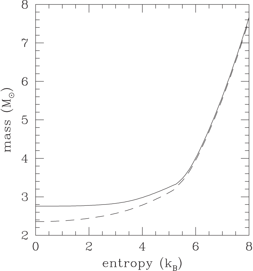
Figure 4: The maximum mass of the neutron star assuming isentropy and a constant electron fraction which is isentropic ($Y_{e}=0.1$) under the equation of state by Shen et al. (1998a, 1998b). The solid and dashed lines represent the maximum mass in the sense of the baryon rest mass and the gravitational mass, respectively.

It is known that ordinary supernovae with $s\sim 1k_{\mathrm{B}}$ bounce because their central density exceeds the nuclear density ($\sim 2.5\times 10^{14}\mathrm{g\,cm^{-3}}$) and pressure drastically increases. From our computations, we find that models with $3k_{\mathrm{B}}\leq s\leq 7.5k_{\mathrm{B}}$ ($M\leq 10.6M_{\odot}$) have a bounce and that they recollapse to black holes. On the other hand, models with $s>7.5k_{\mathrm{B}}$ ($M>10.6M_{\odot}$) collapse to black holes directly without bounce. We show the evolution of core collapse in Figure 4 for two representative cases.

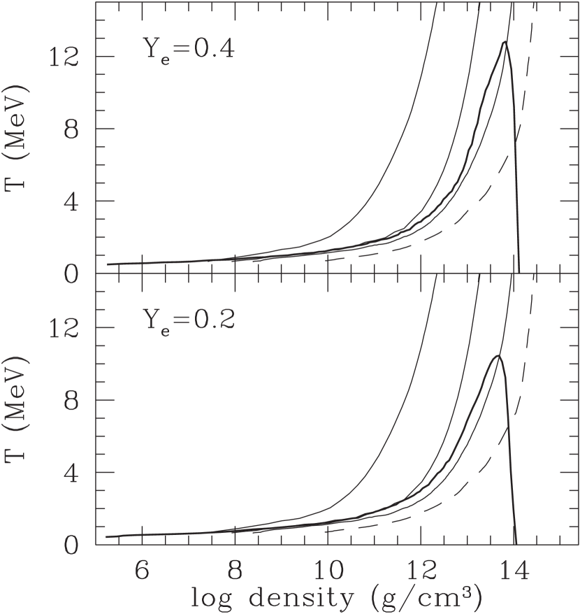
Figure 3: Phase diagram in $\rho-T$ plane from Shen et al. (1998b) for fixed electron fraction, $Y_{e}$ (thick lines). The nucleus exists in the region below these thick lines. The phase boundaries depend on $Y_{e}$, whereas the same trajectories are plotted for the upper panel and the lower panel. The dashed line represents the evolution of the central density and temperature for the ordinary supernova progenitor with the initial mass $15M_{\odot}$ (Sumiyoshi et al. 2005), and the solid lines do the same for the progenitors studied. Each line corresponds to models 1a ($s=3k_{\mathrm{B}}$), 3a ($s=5k_{\mathrm{B}}$) and 5a ($s=10k_{\mathrm{B}}$), from right to left.

In the case of $3k_{\mathrm{B}}\leq s\leq 7.5k_{\mathrm{B}}$, it is noted that the bounce mechanism of the core with $s\geq 3k_{\mathrm{B}}$ is not the same as that of ordinary supernovae. The high entropy cores bounce because of the thermal pressure of nucleons at sub-nuclear density. We can see this fact from the evolutions of central density and temperature in the phase diagram of the nuclear matter at $Y_{e}=0.4$ and $0.2$ (Figure 3). We note that for all models at the center, $Y_{e}\sim 0.4$ and $Y_{e}\sim 0.2$ when $T\sim 1$ MeV and $T\sim 10$ MeV, respectively. These figures show that the models with higher entropies go from the non-uniform mixed phase of nuclei and free nucleons to the classical ideal gas phase of thermal nucleons and $\alpha$ particles, whereas that of an ordinary supernova goes into the uniform nuclear matter phase. In the ideal gas phase, the number of non-relativistic nucleons and $\alpha$ particles is comparable to that of relativistic electrons. Since the adiabatic index of non-relativistic gas is $\gamma=\frac{5}{3}$ and that of relativistic gas is $\gamma=\frac{4}{3}$, the collapse is halted and bounce occurs.

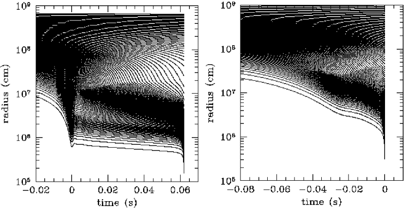
Figure 2: Radial trajectories of mass elements. The left panel is for model 2a ($s=4k_{B}$); time is measured from the bounce. The right panel is for model 5a ($s=10k_{B}$); time is measured from the point at which the apparent horizon is formed.

Because this bounce is weak and the shock is stalled, the inner core (or the protoneutron star) grows beyond the maximum mass of the neutron star and recollapses to a black hole soon (left panel of Figure 2). In Figure 4, we show the maximum mass of the neutron star assuming isentropy and the constant electron fraction ($Y_{e}=0.1$) under the equation of state by Shen et al. (1998a, 1998b). It is noted that the maximum mass is larger than $3M_{\odot}$ for the neutron star with high entropies, $s\gtrsim 4k_{\mathrm{B}}$. Since the maximum mass of the neutron star depends on the equation of state, it should be remind that the time interval from the bounce to the recollapse also depends on it (SYSC06). We will refer to this point again later.

In Table 1, we show the inner core mass, central density, temperature and adiabatic index at the bounce together with the interval time from the bounce to the apparent horizon formation. We can recognize that the density and the adiabatic index at the bounce get lower for the models with higher initial entropies. These features indicate that the bounce is not due to the nuclear force but to the thermal pressure of non-relativistic gas for high entropy cores. Moreover, the interval time from the bounce to the apparent horizon formation is shorter for the higher entropy cores. This is because the initial mass of the iron core ($M_{\mathrm{iron}}$) is larger than the maximum mass of the neutron star ($M_{\mathrm{max}}$) for the models with high entropies and they can collapse to black holes quickly.

We also show the results for the models with higher resolutions in Table 1. The central density and the adiabatic index at bounce, which are key parameters in our analysis, are not very different for models 2a, 2g and 2m. The central density at bounce of model 2e, which has 1.5 times finer energy mesh, is different by 14% from that of model 2a. This is because neutrinos affect the entropy variations before the neutrino trapping. In fact, the central entropy at bounce of model 2a is $3.50k_{\mathrm{B}}$ while that of model 2e is $3.62k_{\mathrm{B}}$. However, qualitative features of their bounces are not changed. On the other hand, the interval times from the bounce to the apparent horizon formation are different by $\lesssim$ 15% for models 2a, 2e, 2g and 2m. This is because the start point of the recollpase is roughly determined by the maximum mass of the neutron star as mentioned already. Since the mass accretion rate is of the order of $10M_{\odot}\,\mathrm{s}^{-1}$ during this phase in our models, the difference of $0.1M_{\odot}$ in the maximum mass means the difference of 10ms in the interval time, which is close to the discrepancies found here. Thus, the precise determination of the interval time is difficult in general. However, its dependence on the initial entropy is well established.

We compare our results with other studies. In SS05, the non-rotating models with an iron core mass of $\gtrsim 2.28M_{\odot}$ end up with black holes without bounce. In our models, on the other hand, it is shown that the iron core with $\lesssim 10.6M_{\odot}$ (or the initial entropy $s\lesssim 7.5k_{\mathrm{B}}$) has bounce before black hole formation. This discrepancy comes from the fact that their equation of state is parametric and does not take into account properly the effects of thermal nucleons in the collapsing phase. On the other hand, the rotating Population III star with $\sim 300M_{\odot}$ has a weak bounce at $\rho_{c}\sim 10^{12}\mathrm{g\,cm^{-3}}$ in FWH01, and these authors adopt a realistic equation of state (Herant et al. 1994). Since the rotation tends to produce a bounce, we can predict that the bounce is inevitable for an iron core with the mass $\lesssim 10M_{\odot}$ irrespective of rotations, and the effects of thermal nucleons are crucial.

In the high entropy case $s>7.5k_{\mathrm{B}}$, more massive cores do not have a bounce but form an accretion shock before the apparent horizon formation. This is because, the outer region keeps collapsing supersonically while the central region becomes gravitationally stable by the thermal pressure of non-relativistic gas. We can see this feature in the right panel of Figure 2. As the initial mass gets larger, the transition occurs smoothly from the collapse with bounce to the one without bounce. Incidentally, the features of direct collapse are almost the same as those for the Population III models in NSY06, where a detailed analysis can be found.

3.2 Neutrino Signals

In this section, we discuss neutrino emission during core collapse. As mentioned already, we compute the collapse until the formation of the apparent horizon. However, the location of the event horizon is not known for our models although it is proved mathematically that the event horizon is always located outside the apparent horizon. Moreover, the numerical difficulty prevents us from computing the dynamics until the apparent horizon swallows the shock surface entirely. Because of these facts, the total energy and number of emitted neutrinos have some ambiguities. In this study, we estimate the upper and lower limits for the total energy and number of emitted neutrinos, following NSY06. The upper limit is obtained with an assumption that all neutrinos in the region between the shock surface and the neutrino sphere flow out without being absorbed or scattered. For the lower limit, on the other hand, we assume that all neutrinos in this region are trapped and do not come out. Fortunately, for the models with bounce, these ambiguities are minor, compared with the direct collapse models in NSY06, since the duration from the shock formation to the apparent horizon formation is longer and almost all neutrinos are emitted during this phase.

The calculated results of the neutrino emission are summarized in Table 2. It is noted that we assume that $\nu_{\tau}$ ($\bar{\nu}_{\tau}$) is the same as $\nu_{\mu}$ ($\bar{\nu}_{\mu}$), and that the luminosities of $\nu_{\mu}$ and $\bar{\nu}_{\mu}$ are almost identical because they have the same reactions and because the difference of coupling constants is minor. In the following, ignoring this tiny difference, we denote these four species as $\nu_{x}$ collectively. In Table 2, we can recognize that the total energy does not change monotonically with the initial entropy of the core. This is because the duration of the neutrino emission is longer for the lower entropy models, while the duration is shorter and the neutrino luminosity is larger for the higher entropy models.

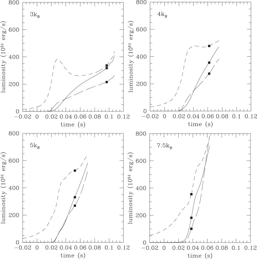
Figure 5: Luminosities of $\nu_{e}$ (short-dashed line), $\bar{\nu}_{e}$ (solid line) and $\nu_{x}$ (long-dashed line) as a function of $t$, where $\nu_{x}$ stands for $\mu$- and $\tau$-neutrinos and their anti-particles. Squares show the time when the apparent horizon is formed. Upper left, upper right, lower left and lower right panels are for models 1a ($s=3k_{\mathrm{B}}$), 2a ($s=4k_{\mathrm{B}}$), 3a ($s=5k_{\mathrm{B}}$) and 4a ($s=7.5k_{\mathrm{B}}$), respectively.

In Figure 5, we show the time evolutions of neutrino luminosity for several models under the assumption that the neutrinos outside the neutrino sphere flow freely after the apparent horizon formation. As already mentioned, the time interval from the bounce to the apparent horizon formation depends on the equation of state. In SYSC06, it is shown that the features of the neutrino emission, such as a neutronization burst, are not sensitive to the equation of state very much for the early phase. From Figure 5, we can see that the sign of neutronization burst becomes less remarkable and disappears for the higher entropy models.

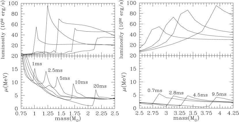
Figure 6: Snapshots of the profiles for the luminosity and the chemical potential of an electron-type neutrino. The left panel corresponds to the model 1a ($s=3k_{\mathrm{B}}$) and the right to the model 4a ($s=7.5k_{\mathrm{B}}$).

In order to analyze these features, we discuss the neutrino emission from model 1a, as a reference model. In the upper left panel of Figure 6, we show snapshots of the luminosity of an electron-type neutrino as a function of the baryon mass coordinate. We can recognize that neutrinos are emitted on the shock surface mainly. The luminosity on the shock surface has a peak (e.g., at $1.25M_{\odot}$ in the upper left panel of Figure 6), which is similar to the situation for ordinary supernovae (e.g., Thompson et al. 2003). In the following, we estimate the value of the luminosity semi-analytically and compare it with the results of our numerical simulations.

At first, the number density of neutrinos on the shock surface can be evaluated roughly by the equilibrium value,

$$n_{\mathrm{eq.}}(\epsilon)d\epsilon\propto\frac{\epsilon^{2}}{\exp\left(\frac{\epsilon-\mu_{\nu}}{k_{\mathrm{B}}T}\right)+1}d\epsilon,$$ (2)

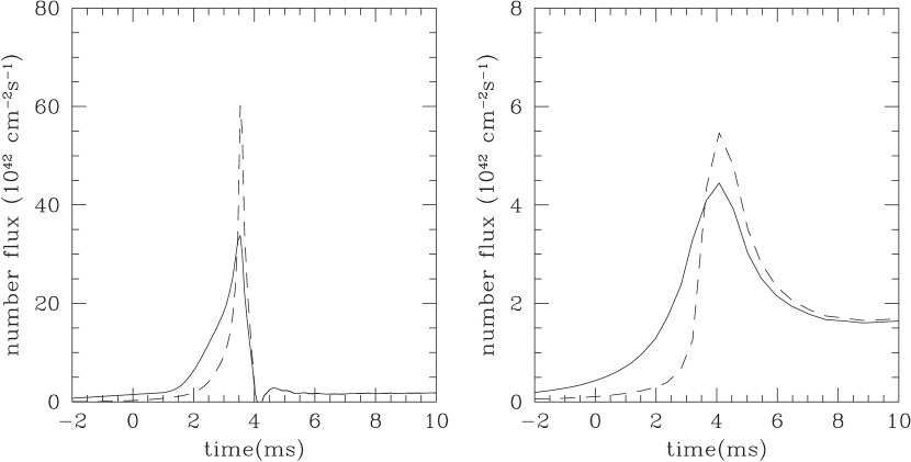
Figure 7: Time evolutions of the number flux for the electron-type neutrino with the energy $10~{}\mathrm{MeV}<E<20~{}\mathrm{MeV}$ detected by the comoving observer. Solid lines and dashed lines represent the results of our computation and the values estimated by the number density in equilibrium and $\langle\cos\theta\rangle$ of our computation, respectively. The left panel corresponds to model 1a ($s=3k_{\mathrm{B}}$) at $M=1.3M_{\odot}$ and the right to model 4a ($s=7.5k_{\mathrm{B}}$) at $M=3.3M_{\odot}$.

where $T$ and $\mu_{\nu}$ are the temperature and the chemical potential of the electron-type neutrino in $\beta$-equilibrium at the shock surface, respectively, and $k_{\mathrm{B}}$ is the Boltzmann constant. Here the value $\mu_{\nu}$ is defined as $\mu_{\nu}\equiv\mu_{e}-(\mu_{n}-\mu_{p})$, where $\mu_{e}$, $\mu_{n}$ and $\mu_{p}$ are the chemical potentials of electron, neutron and proton, respectively, and they are given in the equation of state by Shen et al. (1998a, 1998b). The number flux is estimated as $cn_{\mathrm{eq.}}\langle\cos\theta\rangle$, where $\langle\cos\theta\rangle$ is a mean value of the angular cosine over the neutrino angular distribution and $c$ is the light velocity. In Figure 7, we compare the results of our numerical computation with the number flux estimated above. We can see that the equilibrium is not achieved completely, but the fraction is rather constant, $\sim 0.6$. Therefore, the luminosity is well estimated by

$$L(\epsilon)d\epsilon=C\frac{16\pi^{2}r^{2}\langle\cos\theta\rangle\epsilon^{3}}{h^{3}c^{2}\left(\exp\left(\frac{\epsilon-\mu_{\nu}}{k_{\mathrm{B}}T}\right)+1\right)}d\epsilon,$$ (3)

where $h$ is the Planck constant, $r$ is the radius of the shock surface and $C\sim 0.6$.

From equation (3), we can see that the luminosity is determined by $r$, $\mu_{\nu}$, $T$ and $\langle\cos\theta\rangle$. According to our numerical computation, $T\sim 1.5$ MeV and $\langle\cos\theta\rangle\sim 0.5$ do not change very much on the time scale of the neutronization burst. Thus, the luminosity is dictated mainly by $r$ and $\mu_{\nu}$. Snapshots of the profiles of $\mu_{\nu}$ are shown in the lower left panel of Figure 6, and we can see that $\mu_{\nu}$ has a peak on the shock surface for the following reason. When matter accretes onto the shock, the baryon mass density and the electron number density rise, leading to the increase of $\mu_{e}$ and, as a result, $\mu_{\nu}$. Immediately thereafter, neutronization occurs and the value of $(\mu_{n}-\mu_{p})$ rises, which reduces $\mu_{\nu}$. We can recognize from Figure 6 that the peaks of $\mu_{\nu}$ and the luminosity are correlated. As for the time evolution, the luminosity on the shock surface is lower at the early phase because the shock radius is small. On the other hand, it is also lower at the late phase because $\mu_{\nu}$ is lower. This is the reason why the luminosity on the shock surface has a peak.

We now investigate model 4a, whose initial entropy is $s=7.5k_{\mathrm{B}}$. In the lower right panel of Figure 6, snapshots of the profiles of $\mu_{\nu}$ for model 4a are shown. We can see that the value of $\mu_{\nu}$ at the shock surface is lower than that of model 1a at the early phase. This is because the baryon mass density on the shock surface of model 4a at the bounce is lower than that of model 1a, as has been mentioned. Accordingly, the electron number density and $\mu_{e}$ are also lower for model 4a, and $\mu_{\nu}$ does not rise so high. This is the main reason why the neutronization burst is not remarkable. It is noted, moreover, that the electron fraction, $Y_{e}$, on the shock surface of model 4a is lower than that of model 1a. This is because nuclei do not exist and the nucleons are already neutronized on the shock surface. The absence of nuclei is consistent with the fact that the higher the initial entropy is, the earlier nuclei dissolve into nucleons, as explained by Figure 3. In addition, we can see that the luminosity of $\nu_{e}$ rises monotonically. This is because the area of a shock surface increases whereas $\mu_{\nu}$ is almost unchanging.

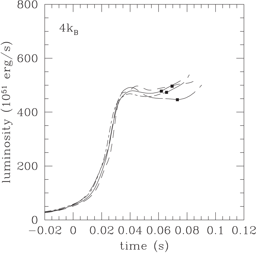
Figure 8: Luminosities of $\nu_{e}$ as a function of $t$ for models 2a (solid line), 2m (short-dashed line), 2e (long-dashed line) and 2g (dot-dashed line). The meaning of squares is the same as in Figure 5.

The results for the models with higher resolutions are shown in Figure 8. While the duration times of their neutrino emissions differ slightly among the models as mentioned already, the profiles of their neutronization bursts are not very different qualitatively. In fact, the luminosity declines a little after the peak and increases again for model 2a. This feature is well kept in other models with higher resolutions.

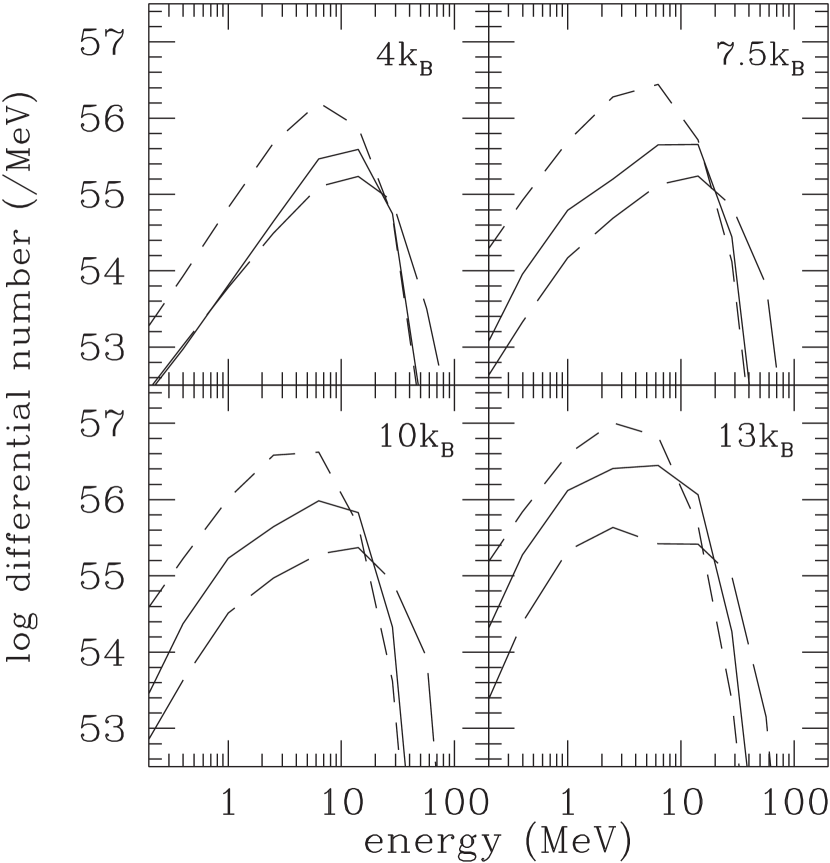
Figure 9: Spectra of time-integrated emissions of $\nu_{e}$ (short-dashed line), $\bar{\nu}_{e}$ (solid line) and $\nu_{x}$ (long-dashed line). Upper left, upper right, lower left and lower right panels are for models 2a ($s=4k_{\mathrm{B}}$), 4a ($s=7.5k_{\mathrm{B}}$), 5a ($s=10k_{\mathrm{B}}$) and 6a ($s=13k_{\mathrm{B}}$), respectively.

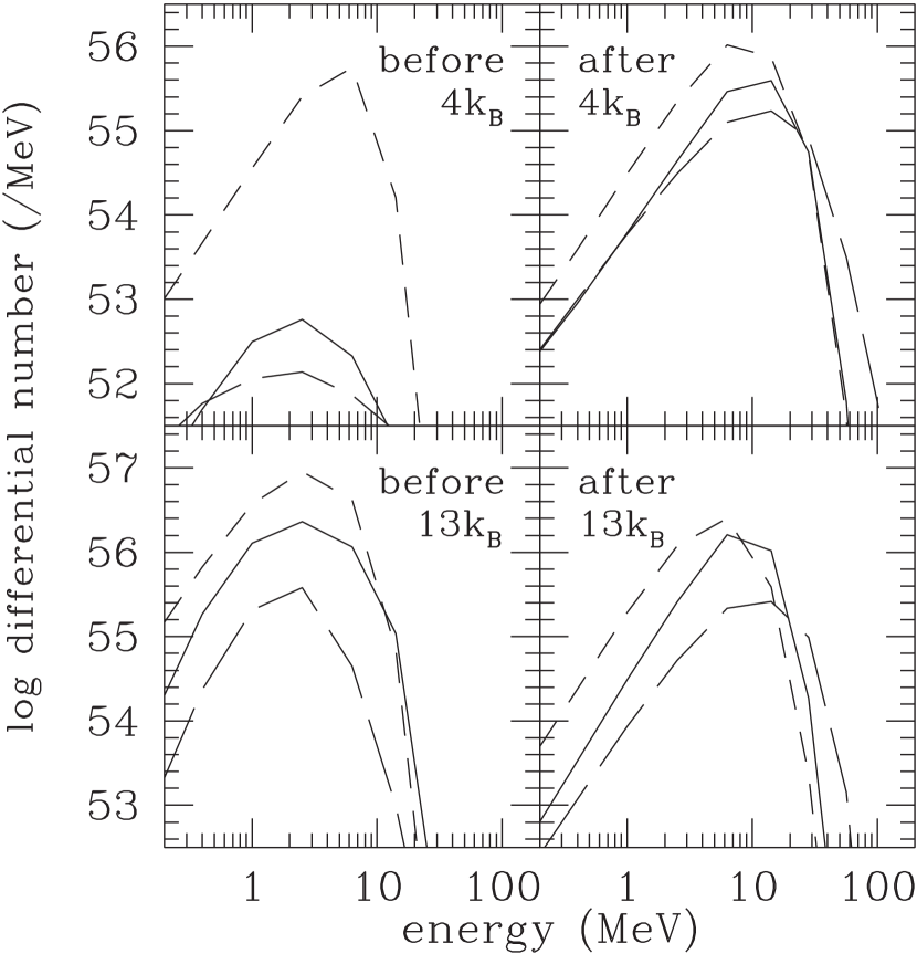
Figure 10: Spectra of time-integrated emissions of $\nu_{e}$ (short-dashed line), $\bar{\nu}_{e}$ (solid line) and $\nu_{x}$ (long-dashed line). The upper left and upper right panels give the time integrations of the emission before and after bounce, respectively, for model 2a ($s=4k_{\mathrm{B}}$). The lower left and lower right panels present the emission before and after shock formation, respectively, for model 6a ($s=13k_{\mathrm{B}}$).

We show the time-integrated neutrino spectra in Figure 9. We can see that the spectra become softer for higher entropy models, especially for $\bar{\nu}_{e}$ and $\nu_{x}$. In order to investigate this tendency, we show the time-integrated spectra of the neutrino emitted before and after the shock formation in Figure 10. We can see that, for higher entropy models, $\bar{\nu}_{e}$ and $\nu_{x}$ are also emitted before the shock formation. They are created by the electron-positron pair annihilation, and their energy is relatively lower ($\lesssim$ several MeV) because the temperature is low ($T\lesssim 1$ MeV). On the other hand, for lower entropy models, $\bar{\nu}_{e}$ and $\nu_{x}$ can not be produced by the electron-positron pair process because positrons are absent owing to Pauli blocking. As for the $\bar{\nu}_{e}$ and $\nu_{x}$ emitted after the shock formation, they are mainly created by bremsstrahlung. In this phase, the temperature near the neutrino sphere rises to $T\sim$ several MeV, which makes the neutrino energies relatively high: $\sim 10$ MeV. Since the low energy ($\lesssim$ several MeV) neutrinos are not emitted to any great extent and the spectra become harder for lower entropy models, the emission of low energy $\bar{\nu}_{e}$ and $\nu_{x}$ is characteristic for the collapse of high entropy cores.

3.3 Initial Velocity Dependence

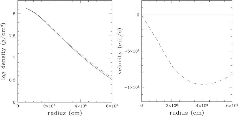
Figure 11: Comparisons of the density profiles (left) and the velocity profiles (right). Solid lines represent the initial profiles for model 2a; dashed lines represent the profiles for model 2b at the time when the central density becomes the same as the initial central density of model 2a.

We compare the results of models 2a and 2b, which are different in the initial values of central density and temperature, but have the same initial values of entropy per baryon ($s=4k_{\mathrm{B}}$). We can consider that models 2a and 2b are the same model but with different initial velocities, because the density profile of model 2b at the time when the central density reaches that of the initial model of 2a almost coincides with that of model 2a (Figure 11). In reality, the onset of a collapse is determined not only by the core structure but also by the whole stellar structure. Thus, studying the initial velocity dependence of the core is meaningful.

As a result of this comparison, we find that the initial velocity does not affect crucially the ensuing dynamics and the features of emitted neutrinos such as total number spectra or the time evolutions of the luminosity. This is because the velocity of model 2b at the time in Figure 11 is several times lower than the sound speed at each point. For instance, the fastest point of model 2b in Figure 11 has the velocity $\sim 10^{8}\mathrm{cm\,\mathrm{s}^{-1}}$ while the sound speed is $\sim 7\times 10^{8}\mathrm{cm\,\mathrm{s}^{-1}}$, there. If the supersonic region, where the infalling velocity exceeds the sound speed, existed in the initial model, the initial velocity profile may be important for the dynamics. However, since the temperature of our initial models is slightly higher than the critical temperature for the photodisintegration instability, they are unlikely to have supersonic region.

3.4 Collapse of Population III Star with $100M_{\odot}$

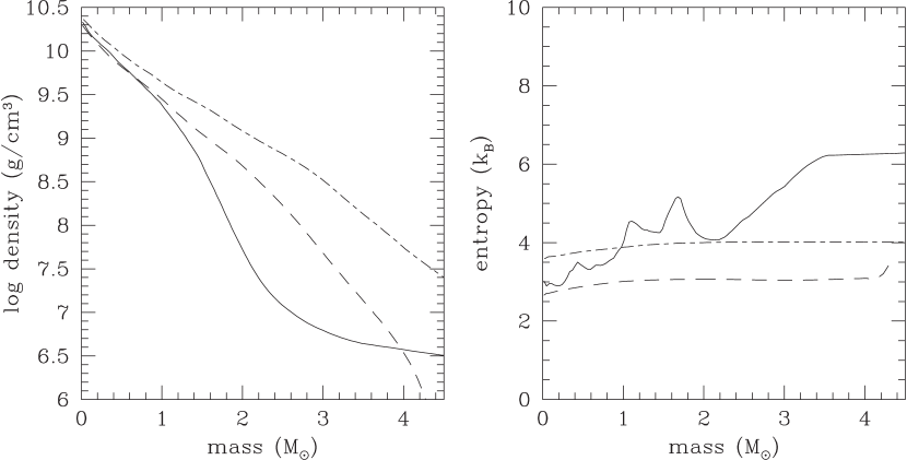
Figure 12: Comparisons of the density profiles (left) and the entropy profiles (right). Solid lines represent the initial profiles for model R and dashed and dot-dashed lines represent the profiles for models 1a and 2a, respectively, at the time when the central density becomes the same as the initial central density of model R.

In this section, we consider yet another example of very massive stars, that is, a Population III star with $100M_{\odot}$. We use a model constructed by Nomoto et al. (2005) with evolutionary calculations, and we refer to it as model R. This model is very massive and its entropy at the center is higher than that of ordinary supernova progenitors when it starts to collapse because the star does not lose its mass at all in its evolution owing to its zero metallicity. It should be emphasized that the isentropic models are meant for the massive stars that may be produced in the present universe, for example, by stellar mergers in clusters whereas Model R corresponds to a first-generation star in the past universe. Here we are interested in the differences that these models may make. In Figure 12, we show the comparison of the initial state of model R and our isentropic models at the time when their central densities become the same as that of model R. We can recognize that model R has the entropy $\sim 3.5k_{\mathrm{B}}$ in the central region, which is between those of model 1a and 2a, whereas the iron core of model R is smaller than that of our models. In fact, the iron core mass of model R is $\sim 2.32M_{\odot}$, which is close to that of model 1a. We show some of the initial values at the center of model R in Table 1. Incidentally, the initial velocity profile is taken into account for model R although it is much lower than the sound speed at each point.

As a result of collapse, model R has a bounce and recollapses to a black hole. As shown in Table 1, the values of the central density and the central adiabatic index of model R at the bounce are between those of model 1a and 2a. This suggests that these values are determined by the initial central entropy as mentioned in § 3.1. On the other hand, model R has a much longer time interval from the bounce to the recollapse, compared with our models. This is because the inner core mass of model R at the bounce ($M_{\mathrm{bounce}}$) is smaller and the lower density of the outer core (Figure 12) gives lower accretion rates. For instance, at $t=0.06$ s, model R has a mass accretion rate $\sim 4M_{\odot}\,\mathrm{s}^{-1}$ at the shock surface whereas model 1a has $\sim 11M_{\odot}\,\mathrm{s}^{-1}$. Thus it takes much time until the inner core mass exceeds the maximum mass of the neutron star.

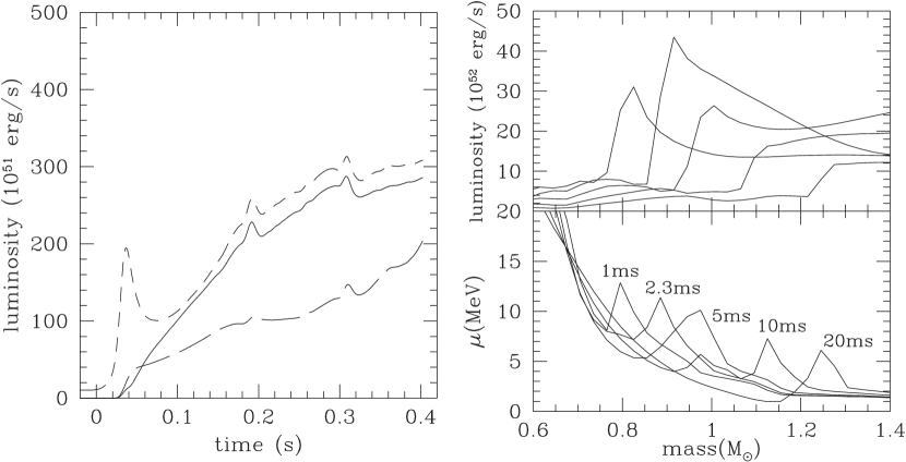
Figure 13: Results of the collapse for model R. In the left and right panel, the notations of lines are the same as in Figures 5 and 6, respectively, but the end points of the lines in the left panel represent the time when the apparent horizon is formed.

We show the total energy of neutrinos emitted during the collapse of model R in Table 2 and the time evolution of the emitted neutrino luminosity in Figure 13. We can see that the total energy of emitted neutrinos is larger than that of other isentropic models, despite the fact that the neutrino luminosity of model R is lower than those of our models. This is because model R neutrino emission lasts much longer. Moreover, the mean energy of the emitted neutrinos is larger for model R. This is also due to the longer duration time. The neutrino spectrum gets harder in the late phase because the density of the accreting matter becomes lower and the temperature on the neutrino sphere gets higher. Thus, the longer the duration time of neutrino emission is, the larger the mean energy of the emitted neutrinos becomes. It is noted that the duration time is sensitive to the equation of state, which is already mentioned, and hence the total and mean energy of emitted neutrinos is also sensitive to the equation of state.

In the following, we discuss the features of the emitted neutrinos from model R for the early phase, which is not sensitive to the equation of state as already mentioned. Comparing Figures 5 and 13, we can see that for model R, the peak luminosity of the electron-type neutrino by the neutronization burst is lower than those of our models. The reason why it is lower than that of model 1a ($s=3k_{\mathrm{B}}$) is because the chemical potential of an electron-type neutrino for model R is lower than that for model 1a, while the shock radii in both models are not so different from each other (right panels of Figure 13). It is consistent with the fact that the density at the bounce of model R is lower than that of model 1a (Table 1). On the other hand, the shock radii of models with $s\geq 4k_{\mathrm{B}}$ (models 2a-4a) are larger than that of model R. This is the reason why the luminosity of the neutronization burst for model R is lower than those of models 2a-4a. Furthermore, since the outer core density of model R is much lower than those of isentropic models (Figure 12), $\mu_{\nu}$ drops quickly and the shock radius does not get much larger after the neutronization. From equation (3), These features lead to the fact that the luminosity of the electron-type neutrino after the neutronization burst drops more steeply for model R than for our models. It follows, then, that the decline of the neutronization burst depends not only on the initial entropy but also on the initial density profile. In particular, the larger the initial density gradient is, the more steeply the neutronization burst declines.

To sum up, the key parameters listed in Table 1 at bounce (e.g. central density, temperature etc.) do not differ very much between the isentropic models and model R. This is not true for the time profile of the neutronization burst because they depend not only on the central density at bounce but also on the initial density profile. However, since, in general, more massive iron cores have larger entropies, the following trend is generally true: The neutronization burst will become less remarkable as the progenitor gets more massive.

3.5 Astrophysical Implications

3.5.1 Progenitor of IMBH

For supermassive black holes (SMBH) located at the center of many galaxies including ours, a new formation scenario via intermediate-mass black holes (IMBH) has recently been suggested (e.g., Ebisuzaki et al. 2001, Portegies Zwart et al. 2006). According to this scenario, very dense stellar clusters are initially formed in the vicinity of the galactic center ($\lesssim 10$ pc), and the massive stars with $\sim 20M_{\odot}$ in them undergo runaway collisions to form IMBHs before they lose most of their mass by supernova explosions and/or pulsations. After that, these IMBHs merge together and finally form SMBH. This scenario is supported by the discovery of the ultra luminous X-ray compact sources in M82 galaxy, which indicate the existence of IMBHs. It is conceivable that similar events occur in the Milky Way Galaxy as mentioned later. This scenario assumes that the supermassive stars formed by the runaway collisions would collapse to IMBHs when they are $\sim 1000M_{\odot}$.

Recently Suzuki et al. (2007) have studied the structures and evolutions of these merged stars in the hydrogen burning. According to them, the smaller star sits at the center of the larger star after the merger of two stars with different masses. It is also demonstrated that the merged stars become convectively unstable by the positive gradient of the mean molecular weight and that their evolutions thereafter approach those of the single homogeneous star with the same mass and abundance. The central entropies of the merged stars will then be larger than those of the inhomogeneous single stars with the same mass. This suggests the possibility to form the IMBH progenitors by the merger without experiencing the pair instability. Here we speculate the entropy of these stars using previous studies on the single Population III stars. Since the iron core of the Population III star with $100M_{\odot}$ has entropy of $\sim 3.5k_{\mathrm{B}}$ (Nomoto et al. 2005), it is expected that these IMBH progenitors have entropies $\gtrsim 3k_{\mathrm{B}}$.

Even if the pair instability occurs, the massive stars corresponding to our models may still be formed. In fact, the positive entropy gradient and/or rotation may suppress the convection in the merged star and the entropy at the center may remain low after the merge. Then the merged star has a massive envelope with a smaller core than the single stars with the same total mass. If the pair instability occurs for these objects, the nuclear burning may not produce total disruptions but lead to the eventual collapse. Again inferring from single Population III stars, we speculate that the central entropies of the merged stars will be smaller than $s\sim 16k_{\mathrm{B}}$, which corresponds to $300M_{\odot}$ in NSY06. It is incidentally mentioned that the relations between the total mass and the iron core mass of merged IMBH progenitors is highly uncertain at present.

In the preceding sections, we have shown that the neutrino signals from the black hole formation are sensitive to the inner region of the progenitor. In this section, assuming our models correspond to above-mentioned merged stars which collapse to IMBHs at the center of our Galaxy ($\sim 8.5$ kpc from the sun), we estimate the neutrino event number for the currently operating detectors.

As for the event rate of the IMBH formation, based on the above-mentioned scenario and the fact that the SMBH residing in the center of our Galaxy (SgrA^∗) is $\sim 3.5\times 10^{6}M_{\odot}$ and the age of our Galaxy is $\sim 10$ Gyr, a very rough estimation for the formation rate of IMBH with $\sim 1000M_{\odot}$ is $\lesssim$ once per 1 Myr. It is, however, mentioned that this event rate may be underestimated because star formation may not be continuous but triggered by some environmental effects (e.g., the merger of galaxies). Recent observations by Paumard et al. (2006) have revealed the existence of about 80 young massive stars within a distance of a parsec from SgrA^∗ and some of them are identified as OB stars and their ages are about $6\pm 2$ Myr. These facts indicate that stars are actively formed in this region at present. Moreover, the IMBH candidate with $\sim 1300M_{\odot}$, IRS 13, is found in the same region (Maillard et al. 2004). Thus, SgrA^∗ may be currently growing under this scenario.

In the following estimations for the neutrino event number, we do not take into account the neutrino mixing, although it should be. Since the mixing occurs mainly in the resonance regions and they are located outside the iron core of the progenitor, the neutrino oscillation does not affect the dynamics of core. Unfortunately the structures of the envelopes of merged stars, which are crucial for the neutrino mixing, are quite uncertain. There remain uncertainties as well on the mixing parameters, such as the mixing angle of $\sin^{2}2\theta_{13}$ or the mass hierarchy. Thus, the precise evaluation of the neutrino flux including the neutrino mixing is deferred to future study.

3.5.2 Detection of low energy $\bar{\nu}_{e}$ by Super Kamiokande and KamLAND

As already mentioned, a good deal of low energy $\bar{\nu}_{e}$ is emitted from the collapse of the high entropy cores, which softens the spectrum. We estimate the $\bar{\nu}_{e}$ event number for Super Kamiokande III and KamLAND, currently operating neutrino detectors, under the assumption that the black hole formations considered in former sections occur at the center of our Galaxy. For both detectors, the dominant reaction is the inverse beta decay,

$$\bar{\nu}_{e}+p\longrightarrow e^{+}+n,$$ (4)

which we take into account only. We adopt the cross section for this reaction from Vogel & Beacom (1999). For Super Kamiokande III, we assume that the fiducial volume is 22.5 kton and the trigger efficiency is 100% at 4.5 MeV and 0% at 2.9 MeV, which are the values at the end of Super Kamiokande I (Hosaka et al. 2006). For KamLAND, we assume 1 kton fiducial mass, which means that $8.48\times 10^{31}$ free protons are contained (Eguchi et al. 2003). We also assume that the trigger efficiency is 100% for all $\bar{\nu}_{e}$ energy larger than the threshold energy of the reaction.

The results are given in Table 3. The total event number does not change monotonically with the initial entropy of the core because the total number of neutrinos depends on both the core mass and the duration time of neutrino emission, as already mentioned. In order to investigate the hardness of $\bar{\nu}_{e}$ spectrum, we calculate the ratio of the event number by $\bar{\nu}_{e}$ with $<10$ MeV to that for all events. The ambiguity about the distance of source is also canceled by this normalization. This ratio gets larger as the entropy of the core becomes higher. This suggests that we can probe the entropy of the black hole progenitor especially in higher regimes ($s\geq 7.5k_{\mathrm{B}}$) because the event numbers of $\bar{\nu}_{e}$ with $<10$ MeV are over 100 by Super Kamiokande III.

3.5.3 Detection of neutronization burst by SNO

The SNO detector consists of 1 kton of pure heavy water (D₂O) and can distinguish $\nu_{e}$ flux by the charged-current reaction of the deuterium disintegration. Since SNO can also detect the $\bar{\nu}_{e}$ flux, we can estimate the intensity of the neutronization burst by comparing the event from the charged-current reaction of $\nu_{e}$,

$$\nu_{e}+d\longrightarrow p+p+e^{-},$$ (5)

and that of $\bar{\nu}_{e}$,

$$\bar{\nu}_{e}+d\longrightarrow n+n+e^{+},$$ (6)

using the SNO detector. SNO can also detect the neutral-current reaction,

$$\nu+d\longrightarrow n+p+\nu,$$ (7)

for all species. It is noted that the neutral-current reaction contains $\nu_{x}$ ($=\nu_{\mu}$, $\bar{\nu}_{\mu}$, $\nu_{\tau}$ and $\bar{\nu}_{\tau}$) and the neutrino sphere of $\nu_{x}$ differs more from that of $\nu_{e}$ than that of $\bar{\nu}_{e}$ in general. Thus, for the comparison with reaction (5), reaction (6) is more appropriate than reaction (7). On the other hand, we also use (7) for the comparison because the event number of (7) is larger than that of (6). In our calculation, we use the cross sections from Ying et al. (1989) and assume that the trigger efficiency of these reactions is 100%. In fact, it is $\sim$ 92% these days, which is the neutron (in the right hand side of equation (7)) capture efficiency on ³⁵Cl and deuterons (Oser 2005).

In the following analysis, we regard the emission of neutrinos before $t=0.06$ s as the neutronization burst, where the time $t$ is measured from the bounce. The criterion $t=0.06$ s is chosen empirically from our simulations as an expedient. The method for extracting the neutronization burst from detection should be reconsidered for more detailed studies. Here we calculate the event numbers for $t<0.06$ s as well as those for the entire duration time of the neutrino emission, and the results are summarized in Table 4. We can recognize that the ratios of the $\nu_{e}$ event number ($N_{\nu_{e},<0.06\,\mathrm{s}}$) to the total event number of the charged-current reactions ($N_{\nu_{e},<0.06\,\mathrm{s}}+N_{\bar{\nu}_{e},<0.06\,\mathrm{s}}$) and that for the neutral-current reaction ($N_{NC,<0.06\,\mathrm{s}}$) are larger for the models whose neutronization burst declines more steeply. Despite the fact that these neutronization burst numbers are of the order of 10, we can probe into the black hole progenitors in principle.

It is finally noted that the estimations in the current study are based on the spherically symmetric models. If progenitors are rotating rapidly, the neutrino sphere will become non-spherical and the neutrino emissions will be affected in general. This will be the subject of future investigations.

4 Conclusions

In this paper, we have numerically studied gravitational collapse and black hole formation of massive iron cores systematically, taking into account the reactions and transports of neutrinos in detail. Massive iron cores with $\sim 10M_{\odot}$ have a bounce owing to thermal nucleons, following which they collapse to black holes when the maximum mass is reached. As for the emitted neutrinos, the spectra of $\bar{\nu}_{e}$ and $\nu_{x}$ ($=\nu_{\mu}$, $\bar{\nu}_{\mu}$, $\nu_{\tau}$ and $\bar{\nu}_{\tau}$) become softer for more massive models, or higher entropy models, because a high entropy generates a large number of electron-positron pairs, which create $\bar{\nu}_{e}$ and $\nu_{x}$. The neutronization burst from more massive iron core becomes less remarkable or disappears completely. This is because the density at the bounce is lower and even the $\nu_{e}$ number density in equilibrium becomes lower.

We have found that if the initial velocity is lower than the sound speed, it does not affect the collapse very much. We have also compared the collapse of our isentropic models with that of the realistic model, which is obtained by the detailed modeling of the evolution of Population III stars and we have found that the steep decline of the neutronization burst depends not only on the initial entropy but also on the initial density profile. Moreover, assuming our models as the progenitors of IMBHs collapsing at the Galactic center, we have estimated the neutrino event numbers. As a result, for Super Kamiokande III, the ratio of the $\bar{\nu}_{e}$ event number for $<10$ MeV to that for all events gets larger as the entropy of the core becomes higher, especially for $s\geq 7.5k_{\mathrm{B}}$. We have suggested that we can use these features to probe into the progenitors. As for the lower entropy cores, despite the fact that the event number for the early phase of the emission is less than 100 by SNO, we have suggested that the steep decline of the neutronization burst can be distinguished in principle.

Concerning the prediction of neutrino event number, there is a room for further improvement. Firstly, the effects of the neutrino oscillation should be taken into account. Secondly, multi-dimensional effects, such as rotation or magnetic field may be important, since they will affect the dynamics of collapse itself. This study will be hopefully prove a first step toward a neutrino astrophysics for black holes.

Table 1: Key Parameters for all Models.

	$s_{\mathrm{initial}}$	$M_{\mathrm{iron}}$	$\rho_{\mathrm{initial}}$	$T_{\mathrm{initial}}$	$M_{\mathrm{bounce}}$	$\rho_{\mathrm{bounce}}$	$T_{\mathrm{bounce}}$	$\gamma_{\mathrm{bounce}}$	$t_{\mathrm{recollapse}}$
model	($k_{\mathrm{B}}$)	($M_{\odot}$)	($\mathrm{g\,cm^{-3}}$)	(K)	($M_{\odot}$)	($\mathrm{g\,cm^{-3}}$)	(MeV)		(msec)
1a	3.0	2.44	2.71$\times 10^{8}$	7.75$\times 10^{9}$	0.75	1.95$\times 10^{14}$	25.9	2.38	96.7
2a	4.0	3.49	1.40$\times 10^{8}$	7.75$\times 10^{9}$	1.10	9.58$\times 10^{13}$	26.9	1.89	62.0
2b	4.0	2.93	7.00$\times 10^{7}$	6.86$\times 10^{9}$	1.05	9.90$\times 10^{13}$	26.7	1.91	63.4
3a	5.0	4.97	8.82$\times 10^{7}$	7.75$\times 10^{9}$	1.5	2.97$\times 10^{13}$	19.4	1.58	52.6
4a	7.5	10.6	4.20$\times 10^{7}$	7.75$\times 10^{9}$	2.7	3.00$\times 10^{12}$	12.0	1.54	37.9
5a	10.0	19.3	2.67$\times 10^{7}$	7.75$\times 10^{9}$	—	—	—	—	—
6a	13.0	34.0	1.84$\times 10^{7}$	7.75$\times 10^{9}$	—	—	—	—	—
R	3.5	2.32	2.34$\times 10^{10}$	1.61$\times 10^{10}$	0.65	1.37$\times 10^{14}$	22.7	2.19	402
2a	4.0	3.49	1.40$\times 10^{8}$	7.75$\times 10^{9}$	1.10	9.58$\times 10^{13}$	26.9	1.89	62.0
2m	4.0	3.49	1.40$\times 10^{8}$	7.75$\times 10^{9}$	1.04	9.64$\times 10^{13}$	27.5	1.88	69.5
2g	4.0	3.49	1.40$\times 10^{8}$	7.75$\times 10^{9}$	1.05	9.66$\times 10^{13}$	27.2	1.88	65.7
2e	4.0	3.49	1.40$\times 10^{8}$	7.75$\times 10^{9}$	1.10	8.25$\times 10^{13}$	25.9	1.80	73.2

Table 2: Estimates of Average and Total Energies of Emitted Neutrinos.

	$\langle{E_{\nu_{e}}\rangle}$	$\langle{E_{\bar{\nu}_{e}}\rangle}$	$\langle{E_{\nu_{x}}\rangle}$	$E^{\mathrm{tot}}_{\nu_{e},52}$	$E^{\mathrm{tot}}_{\bar{\nu}_{e},52}$	$E^{\mathrm{tot}}_{\nu_{x},52}$	$E^{\mathrm{tot}}_{\mathrm{all},52}$
model	(MeV)	(MeV)	(MeV)	($10^{52}\mathrm{ergs}$)	($10^{52}\mathrm{ergs}$)	($10^{52}\mathrm{ergs}$)	($10^{52}\mathrm{ergs}$)
1a	11.01 - 11.01	15.03 - 15.03	19.60 - 19.60	3.29 - 3.29	1.94 - 1.94	1.43 - 1.43	10.96 - 10.96
2a	10.32 - 10.32	14.29 - 14.30	19.30 - 19.30	3.21 - 3.21	1.58 - 1.58	1.33 - 1.33	10.12 - 10.12
2b	10.17 - 10.17	14.27 - 14.27	19.35 - 19.35	3.24 - 3.24	1.63 - 1.63	1.36 - 1.36	10.29 - 10.29
3a	9.29 - 9.29	13.79 - 13.79	19.31 - 19.31	3.10 - 3.10	1.48 - 1.48	1.30 - 1.30	9.78 - 9.78
4a	7.30 - 7.30	11.95 - 11.95	19.55 - 19.55	3.19 - 3.19	1.56 - 1.56	1.35 - 1.36	10.18 - 10.21
5a	6.24 - 6.25	10.34 - 10.37	18.37 - 18.70	4.01 - 4.02	2.34 - 2.35	1.69 - 1.73	13.11 - 13.31
6a	5.24 - 5.25	8.14 - 8.19	14.33 - 14.33	6.15 - 6.17	4.71 - 4.75	1.70 - 1.73	17.66 - 17.84
R	15.34 - 15.34	18.90 - 18.90	23.42 - 23.42	9.42 - 9.42	7.89 - 7.89	4.40 - 4.40	34.89 - 34.90

Note. — $s_{\mathrm{initial}}$ is the initial value of the entropy par baryon. $M_{\mathrm{iron}}$ and $M_{\mathrm{bounce}}$ are the mass of initial iron core and inner core at the bounce ($t=0$), respectively. $\rho_{\mathrm{initial}}$ and $\rho_{\mathrm{bounce}}$ are the central density of the initial model and at the bounce, respectively. $T_{\mathrm{initial}}$ and $T_{\mathrm{bounce}}$ are the central temperature of the initial model and at the bounce, respectively. $\gamma_{\mathrm{bounce}}$ is the central adiabatic index at the bounce. $t_{\mathrm{recollapse}}$ is the interval time from the bounce to the apparent horizon formation.

Note. — The mean energy of emitted $\nu_{i}$ (with upper and lower limits) is denoted as $\langle{E_{\nu_{i}}\rangle}\equiv E^{\mathrm{tot}}_{\nu_{i}}/N^{\mathrm{tot}}_{\nu_{i}}$, where $E^{\mathrm{tot}}_{\nu_{i}}$ and $N^{\mathrm{tot}}_{\nu_{i}}$ are the total energy and number of neutrinos. $E^{\mathrm{tot}}_{\mathrm{all}}$ is the total energy summed over all species.

Table 3: Event Numbers of $\bar{\nu}_{e}$ from Super Kamiokande III and KamLAND.

model	$\frac{N_{\bar{\nu}_{e}<\mathrm{10\,MeV,SK}}}{N_{\bar{\nu}_{e},\mathrm{SK}}}$	$N_{\bar{\nu}_{e},\mathrm{SK}}$	$\frac{N_{\bar{\nu}_{e}<\mathrm{10\,MeV,Kam}}}{N_{\bar{\nu}_{e},\mathrm{Kam}}}$	$N_{\bar{\nu}_{e},\mathrm{Kam}}$
1a	3.3%	6163	3.3%	174
2a	4.0%	4778	4.0%	135
2b	4.0%	4910	4.0%	139
3a	4.6%	4319	4.6%	122
4a	7.3%	4018	7.3%	114
5a	11.8%	5326	12.0%	151
6a	20.1%	9139	20.5%	259

Table 4: Event Numbers by SNO.

model	$N_{\nu_{e},<0.06\,\mathrm{s}}$	$N_{\bar{\nu}_{e},<0.06\,\mathrm{s}}$	$\frac{N_{\nu_{e},<0.06\,\mathrm{s}}}{N_{\nu_{e},<0.06\,\mathrm{s}}+N_{\bar{\nu}_{e},<0.06\,\mathrm{s}}}$	$N_{\mathrm{NC,}<0.06\,\mathrm{s}}$	$\frac{N_{\mathrm{\nu_{e},}<0.06\mathrm{s}}}{N_{\mathrm{NC,}<0.06\,\mathrm{s}}}$	$N_{\mathrm{\nu_{e},all}}$	$N_{\mathrm{\bar{\nu}_{e},all}}$	$N_{\mathrm{NC,all}}$
1a	30.7	6.4	82.7%	45.4	67.5%	84.2	45.4	201
2a	40.8	10.7	79.2%	70.4	57.9%	69.8	30.1	162
2b	42.6	12.4	77.5%	77.1	55.3%	73.6	33.8	179
3a	38.4	12.6	75.3%	78.5	49.0%	56.7	24.7	142
4a	31.8	15.1	67.9%	91.2	34.9%	37.4	19.3	124
5a	—	—	—	—	—	44.9	32.7	220
6a	—	—	—	—	—	59.3	54.0	221

Note. — The subscript“$<10$ MeV” means the event of $\bar{\nu}_{e}$ with $<10$ MeV, and the subscript “SK” and “Kam” mean the prediction for Super Kamiokande III and KamLAND, respectively.

Note. — These values are the event number for the charged-current reaction except $N_{\mathrm{NC,}<0.06\mathrm{s}}$ and $N_{\mathrm{NC,all}}$. The subscript“$<0.06$ s” means the event at $t<0.06$ s, where $t$ is the time measured from the bounce, and the subscript “all” means the event for all duration times of neutrino emission.

References

- (1) Ebisuzaki, T., et al. 2001, ApJ, 562, L19
- (2) Eguchi, K., et al. 2003, Phys. Rev. Lett., 90, 021802
- (3) Fryer, C. L. 1999, ApJ, 522, 413
- (4) Fryer, C. L., Woosley, S. E., & Heger, A. 2001, ApJ, 550, 372
- (5) Heger, A., Fryer, C. L., Woosley, S. E., Langer, N & Hartmann, D. H. 2003, ApJ, 591, 288
- (6) Herant, M., Benz, W., Hix, W. R., Fryer, C. L., & Colgate, C. A. 1994, ApJ, 435, 339
- (7) Hosaka, J., et al. 2006, Phys. Rev. D, 73, 112001
- (8) Linke, F., Font, J. A., Janka, H.-Th., Mller, E., & Papadopoulos, P. 2001, A&A, 376, 568
- (9) Maillard, J. P., Paumard, T., Stolovy, S. R., & Riguaut, F. 2004, A&A, 423, 155
- (10) Misner, C. W., & Sharp, D. H. 1964, Phys. Rev., 136, 571
- (11) Nakamura, F., & Umemura, M. 2001, ApJ, 548, 19
- (12) Nakazato, K., Sumiyoshi, K., & Yamada, S. 2006, ApJ, 645, 519
- (13) Nomoto, K., Tominaga, N., Umeda, H., Maeda, K., Ohkubo, T., Deng, J., & Mazzali, P. A. 2005, ASP Conf. Ser., 332, 374
- (14) Ohkubo, T., Umeda, H., Maeda, K., Nomoto, K., Tsuruta, S., & Rees, M. J. 2006, ApJ, 645, 1352
- (15) Oser, S. M. 2005, Nucl. Phys., A758, 677c
- (16) Paumard, T., et al. 2006, ApJ, 643, 1011
- (17) Portegies Zwart, S. F., Makino, J., McMillian, S. L. W., & Hut, P., 1999, A&A, 348, 117
- (18) Portegies Zwart, S. F., Baumgardt, H., McMillian, S. L. W., Makino, J., Hut, P., & Ebisuzaki, T. 2006, ApJ, 641, 319
- (19) Sekiguchi, Y. I., & Shibata, M. 2005, Phys. Rev. D, 71, 084013
- (20) Shen, H., Toki, H., Oyamatsu, K., & Sumiyoshi, K. 1998a, Nucl. Phys., A637, 435
- (21) Shen, H., Toki, H., Oyamatsu, K., & Sumiyoshi, K. 1998b, Prog. Theor. Phys., 100, 1013
- (22) Sumiyoshi, K., Yamada, S., Suzuki, H., Shen, H., Chiba, S., & Toki, H. 2005, ApJ, 629, 922
- (23) Sumiyoshi, K., Yamada, S., Suzuki, H., & Chiba, S., 2006, Phys. Rev. Lett., 97, 091101
- (24) Suzuki, T. K., Nakasato, N., Baumgardt, H., Ibukiyama, A., Makino, J., & Ebisuzaki, T. 2007, astro-ph/0703290, submitted to ApJ
- (25) Thompson, T. A., Burrows, A., & Pinto, P. A. 2003, ApJ, 592, 434
- (26) van Riper K. A. 1979, ApJ, 232, 558
- (27) Vogel, P., & Beacom, J. F. 1999, Phys. Rev. D, 60, 053003
- (28) Yamada, S. 1997, ApJ, 475, 720
- (29) Yamada, S., Janka, H.-Th., & Suzuki, H. 1999, A&A, 344, 533
- (30) Ying, S., Haxton, W. C., & Henley, E. M. 1989, Phys. Rev. D, 40, 3211