Macroscopic Greenberger-Horne-Zeilinger and W States in Flux Qubits

Abstract

We investigate two types of genuine three-qubit entanglement, known as the Greenberger-Horne-Zeilinger(GHZ) and W states, in a macroscopic quantum system. Superconducting flux qubits are considered theoretically in order to generate such states. A phase coupling is proposed to offer enough strength of interactions between qubits. While an excited state can be the W state, the GHZ state is formed at the ground state of the three flux qubits. The GHZ and W states are shown to be robust against external flux fluctuations for feasible experimental realizations.

Introduction.$-$Entanglement plays a crucial role in quantum information science. Controllable quantum systems such as photons, atoms, and ions have provided the opportunities to generate the entanglements. Recent experiments on two qubits have shown the existence of entanglement in different types of microscopic systems. Further, multipartite entanglements such as the Greenberger-Horne-Zeilinger(GHZ) Greenberger and W Zeilinger92 ; Dur states have been demonstrated in recent experiments of atoms Rau , photons and trapped ions Bouwmeester ; Roos . But, in solid-state qubits it has not yet been achieved.

As a macroscopic quantum system, superconducting qubit systems have been investigated intensively in experiments because their system parameters can be controlled to manipulate quantum states coherently. Indeed, the entanglements between two charge Pashkin , phase Berkley ; Steffen , and flux qubits Izmalkov ; Plant have been reported. While the timely evolving states in the experiments of charge qubits Pashkin exhibit a partial entanglement, the excited level (eigenstate) of capacitively coupled two phase qubits Steffen shows higher fidelity for the entanglement. The experiments in Ref. Izmalkov show a possibility that two flux qubits can be entangled by a macroscopic quantum tunneling between two-qubit states, flipping both qubits. Actually, the higher fidelity in the capacitively coupled two phase qubits is caused by the two-qubit tunneling processes Steffen . In a very recent study, the two-qubit tunneling process was theoretically shown to play an important role in generating the Bell states, maximally entangled, in the ground and excited states KimCho .

For multipartite entanglements in superconducting qubit systems, there have been few studies. To produce the GHZ state in three charge qubits, only a way of doing a local qubit operation via time evolutions was suggested Wei . As one of possible directions to produce such multipartite entanglements, then, it is natural to ask how to create the W state as well as the GHZ state in the eigenstates of superconducting three-qubit systems. Here we consider three flux qubits. Normally, the interaction strength between inductively coupled flux qubits Majer is not so strong that the controllable range of interaction is not sufficiently wide. To control a wide range of interaction strengths in the qubits, we use the phase-coupling scheme KimTwo ; Ploeg ; KimCont ; Grajcar ; Cho07 for three qubit (see Fig. 1(a)) which enables to generate the GHZ and W states and to keep them robust against external flux fluctuations for feasible experimental realizations.

Model.$-$We start with the model shown in Fig. 1(a). The Hamiltonian is written by $\hat{H}=\frac{1}{2}\hat{P}^{T}_{i}{M}^{-1}_{ij}\hat{P}_{j}+U_{\rm eff}(\hat{\bm{\phi}}),$ where $\hat{P}_{i}=-i\hbar\partial/\partial\hat{\phi}_{i}$ and $M_{ij}=(\Phi_{0}/2\pi)^{2}C_{i}\delta_{ij}$ with the capacitance of the Josephson junctions $C_{i}$. The dynamics of the flux qubits Mooij are described by the phase variables $\hat{\bm{\phi}}=(\phi_{qi},\phi^{\prime}_{q})$ with $q=a,b,c$ and $i=1,2,3$, where $\phi$’s are the phase differences across the Josephson junctions. If we neglect the small inductive energy, the effective potential is written in terms of the Josephson junction energies, $U_{\rm eff}(\bm{\phi})=\sum_{q}[\sum^{3}_{i=1}E_{Ji}(1-\cos\phi_{qi})+E^{\prime}_{J}(1-\cos\phi^{\prime}_{q})]$. The periodic boundary conditions involved in the qubit loops and the connecting loops can be written as

$$\phi_{q1}+\phi_{q2}+\phi_{q3}=2\pi(n_{q}+f_{q}),$$ (1)

$$(\phi_{a1}-\phi_{c1})-\phi^{\prime}_{a}+\phi^{\prime}_{c}=2\pi r,$$ (2)

$$(\phi_{b1}-\phi_{c1})-\phi^{\prime}_{b}+\phi^{\prime}_{c}=2\pi s,$$ (3)

where $q=a,b,c$ is qubit index and $r,s,n_{q}$ integers. Here $f_{q}\equiv\Phi_{q}/\Phi_{0}$ with external flux $\Phi_{q}$ and the superconducting unit flux quantum $\Phi_{0}=h/2e$. Two independent conditions in Eqs. (2) and (3) are the boundary conditions for connecting loops. For simplicity we consider $E_{J2}=E_{J3}=E_{J}$ and $C_{2}=C_{3}=C$, so we can set $\phi_{q2}=\phi_{q3}$ and Eq. (1) becomes $\phi_{q1}=2\pi(n_{q}+f_{q})-2\phi_{q3}$. The results for $E_{J2}\neq E_{J3}$ are qualitatively the same.

At the coresonance point $(f_{a},f_{b},f_{c})=(1/2,1/2,1/2)$, the effective potential is given by

$$U_{\rm eff}(\bm{\phi})\!\! = \!\!\!\!\!\!\sum_{q=a,b,c}(E_{J1}\cos 2\phi_{q3}-2E_{J}\cos\phi_{q3}-E^{\prime}_{J}\cos\phi^{\prime}_{q})$$ (4)

$$+ 3E_{J1}+6E_{J}+3E^{\prime}_{J}.$$

Here, we introduce a rotated coordinates $\bm{\tilde{\varphi}}=(\phi_{\alpha},\phi_{\beta},\phi_{\gamma})$ in Fig. 1(b). The Euler rotations provide new coordinates such as $\bm{\tilde{\varphi}}^{T}={\cal R}_{2}(\chi,0,0){\cal R}_{1}(0,0,\theta)\bm{\varphi}^{T}={\cal R}(\chi,\theta)\bm{\varphi}^{T}$ with $\chi=-\tan^{-1}\sqrt{2}$, $\theta=-\pi/4$ and $\bm{\varphi}=(\phi_{a3},\phi_{b3},\phi_{c3})$, which can be written explicitly as

$$\left(\begin{array}[]{ll}\phi_{\alpha}\\ \phi_{\beta}\\ \phi_{\gamma}\end{array}\right)=\frac{1}{\sqrt{6}}\left(\matrix{\sqrt{3}&-\sqrt{3}&0\cr 1&1&-2\cr\sqrt{2}&\sqrt{2}&\sqrt{2}}\right)\left(\matrix{\phi_{a3}\cr\phi_{b3}\cr\phi_{c3}}\right).$$ (8)

In the same way, a new coordinates for $\bm{\varphi^{\prime}}=(\phi^{\prime}_{a},\phi^{\prime}_{b},\phi^{\prime}_{c})$ is given as $\bm{\tilde{\varphi}^{\prime}}^{T}={\cal R}(\chi,\theta)\bm{\varphi^{\prime}}^{T}$ with $\bm{\tilde{\varphi}^{\prime}}=(\phi^{\prime}_{\alpha},\phi^{\prime}_{\beta},\phi^{\prime}_{\gamma})$. Using the boundary conditions of Eqs. (2)-(3) the Hamiltonian is written in the transformed coordinates, $\bm{\tilde{\phi}}\equiv(\phi_{\alpha},\phi_{\beta},\phi_{\gamma},\phi^{\prime}_{\gamma})$, as ${\hat{H}}=\sum_{\mu=\alpha,\beta,\gamma}\frac{{\hat{P}}_{\mu}^{2}}{2M_{\mu}}+\frac{{\hat{P}}^{\prime 2}_{\gamma}}{2M^{\prime}_{\gamma}}+U_{\rm eff}(\hat{\bm{\tilde{\phi}}}),$ where $M_{\alpha}=M_{\beta}=4C_{1}+2C+2C^{\prime},M_{\gamma}=4C_{1}+2C$, and $M^{\prime}_{\gamma}=C^{\prime}$. Note that the value of $\phi^{\prime}_{\gamma}$ is determined at the potential minimum, $\partial U_{\rm eff}(\bm{\tilde{\phi}})/\partial\phi^{\prime}_{\gamma}=0$.

The eight corners of the hexahedron in Fig. 1(b) correspond to the three-qubit states. Here the $|\downarrow\rangle$ $(|\uparrow\rangle)$ is defined as diamagnetic (paramagnetic) current state which corresponds to positive (negative) value of $\phi_{qi}$ in the boundary condition of Eq. (1). These states can be represented more clearly in the rotated coordinates, $(\phi_{\alpha},\phi_{\beta},\phi_{\gamma})$, because the effective potential $U_{\rm eff}(\bm{\phi})$ has three-fold rotational symmetry about the $\phi_{\gamma}$-axis, which can be shown as in the follows. Using the transformation of Eq. (8) one of the terms in Eq. (4) is written as $\sum_{q=a,b,c}\cos\phi_{q3}=\cos(\phi_{\gamma}/\sqrt{3})[2\cos(\phi_{\beta}/\sqrt{6})\cos(\phi_{\alpha}/\sqrt{2})+\cos(2\phi_{\beta}/\sqrt{6})]-\sin(\phi_{\gamma}/\sqrt{3})[2\sin(\phi_{\beta}/\sqrt{6})\cos(\phi_{\alpha}/\sqrt{2})-\sin(2\phi_{\beta}/\sqrt{6})]$. Here, if we rotate the potential by $2\pi/3$ about the $\phi_{\gamma}$ axis as $\psi_{\alpha}=-(1/2)\phi_{\alpha}-(\sqrt{3}/2)\phi_{\beta},\psi_{\beta}=(\sqrt{3}/2)\phi_{\alpha}-(1/2)\phi_{\beta}$ and $\psi_{\gamma}=\phi_{\gamma}$, we can easily check the invariance of the effective potential, $U_{\rm{eff}}(\bm{\phi})$.

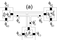
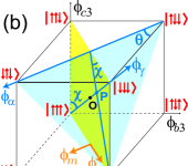
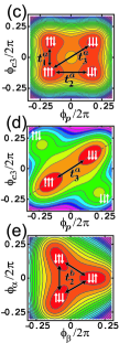
Figure 1: (Color online.) (a) A three flux qubit system. The black squares are the Josephson junctions. The Josephson coupling energy of the Josephson junctions in the qubit and connecting loop are $E_{Ji}$ and $E^{\prime}_{J}$, respectively. $f_{q}$’s are the external fluxes and $\phi$’s are the phase differences across the junctions. (b) The eight states of three qubits are represented in $(\phi_{a3},\phi_{b3},\phi_{c3})$-space at the coresonance point. $(\phi_{\alpha},\phi_{\beta},\phi_{\gamma})$ are the rotated coordinates and O(0,0,0) is the origin of both coordinates. The blue (light gray) triangle intersects vertically the $\phi_{\gamma}$ axis at point P. For $E_{J1}/E_{J}=0.7$, the effective potentials $U_{\rm eff}$ in $(\phi_{p},\phi_{c3})$-plane ( yellow (dark gray) square in (b)) are plotted for (c) $E^{\prime}_{J}=0$ and (d) $E^{\prime}_{J}/E_{J}=0.5$. The dotted line in (d) coincides with $\phi_{\gamma}$ axis in (b). (e) The effective potential $U_{\rm eff}$ in $(\phi_{\alpha},\phi_{\beta})$-plane (blue (light gray) triangle in (b)) for $E^{\prime}_{J}/E_{J}=0.05$ and $E_{J1}/E_{J}=0.75$. Here and after, the superscript $a(b)$ in $t^{a(b)}_{i}$ denotes the tunnelling processes including (excluding) the states, $|\uparrow\uparrow\uparrow\rangle$ or $|\downarrow\downarrow\downarrow\rangle$, and $i=1,2,3$ the single-, two-, and three-qubit tunnelling processes, respectively.

In order to study the GHZ state, $\left|\Psi_{\rm GHZ}\right\rangle=\left(\left|\uparrow\uparrow\uparrow\right\rangle+\left|\downarrow\downarrow\downarrow\right\rangle\right)/\sqrt{2}$, we draw the yellow (dark gray) square introducing the auxiliary coordinates defined by $\phi_{p}\equiv(\phi_{a3}+\phi_{b3})/\sqrt{2}$ and $\phi_{m}\equiv(\phi_{a3}-\phi_{b3})/\sqrt{2}$, while for W state, $\left|\Psi_{\rm W}\right\rangle=\left(\left|\uparrow\downarrow\downarrow\right\rangle+\left|\downarrow\uparrow\downarrow\right\rangle+\left|\downarrow\downarrow\uparrow\right\rangle\right)/\sqrt{3}$, we consider the blue (light gray) triangle. Figures 1(c)-(e) show the effective potential $U_{\rm eff}(\bm{\phi})$ in Eq. (4). When the three qubits are decoupled for $E^{\prime}_{J}=0$ KimTwo ; KimCont , Fig. 1(c) shows that the single-qubit tunneling, $t^{a}_{1}$, is dominant over the three-qubit tunneling, $t^{a}_{3}$. As $E^{\prime}_{J}$ increases, it is shown in Fig. 1(d) that the three-qubit tunneling becomes dominant. Then the GHZ state is expected to be formed at the ground state. The dotted line in Fig. 1(d) coincides with $\phi_{\gamma}$ axis in Fig. 1(b). Along the $\phi_{\gamma}$ axis, the double-well potential is given by $U_{\rm eff}(0,0,\phi_{\gamma},\sqrt{3}\pi)=3E_{J1}\left(1+\cos\frac{2\phi_{\gamma}}{3}\right)+6E_{J}\left(1-\cos\frac{\phi_{\gamma}}{3}\right),$ where the barrier hight is proportional to $E_{J1}$. The WKB approximation allows us to calculate the three-qubit tunneling, $t^{a}_{3}$, through this double-well potential Orlando ; KimOne . Other tunnelings such as single-qubit tunnelings, $t^{a}_{1}$ and $t^{b}_{1}$, and two-qubit tunnelings, $t^{a}_{2}$ and $t^{b}_{2}$, can also be calculated. The tight-binding approximation based on the eight states of three qubits gives the effective Hamiltonian, $H=\sum_{\nu}E_{\nu}|\nu\rangle\langle\nu|-\sum_{\nu,\nu^{\prime}}t_{\nu\nu^{\prime}}|\nu\rangle\langle\nu^{\prime}|,$ where $t_{\nu\nu^{\prime}}=t^{a(b)}_{i}$ and $|\nu\rangle=|s_{a}s_{b}s_{c}\rangle$ with $s_{q}\in\{\uparrow,\downarrow\}$.

Q-measure.$-$ The global entanglement for tripartite systems can be quantified by the Q-measure Meyer . For a normalized arbitrary three-qubit state, $|\Psi\rangle=c_{1}\left|\downarrow\downarrow\downarrow\right\rangle+c_{2}\left|\downarrow\downarrow\uparrow\right\rangle+c_{3}\left|\downarrow\uparrow\downarrow\right\rangle+c_{4}\left|\downarrow\uparrow\uparrow\right\rangle+c_{5}\left|\uparrow\downarrow\downarrow\right\rangle+c_{6}\left|\uparrow\downarrow\uparrow\right\rangle+c_{7}\left|\uparrow\uparrow\downarrow\right\rangle+c_{8}\left|\uparrow\uparrow\uparrow\right\rangle$, the Q-factor is given by

$$Q(|\Psi\rangle)=\frac{4}{3}\sum^{3}_{j=1}D_{j}(|\Psi\rangle),$$ (9)

where $D_{1}(|\Psi\rangle)=|c_{1}c_{6}-c_{2}c_{5}|^{2}+|c_{1}c_{7}-c_{3}c_{5}|^{2}+|c_{1}c_{8}-c_{4}c_{5}|^{2}+|c_{2}c_{7}-c_{3}c_{6}|^{2}+|c_{2}c_{8}-c_{4}c_{6}|^{2}+|c_{3}c_{8}-c_{4}c_{7}|^{2}$ and $D_{2}(|\Psi\rangle)$ and $D_{3}(|\Psi\rangle)$ are obtained by exchanging the indices as $3\leftrightarrow 5,4\leftrightarrow 6$ for $D_{2}$ and $2\leftrightarrow 5,4\leftrightarrow 7$ for $D_{3}$. For the GHZ state, $Q(|\Psi_{\rm GHZ}\rangle)=1$ and for the W state $Q(|\Psi_{\rm W}\rangle)=8/9$.

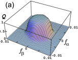
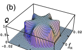
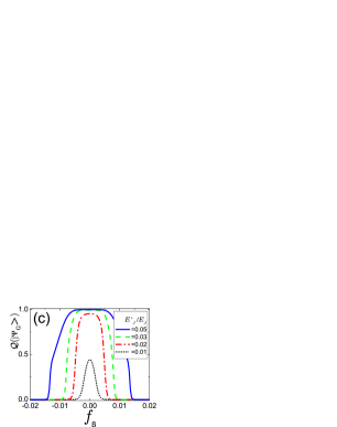
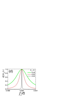
Figure 2: (Color online.) The Q-factors of the ground state in the three qubit system for (a) $E^{\prime}_{J}/E_{J}=0.02$ and for (b) $E^{\prime}_{J}/E_{J}=0.05$. Here, $f_{\gamma}=\sqrt{3}/2$ and $E_{J1}/E_{J}=0.7$. (c) Cut view of Q-factors in (a) and (b) for $f_{\alpha}=0$. (d) For $f_{\alpha}=f_{\beta}=0$ and $E^{\prime}_{J}/E_{J}=0.6$, Q-factors are plotted as a function of $f_{\gamma}$ for several $E_{J1}$.

GHZ state.$-$We plot the Q-factors for the ground state in Figs. 2(a) and (b) as a function of the rotated fluxes $f_{\alpha}\equiv(f_{a}-f_{b})/\sqrt{2},f_{\beta}\equiv(f_{a}+f_{b}-2f_{c})/\sqrt{6},f_{\gamma}\equiv(f_{a}+f_{b}+f_{c})/\sqrt{3}$. Note that the coresonance point $(f_{a},f_{b},f_{c})=(1/2,1/2,1/2)$ is transformed to $(f_{\alpha},f_{\beta},f_{\gamma})=(0,0,\sqrt{3}/2)$. For $E^{\prime}_{J}/E_{J}=0.02$ in Fig. 2 (a), $Q<1$. But, as $E^{\prime}_{J}$ increases, the GHZ state appears around the coresonance point in Fig. 2 (b). Figure 2 (c) is the cut view of Q-factor for various coupling strength. It is found that for the GHZ state, $E^{\prime}_{J}$ should be larger than $0.03E_{J}$. It turns out that the coupling strength from the inductive coupling scheme corresponds to $E^{\prime}_{J}\approx 0.005E_{J}$ KimTwo . This shows that the inductive coupling scheme cannot provide a sufficient coupling for the GHZ state.

To be observed experimentally, the GHZ state should be robust against fluctuations of external flux. Figure 2(b) shows that the GHZ state can be obtained for a broad range of $f_{\alpha}$ and $f_{\beta}$. Thus, let us examine the behavior of Q-factor as a function of $f_{\gamma}$ (Fig. 2(d)). If the peak width is too narrow compared with the fluctuations of external flux, the GHZ state cannot be observed experimentally. Actually, it is found that the three-qubit tunneling $t^{a}_{3}$ plays an important role for wide peak width. If other tunneling processes except $t^{a}_{3}$ are negligible, small flux fluctuations can influence the Q-factor given approximately by $Q(|\Psi\rangle)\approx(t^{a}_{3})^{2}/((\delta E)^{2}+(t^{a}_{3})^{2})$, where $\delta E$ is the energy level change with $E_{\downarrow\downarrow\downarrow}=E_{g}+\delta E$ and $E_{\uparrow\uparrow\uparrow}=E_{g}-\delta E$, $E_{g}$ the ground state energy and $\delta E\propto(f_{\gamma}/\sqrt{3}-0.5)$ KimTwo . Qualitatively, then, $t^{a}_{3}$ corresponds to the peak width of the envelope of Q-factor in Fig. 2(d). Consequently, the stronger $t^{a}_{3}$, the wider the range for the GHZ state.

But the single-qubit tunnelling $t^{a}_{1}$ makes the coupled qubits unentangled. Thus we need to suppress the single-qubit tunnelling, while enhancing the three-qubit tunnelling. In order to do so we need strong coupling as shown in Fig. 1(d), where the single-qubit tunnellings between the ground and excited levels become suppressed. On the other hand the relevant parameter for $t^{a}_{3}$ is the Josephson coupling energy $E_{J1}$. As $E_{J1}$ decreases, the barrier in the double-well potential in Fig. 1(d) becomes lower. It implies that, to get a larger value of $t^{a}_{3}$, $E_{J1}$ should be smaller. But too small $E_{J1}$ makes some excited states, $|s_{a}s_{b}s_{c}\rangle$, unstable. We show the minimum $E_{J1}$’s in Table I for three representative $E^{\prime}_{J}$’s. In fact, we found that for strong coupling case the excited states are stable for smaller $E_{J1}$. For small $E^{\prime}_{J}/E_{J}=0.05$ we obtained $t^{a}_{1}/E_{J}=1.3\times 10^{-3}$ and thus $t^{a}_{3}/t^{a}_{1}\approx 5.4\times 10^{-3}$. But for larger value of $E^{\prime}_{J}/E_{J}=0.6$ we obtained $t^{a}_{3}/t^{a}_{1}\approx 6.4$ with $t^{a}_{1}/E_{J}=8.0\times 10^{-4}$. Hence for strong coupling case we can expect higher Q-factor for the GHZ state.

In Table I the peak widths for both GHZ and W states are calculated at 95% of the maximum value of Q-factor, which are approximately proportional to $t^{a}_{3}$ and $t^{b}_{2}$, respectively. During the Rabi oscillations the fluctuation of flux is estimated to be in the order of $10^{-6}[\Phi_{0}/Hz^{1/2}]$ Bertet and $1/f$ critical current fluctuations of the Josephson junctions is rather weak. In recent experiments for flux qubits, the flux amplitudes are controlled up to the accuracy of $10^{-5}\Phi_{0}$. In this respect, the peak width, $\delta f_{\gamma}\sim 4\times 10^{-4}$, for $E^{\prime}_{J}=0.6E_{J}$ will be sufficient to observe the GHZ state experimentally.

$E^{\prime}_{J}$	$E_{J1}$	$t^{a}_{3}$	peak width	$t^{b}_{2}$	peak width
			GHZ ($\delta f_{\gamma}$)		W ($\delta f_{\alpha}$)
0.05	0.7	7.0 $\times 10^{-6}$	$\sim\!\!5\times 10^{-7}$	6.3 $\times 10^{-4}$	$\sim\!\!10^{-4}$
0.1	0.75	2.6 $\times 10^{-7}$	$\sim\!\!2\times 10^{-8}$	1.0 $\times 10^{-4}$	$\sim\!\!2\times 10^{-5}$
0.6	0.58	5.1 $\times 10^{-3}$	$\sim\!\!4\times 10^{-4}$	0	0

Table 1: Peak widths for Q-factors of GHZ state in Fig. 2(d) and of W state in Fig. 3(d) at 95% of the maximum values. Here the unit of $E^{\prime}_{J}$, $E_{J1}$, and $t$ is $E_{J}$.

W state.$-$ In Fig. 1(b), we present the blue (light gray) triangle whose corners correspond to the three states consisting of the W state, $|\Psi_{\rm W}\rangle=\left(\left|\uparrow\downarrow\downarrow\right\rangle+\left|\downarrow\uparrow\downarrow\right\rangle+\left|\downarrow\downarrow\uparrow\right\rangle\right)/\sqrt{3}$. The blue (light gray) triangle intersects $\phi_{\gamma}$-axis at $\phi_{\gamma}>0$. Actually, there is another intersection plane with $\phi_{\gamma}<0$ for another possible W state. For simplicity, we will focus on the W state on the blue (light gray) triangle plane. The effective potential at the plane of the blue (light gray) triangle for the three states is drawn in Fig. 1(e). Energetically, in our model, the energies of three states are higher than those of the two states consisting of the GHZ state, i.e., the ground state. Then, the W state can be observed in an excited state.

Let us discuss how a W state can be realized in an excited state. At the coresonance point $(f_{\alpha},f_{\beta},f_{\gamma})=(0,0,\sqrt{3}/2)$, the six states except for $\{\left|\downarrow\downarrow\downarrow\right\rangle,\left|\uparrow\uparrow\uparrow\right\rangle\}$ are degenerated in the second excited state. The six states are classified into two classes, $\{\left|\uparrow\uparrow\downarrow\right\rangle,\left|\uparrow\downarrow\uparrow\right\rangle,\left|\downarrow\uparrow\uparrow\right\rangle\}$ with $S_{z}=1/2$ and $\{\left|\uparrow\downarrow\downarrow\right\rangle,\left|\downarrow\uparrow\downarrow\right\rangle,\left|\downarrow\downarrow\uparrow\right\rangle\}$ with $S_{z}=-1/2$. Hence, the two classes of the six states can be separated by applying an additional flux $\Delta f_{\gamma}$. The three states of each class can form a W state. As shown in Fig. 1(e), the two-qubit tunneling amplitude $t^{b}_{2}$ creates the W-state, while the single-qubit tunneling $t^{b}_{1}$ destroys the W-state because it induces a superposition of states of the two classes. If other small tunnelings are negligible, then, the Q-factor is given by $Q(|\Psi\rangle)\simeq 8(1+2.5(t^{b}_{1}/\Delta E)^{2})/9(1+4(t^{b}_{1}/\Delta E)^{2})$. From $Q(|\Psi_{\rm W}\rangle)=8/9$, it turns out that $|\Delta E|\propto|f_{\gamma}/\sqrt{3}-1/2|$ should be much larger than $t^{b}_{1}$. Therefore, a sufficient $\Delta f_{\gamma}$ are needed to generate a W state. Actually, we found that $|\Delta f_{\gamma}|\gtrsim 0.01$ is sufficient to show the generation of a W state (Figs. 3(a) and (b)). In Fig. 3(b), the W state is formed slightly away from the point, $f_{\alpha}=f_{\beta}=0$. For a relatively weak coupling the single-qubit tunneling $t^{b}_{1}$ as well as $t^{b}_{2}$ becomes larger. Thus, an additional small flux $f_{\beta}\approx 0.0004$ will break the symmetry so that the state $|\Psi\rangle$ closer to the W state would be formed. In Fig. 3(c) we can see the W state around $f_{\alpha}=0$.

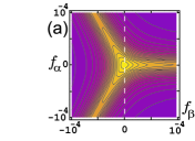
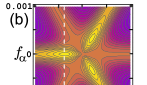
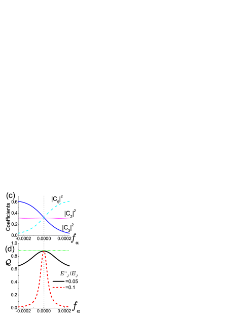
Figure 3: (Color online.) The Q-factors of the second excited state with $f_{\gamma}=\sqrt{3}/2-0.01$ for (a) $E^{\prime}_{J}/E_{J}=0.1$ and $E_{J1}/E_{J}=0.75$ and (b) $E^{\prime}_{J}/E_{J}=0.05$ and $E_{J1}/E_{J}=0.7$. Note the different scales and positions of maximum Q-factor in both figures. Here the yellow (light gray) regions denote high Q-factors. (c) The coefficients of the eigenstate used in (b) are plotted along the dotted line with $f_{\beta}=-0.0004$, which shows that W state is formed around $f_{\alpha}=0$. (d) Cut view of Q-factors along dotted lines in (a) and (b). The green dotted line indicates $Q=8/9$ for W state. The peak width for $E^{\prime}_{J}/E_{J}=0.05$ is much wider than that for $E^{\prime}_{J}/E_{J}=0.1$.

On the contrary to the GHZ state where the range of $f_{\gamma}$ is critical for experimental observation, for W state the range in $(f_{\alpha},f_{\beta})$-plane is important as shown in Figs. 3(a) and (b). Fig. 3(d) shows the Q-factor for W-states whose peak widths depend on the value of the two-qubit tunneling amplitude $t^{b}_{2}$ (Table I). As $E^{\prime}_{J}$ decreases, $t^{b}_{2}$ becomes larger. However, if the coupling strength becomes too weak, the two classes with $S_{z}=\pm 1/2$ will become overlapped with each other through the single qubit tunnelling $t^{b}_{1}$ so that the W state may readily be broken. Hence, as a consequence of compromise, the W state emerges for an intermediate coupling strength, $E^{\prime}_{J}=0.05E_{J}$, with rather broader peak width as shown in Table I.

Discussions and summary.$-$The quantification of entanglement can be done by using the state tomography measurement Steffen ; Liu . Recently for capacitively coupled phase qubits the tomography measurement has been done Steffen , where they simultaneously measure the state of coupled qubits. For present coupling we expect that the similar tomography measurement can also be performed.

The tripartite entanglement with superconducting qubits has not yet been achieved so far. For the bipartite entanglement capacitively coupled phase qubits showed high fidelity in a recent experiment Steffen , while for charge qubits only partial entanglement was observed. The interaction between phase qubits are XY-type interaction which describes simultaneous two-qubit flipping processes. The two- or multiple-qubit tunnelling processes are essential for entanglement of qubits KimCho . However, for charge qubits, the interaction are mainly Ising-type. We believe that this is the reason for weak entanglement in experiments with charge qubits. For three coupled phase qubits the lowest energy state is $|000\rangle$ state while the highest is $|111\rangle$ state. Hence the superposition between these two states will be negligibly weak, thus the GHZ state cannot be formed. But, since the other states, for example $|100\rangle,|010\rangle,|001\rangle$ states, are energetically degenerated, the W state could be obtained.

In summary, we investigate a three superconducting flux qubit system. The GHZ and W states can be realizable in the eigenstates of the macroscopic quantum system. We show that while the GHZ state needs strong coupling strength, the W state can be formed at an optimized coupling strength. Moreover, to keep the tripartite entangled states robust against external flux fluctuations for feasible experimental realizations, the three coupled qubit system can provide relatively large three-qubit and two-qubit tunneling amplitudes for GHZ and W states, respectively.

SYC acknowledges the support from the Australian Research Council.

References

(1)
D. M. Greenberger, M. A. Horne, and A. Zeilinger, in
Bell s Theorem, Quantum Theory, and Conceptions of the Universe, edited by
M. Kafatos (Kluwer Academics, Dordrecht, 1989).
(2)
A. Zeilinger, M. A. Horne, and D. M. Greenberger, in
Proceedings of the Workshop on Squeezed States and Quantum
Uncertainty, edited by D. Han, Y. S. Kim, and W.W. Zachary
(NASA, Washington DC, 1992).
(3)
W. Dür, G. Vidal, and J. I. Cirac, Phys. Rev. A 62, 062314
(2000).
(4)
A. Rauschenbeutel, G. Nogues, S. Osnaghi, P. Bertet, M. Brune, J.-M. Raimond, and S. Haroche,
Science 288, 2024 (2000).
(5) D. Bouwmeester, J.-W. Pan, M. Daniell, H. Weinfurter, and A. Zeilinger,
Phys. Rev. Lett. 82, 1345 (1999);
J.-W. Pan, D. Bouwmeester, M. Daniell, H. Weinfurter, and A. Zeilinger,
Nature 403, 515 (2000);
J.-W. Pan, M. Daniell, S. Gasparoni, G. Weihs, and A. Zeilinger, Phys. Rev. Lett. 86, 4435 (2001);
M. Eibl, N. Kiesel, M. Bourennane, C. Kurtsiefer, and H. Weinfurter, Phys. Rev. Lett. 92, 077901 (2004).
(6)
C. F. Roos, M. Riebe, H. Haffner, W. Hansel, J. Benhelm, G. P. T. Lancaster,
C. Becher, F. Schmidt-Kaler, and R. Blatt, Science 304, 1478 (2004);
D. Leibfie, M. D. Barrett, T. Schaetz, J. Britton, J. Chiaverini, W. M. Itano,
J. D. Jost, C. Langer, and D. J. Wineland,
Science 304, 1476 (2004).
(7)
Yu. A. Pashkin, T. Yamamoto, O. Astafiev, Y. Nakamura, D. V. Averin, and J. S. Tsai,
Nature 421, 823 (2003); T. Yamamoto, Yu. A. Pashkin, O. Astafiev, Y. Nakamura,
and J. S. Tsai, ibid.425, 941 (2003).
(8)
A. J. Berkley, H. Xu, R. C. Ramos, M. A. Gubrud, F. W. Strauch, P. R. Johnson,
J. R. Anderson, A. J. Dragt, C. J. Lobb, and F. C. Wellstood,
Science 300, 1548 (2003).
(9) M. Steffen, M. Ansmann, R. C. Bialczak, N. Katz, E. Lucero,
R. McDermott, M. Neeley, E. M. Weig, A. N. Cleland, and J. M. Martinis,
Science 313, 1423 (2006);
R. McDermott, R. W. Simmonds, M. Steffen, K. B. Cooper, K. Cicak, K. D. Osborn,
S. Oh, D. P. Pappas, and John M. Martinis, ibid.307, 1299 (2005).
(10)
A. Izmalkov, M. Grajcar, E. Iĺichev, Th. Wagner, H.-G. Meyer,
A.Yu. Smirnov, M. H. S. Amin, Alec Maassen van den Brink, and A.M. Zagoskin,
Phys. Rev. Lett. 93, 037003 (2004);
A. O. Niskanen, K. Harrabi, F. Yoshihara, Y. Nakamura, S. Lloyd, and J. S. Tsai,
Science 316, 723 (2007).
(11) J. H. Plantenberg, P. C. de Groot, C. J. P. M. Harmans, and J. E. Mooij,
Nature 447, 836 (2007).
(12) M. D. Kim and S. Y. Cho, Phys. Rev. B 75 134514 (2007).
(13) L. F. Wei, Y.-x. Liu, and F. Nori, Phys. Rev. Lett. 96, 246803 (2006).
(14) J. B. Majer, F. G. Paauw, A. C. J. ter Haar, C. J. P. M. Harmans, and J. E. Mooij,
Phys. Rev. Lett. 94, 090501 (2005).
(15) M. D. Kim and J. Hong, Phys. Rev. B 70, 184525 (2004).
(16) M. Grajcar,Y.-X. Liu, F. Nori, and A. M. Zagoskin,
Phys. Rev. B 74, 172505 (2006).
(17) M. D. Kim, Phys. Rev. B 74, 184501 (2006).
(18) S. H. W. van der Ploeg,
A. Izmalkov,
Alec Maassen van den Brink, U. Hübner, M. Grajcar, E. Iĺichev,
H.-G. Meyer, and A.M. Zagoskin,
Phys. Rev. Lett. 98, 057004 (2007).
(19) S. Y. Cho and M. D. Kim, cond-mat/0703505.
(20) J. E. Mooij, T. P. Orlando, L. Levitov, Lin Tian, Caspar H. van der Wal, and Seth Lloyd,
Science 285, 1036 (1999);
Caspar H. van der Wal, A. C. J. ter Haar, F. K. Wilhelm, R. N. Schouten, C. J. P. M. Harmans,
T. P. Orlando, Seth Lloyd, and J. E. Mooij,
ibid.290, 773 (2000); I. Chiorescu, Y. Nakamura, C. J. P. M. Harmans,
and J. E. Mooij, ibid.299, 1869 (2003);
I. Chiorescu, P. Bertet, K. Semba, Y. Nakamura, C. J. P. M. Harmans, and J. E. Mooij,
Nature 431, 159 (2004);
T. Hime, P. A. Reichardt, B. L. T. Plourde, T. L. Robertson, C.-E. Wu,
A. V. Ustinov, and J. Clarke, Science 314, 1427 (2006).
(21) T. P. Orlando, J. E. Mooij, Lin Tian, Caspar H. van der Wal, L. S. Levitov, Seth Lloyd, and J. J. Mazo,
Phys. Rev. B 60, 15398 (1999).
(22) M. D. Kim, D. Shin, and J. Hong,
Phys. Rev. B 68, 134513 (2003).
(23) D. A. Meyer and N. R. Wallach, J. Math. Phys. 43, 4273 (2002).
(24)
F. Yoshihara, K. Harrabi, A. O. Niskanen, Y. Nakamura, and J. S. Tsai,
Phys. Rev. Lett. 97, 167001 (2006);
P. Bertet, I. Chiorescu, G. Burkard, K. Semba, C. J. P. M. Harmans, D. P. DiVincenzo,
and J. E. Mooij, ibid.95, 257002 (2005).
(25) Y.-x. Liu, L. F. Wei, and F. Nori, Phys. Rev. B 72, 014547 (2005).