Average Stopping Set Weight Distribution of Redundant Random Matrix Ensembles

Abstract

In this paper, redundant random matrix ensembles (abbreviated as redundant random ensembles) are defined and their stopping set (SS) weight distributions are analyzed. A redundant random ensemble consists of a set of binary matrices with linearly dependent rows. These linearly dependent rows (redundant rows) significantly reduce the number of stopping sets of small size. An upper and lower bound on the average SS weight distribution of the redundant random ensembles are shown. From these bounds, the trade-off between the number of redundant rows (corresponding to decoding complexity of BP on BEC) and the critical exponent of the asymptotic growth rate of SS weight distribution (corresponding to decoding performance) can be derived. It is shown that, in some cases, a dense matrix with linearly dependent rows yields asymptotically (i.e., in the regime of small erasure probability) better performance than regular LDPC matrices with comparable parameters.

Keywords

LDPC codes, Stopping set, Weight distribution, Ensemble

I Introduction

On binary erasure channel (BEC), the decoding performance of belief propagation (BP)-based iterative decoder of low-density parity-check(LDPC) codes is dominated by combinatorial structures in a Tanner graph, which are called stopping sets (SS)[1]. Di et al.[1] introduced the idea of stopping sets and presented a recursive method to evaluate the average block and bit error probabilities of LDPC codes[8] of finite length on BEC[1]. Orlitsky et al. [2] found the asymptotic behavior of the SS weight distributions of bipartite graph ensembles and extended the results of Di et al. to the irregular code case.

For a given binary linear code $C$, it is hoped to find the best representation of $C$ (i.e., a parity check matrix) which yields the smallest block (or bit) error probability when it is decoded with iterative decoding on BEC. A parity check matrix which defines $C$ can be a redundant parity check matrix, which is not a full-rank matrix: that is, it can contain some linearly dependent rows. For example, some finite geometry LDPC codes require a redundant parity check matrix to achieve good decoding performance with BP. Recent works of Schwartz and Vardy[3], Abdel-Ghaffar and Weber[4], Hollmann and Tolhuizen[5] indicate that the stopping set weight distribution of a given matrix can be improved by appending linearly dependent rows to the original matrix.

Recent developments described in studies of the average weight distributions of LDPC codes, such as Litsyn and Shevelev[9][10], Burshtein and Miller[11] Richardson and Urbanke[6], imply that ensemble analysis is a powerful method for investigating typical properties of codes and matrices, properties are not easy to obtain from an instance. Furthermore, from the asymptotic behavior of typical properties such as these, we often can predict a threshold phenomenon.

The average stopping set weight distributions presented in [1] and [2] are a useful decoding performance measure (for BP on BEC) of a given ensemble of parity check matrices. The distribution can be used for optimizing an ensemble suitable for BEC. BEC is not only of practical interest, but also can be considered as a good starting point for theoretical studies of performance analysis of BP for more general channels, such as binary input symmetric output channels[6].

In this paper, redundant random matrix ensembles (abbreviated as redundant random ensembles) are defined and their SS weight distributions are analyzed. The redundant random ensemble consists of a set of binary matrices with linearly dependent rows. These linearly dependent rows (redundant rows) significantly reduce the number of stopping sets of small size. An upper bound and a lower bound on the average SS weight distribution of redundant random ensemble will be shown. From these bounds, the trade-off between the number of redundant rows (corresponding to decoding complexity of BP) and the critical exponent of the asymptotic growth rate of SS weight distribution (corresponding to decoding performance) can be derived.

II Average SS weight distribution

In this section, some notation and definitions required in the paper are introduced. Furthermore, some known results on average SS weight distributions are briefly reviewed.

II-A Stopping set and SS weight distribution

Let $F_{2}$ be the binary Galois field with elements $\{0,1\}$. The operator $\circ$ denotes the integer ring inner product defined by $\mbox{\boldmath$h$}\circ\mbox{\boldmath$x$}\stackrel{{\scriptstyle\triangle}}{{=}}h_{1}x_{1}+h_{2}x_{2}+\cdots+h_{n}x_{n}$ for $\mbox{\boldmath$h$}\stackrel{{\scriptstyle\triangle}}{{=}}(h_{1},h_{2},\ldots,h_{N})\in F_{2}^{n}$ and $\mbox{\boldmath$x$}\stackrel{{\scriptstyle\triangle}}{{=}}(x_{1},x_{2},\ldots,x_{n})\in F_{2}^{n}$ $(n\geq 1)$. The additions in the above definition of $\circ$ is the addition of the integer ring (i.e., $1+1=2$). In this paper, the addition of $F_{2}$ is denoted by $\oplus$ (i.e., $1\oplus 1=0$).

For a given $\mbox{\boldmath$x$}\in F_{2}^{n}$ and an $m\times n$ binary matrix $H$ $(m,n\geq 1)$, the SS indicator $q_{H}(\mbox{\boldmath$x$})$ is defined by

$$q_{H}(\mbox{\boldmath$x$})\stackrel{{\scriptstyle\triangle}}{{=}}\#\{i\in[1,m]:\mbox{\boldmath$h$}_{i}\circ\mbox{\boldmath$x$}=1\},$$ (1)

where $\mbox{\boldmath$h$}_{i}$ denotes the $i$-th row vector of $H$, and we denote the cardinality of a given finite set $X$ by $\#X$. The notation $[a,b]$ means the set of consecutive integers from $a$ to $b$. The stopping set is defined as follows:

Definition 1 (Stopping set)

If $q_{H}(\mbox{\boldmath$x$})=0$ then $\mbox{\boldmath$x$}\in F_{2}^{n}$ is called a SS vector of $H$. The support set of $x$,

$$S_{\mbox{\boldmath$x$}}\stackrel{{\scriptstyle\triangle}}{{=}}\{i\in[1,n]:x_{i}=1\},$$ (2)

is called a stopping set of $H$. ∎

Note that if there exists a row vector $\mbox{\boldmath$h$}_{i}(i\in[1,m])$ satisfying $\mbox{\boldmath$h$}_{i}\circ\mbox{\boldmath$x$}=1$ then $x$ is not an SS vector. Let $\mbox{\boldmath$y$}\stackrel{{\scriptstyle\triangle}}{{=}}(y_{1},y_{2},\ldots,y_{n})\in\{0,1,e\}^{n}$ be a received word through a BEC, where $e$ denotes the erasure symbol. It is known that BP fails to decode $y$ if and only if the erasure support set $E_{\mbox{\boldmath$y$}}\stackrel{{\scriptstyle\triangle}}{{=}}\{i\in[1,n]:y_{i}=e\}$ contains a non-empty stopping set of $H$. This property justifies the study of SSs in order to reveal the BP decoding performance for BEC.

The next definition provides the definition of the SS weight distribution and the stopping distance:

Definition 2 (SS weight distribution and stopping distance)

For a given $m\times n(m,n\geq 1)$ matrix $H$, the SS weight distribution $\{S_{w}(H)\}_{w=0}^{n}$ is defined by

$$S_{w}(H)\stackrel{{\scriptstyle\triangle}}{{=}}\sum_{\mbox{\boldmath$x$}\in Z^{(n,w)}}I[q_{H}(\mbox{\boldmath$x$})=0]$$ (3)

for $0\leq w\leq n$, where $Z^{(n,w)}$ is the set of constant weight binary vectors of length $n$ whose Hamming weights are $w$. The notation $I[condition]$ is the indicator function such that $I[condition]=1$ if $condition$ is true; otherwise, it gives 0. The stopping distance of $H$ is defined by

$$\Delta(H)\stackrel{{\scriptstyle\triangle}}{{=}}\min\{w\in[1,n]:S_{w}(H)\neq 0\}.$$ (4)

∎

Example 1

Let

$$H=\left(\begin{array}[]{ccc}1&0&1\\ 1&1&1\\ \end{array}\right).$$ (5)

In this case, $W\stackrel{{\scriptstyle\triangle}}{{=}}\{\emptyset,\{1,3\},\{1,2,3\}\}$ is the set of stopping sets of $H$ and $2^{[1,n]}\backslash W$ is the set of non-stopping sets of $H$. The SS weight distribution is given by $\{S_{w}(H)\}_{w=0}^{3}=\{1,0,1,1\}$ and the stopping distance is $\Delta(H)=2$. ∎

II-B Average SS weight distribution

Suppose that ${\cal G}$ is a set of binary $m\times n$ matrices$(m,n\geq 1)$. Note that we allow the possibility that ${\cal G}$ may contain some matrices with the same configuration. Such matrices should be distinguished as distinct matrices. We assign the same probability, $1/\#{\cal G}$, to each matrix in ${\cal G}$. Let $f(H)$ be a real-valued function which depends on $H\in{\cal G}$. The expectation of $f(H)$ with respect to the ensemble ${\cal G}$ is defined by

$$E_{{\cal G}}[f(H)]\stackrel{{\scriptstyle\triangle}}{{=}}\sum_{H\in{\cal G}}P(H)f(H)=\frac{1}{\#{\cal G}}\sum_{H\in{\cal G}}f(H).$$ (6)

The average SS weight distribution is defined as follows:

Definition 3 (Average SS weight distribution)

The average SS weight distribution of a given ensemble ${\cal G}$ is defined by

$$S_{w}^{{\cal G}}\stackrel{{\scriptstyle\triangle}}{{=}}E_{\cal G}[S_{w}(H)]$$ (7)

for $0\leq w\leq n$. ∎

One of the most important properties of an ensemble is its symmetry. Although several types of symmetry are shown to be useful in [12], the following simple definition is sufficient for the purposes of this paper.

Definition 4 (Symmetry of an ensemble)

If the equality

$$\#\{H\in{\cal G}:q_{H}(\mbox{\boldmath$x$}_{1})=0\}=\#\{H\in{\cal G}:q_{H}(\mbox{\boldmath$x$}_{2})=0\}$$ (8)

holds for any $\mbox{\boldmath$x$}_{1},\mbox{\boldmath$x$}_{2}\in Z^{(n,w)}$ and any $w\in[0,n]$, then the ensemble ${\cal G}$ is called symmetric. ∎

There is a simple expression of the average SS weight distribution for a symmetric ensemble. . The next lemma shows that the evaluation of the average SS weight distribution is equivalent to a counting problem of matrices satisfying a certain condition.

Lemma 1

If ${\cal G}$ is symmetric, then

$$S_{w}^{{\cal G}}=\frac{{n\choose w}}{\#{\cal G}}\#\{H\in{\cal G}:q_{H}(\mbox{\boldmath$x$}_{w})=0\}$$ (9)

holds for $w\in[0,n]$. The vector $\mbox{\boldmath$x$}_{w}\in Z^{(n,w)}$ is the binary vector whose first $w$-elements are one, with all other elements zero.
(Proof) The average SS weight distribution of ${\cal G}$ can be transformed into the following form,

$$S_{w}^{{\cal G}} = E_{\cal G}[S_{w}(H)]$$ (10)

$$= \sum_{H\in{\cal G}}P(H)\sum_{\mbox{\boldmath$x$}\in Z^{(n,w)}}I[q_{H}(\mbox{\boldmath$x$})=0]$$

$$= \sum_{\mbox{\boldmath$x$}\in Z^{(n,w)}}\sum_{H\in{\cal G}}P(H)I[q_{H}(\mbox{\boldmath$x$})=0]$$

$$= \frac{1}{\#{\cal G}}\sum_{\mbox{\boldmath$x$}\in Z^{(n,w)}}\#\{H\in{\cal G}:q_{H}(\mbox{\boldmath$x$})=0\}$$

$$= \frac{{n\choose w}}{\#{\cal G}}\#\{H\in{\cal G}:q_{H}(\mbox{\boldmath$x$}_{w})=0\}.$$ (11)

The last equation follows from the assumption; namely $\#\{H\in{\cal G}:q_{H}(\mbox{\boldmath$x$})=0\}$ takes the same value for any $\mbox{\boldmath$x$}\in Z^{(n,w)}$. ∎

II-C Average SS weight distributions of known ensembles

In this subsection, the average SS weight distribution of three well-known ensembles: the random ensemble, the constant row weight ensemble and the bipartite ensemble, will be shown.

II-C1 Random ensemble

The random ensemble ${\cal R}_{m,n}$ is the set of all binary $m\times n$ matrices$(m,n\geq 1)$. Thus, the size of ${\cal R}_{m,n}$ is equal to $2^{mn}$. The following lemma gives the average SS distribution of the random ensemble. The key of the proof is to count $\#\{H\in{\cal R}_{m,n}:q_{H}(\mbox{\boldmath$x$}_{w})=0\}$.

Lemma 2

The average SS distribution of the random ensemble ${\cal R}_{m,n}$ is given by

$$S_{w}^{{\cal R}_{m,n}}={n\choose w}(1-w2^{-w})^{m}$$ (12)

for $0\leq w\leq n$.
(Proof) From the definition of the ensemble, it is evident that the following equality holds,

$$\#\{H\in{\cal R}_{m,n}:q_{H}(\mbox{\boldmath$x$}_{w})=0\}=(\#\{\mbox{\boldmath$h$}\in F_{2}^{n}:\mbox{\boldmath$h$}\circ\mbox{\boldmath$x$}_{w}\neq 1\})^{m}.$$ (13)

It is easy to show that the equality

$$\#\{\mbox{\boldmath$h$}\in F_{2}^{n}:\mbox{\boldmath$h$}\circ\mbox{\boldmath$x$}_{w}\neq 1\}=(2^{w}-w)2^{n-w}$$ (14)

holds, since

$$\#\{\mbox{\boldmath$h$}\in F_{2}^{n}:\mbox{\boldmath$h$}\circ\mbox{\boldmath$x$}_{w}=1\}=w2^{n-w}.$$ (15)

Combining the above results, we get

$$S_{w}^{{\cal R}_{m,n}} = E_{{\cal R}_{m,n}}[S_{w}(H)]$$ (16)

$$= \frac{1}{\#{\cal R}_{m,n}}{n\choose w}\#\{H\in{\cal R}_{m,n}:q_{H}(\mbox{\boldmath$x$}_{w})=0\}$$

$$= \frac{1}{2^{mn}}{n\choose w}(2^{n}-w2^{n-w})^{m}$$

$$= {n\choose w}(1-w2^{-w})^{m}.$$

Note that in deriving the second equality from the first equality, the symmetric property of the random ensemble and Lemma 1 was used. ∎

The asymptotic growth rate of the average SS distribution (for simplicity, abbreviated as the asymptotic growth rate) of the random ensemble is defined by

$$\lambda_{\ell}\stackrel{{\scriptstyle\triangle}}{{=}}\lim_{n\rightarrow\infty}\frac{1}{n}\log_{2}S_{\ell n}^{{\cal R}_{(1-R)n,n}},$$ (17)

where $R(0<R<1)$ is called design rate and $\ell(0\leq\ell\leq 1)$ is the normalized weight. The asymptotic growth rate reflects the asymptotic (in the limit as $n$ goes to infinity) behavior of the average SS weight distribution for fixed design rate and normalized weight. The next lemma gives the asymptotic growth rate of random ensembles.

Lemma 3

The asymptotic growth rate of the random ensemble is given by

$$\lambda_{\ell}=H(\ell),\quad 0\leq\ell\leq 1,$$ (18)

where $H(x)$ is the binary entropy function defined by

$$H(x)=-x\log_{2}x-(1-x)\log_{2}(1-x).$$ (19)

(Proof) Substituting the average SS weight distribution (12) into expression (17), we have

$$\lambda_{\ell} = \lim_{n\rightarrow\infty}\frac{1}{n}\log_{2}S_{\ell n}^{{\cal R}_{(1-R)n,n}}$$ (20)

$$= \lim_{n\rightarrow\infty}\frac{1}{n}\log_{2}{n\choose\ell n}(1-\ell n2^{-\ell n})^{(1-R)n}$$

$$= \lim_{n\rightarrow\infty}\frac{1}{n}\log_{2}{n\choose\ell n}$$

$$+ \lim_{n\rightarrow\infty}\frac{1}{n}\log_{2}(1-\ell n2^{-\ell n})^{(1-R)n}$$

$$= H(\ell)+(1-R)\lim_{n\rightarrow\infty}\log_{2}(1-\ell n2^{-\ell n})$$

$$= H(\ell).$$

Note that in deriving the fourth equality from the third equality, the following equality

$$\frac{1}{n}\log_{2}{n\choose\ell n}=H(\ell)+o(1),$$ (21)

was used, where $o(1)$ denotes terms which converge to $0$ in the limit as $n\rightarrow\infty$. ∎

II-C2 Constant row weight ensemble

The constant row weight ensemble ${\cal C}_{m,n,r}$ consists of all the binary $m\times n$ matrices whose rows have exactly weight $r$ $(m,n\geq 1,r\geq 1)$. The size of the ensemble is, thus,

$$\#{\cal C}_{m,n,r}={n\choose r}^{m}.$$

The average weight distribution of this ensemble was shown in [9].

The following lemma shows the average SS distribution of ${\cal C}_{m,n,r}$. The proof is similar to that of Lemma 2.

Lemma 4

The average SS distribution of the constant row weight ensemble ${\cal C}_{m,n,r}$ is given by

$$S_{w}^{{\cal C}_{m,n,r}}={n\choose w}\left(1-w\frac{{n-w\choose r-1}}{{n\choose r}}\right)^{m},$$ (22)

for $0\leq w\leq n$.
(Proof) Combining

$$\#\{H\in{\cal C}_{m,n,r}:q_{H}(\mbox{\boldmath$x$}_{w})=0\}\hskip 85.35826pt$$

$$=(\#\{\mbox{\boldmath$h$}\in Z^{(n,r)}:\mbox{\boldmath$h$}\circ\mbox{\boldmath$x$}_{w}\neq 1\})^{m}$$ (23)

and

$$\#\{\mbox{\boldmath$h$}\in Z^{(n,r)}:\mbox{\boldmath$h$}\circ\mbox{\boldmath$x$}_{w}\neq 1\}={n\choose r}-w{n-w\choose r-1},$$ (24)

we have

$$\#\{H\in{\cal C}_{m,n,r}:q_{H}(\mbox{\boldmath$x$}_{w})=0\}=\left({n\choose r}-w{n-w\choose r-1}\right)^{m}.$$ (25)

The average SS weight distribution is thus given by

$$S_{w}^{{\cal C}_{m,n,r}} = \frac{1}{\#{\cal C}_{m,n,r}}\sum_{\mbox{\boldmath$x$}\in Z^{(n,w)}}\#\{H\in G:q_{H}(\mbox{\boldmath$x$})=0\}$$ (26)

$$= \frac{1}{{n\choose r}^{m}}{n\choose w}\left({n\choose r}-w{n-w\choose r-1}\right)^{m}$$

$$= {n\choose w}\left(1-w\frac{{n-w\choose r-1}}{{n\choose r}}\right)^{m}.$$

In the above, the symmetric property of the ensemble is used in deriving the second equality from the first. ∎

The asymptotic growth rate of the constant row weight ensemble is defined by

$$\xi_{\ell}(R,r)\stackrel{{\scriptstyle\triangle}}{{=}}\lim_{n\rightarrow\infty}\frac{1}{n}\log_{2}S_{\ell n}^{{\cal C}_{(1-R)n,n,r}},$$ (27)

for $0<R<1$ and $0\leq\ell\leq 1$. The next lemma gives the explicit form of the average growth rate:

Lemma 5

The asymptotic SS weight distribution of the constant row weight ensembles is given by

$$\xi_{\ell}(R,r)=H(\ell)-(1-R)\log_{2}\left(\frac{1}{1-r\ell(1-\ell)^{r-1}}\right)$$ (28)

for $0<R<1$ and $0\leq\ell\leq 1$.
(Proof) By using the lower and upper bounds on binomial coefficients given by

$$\frac{n^{k}}{k!}\exp\left(-\frac{k^{2}}{n}\right)\leq{n\choose k}\leq\frac{n^{k}}{k!},$$ (29)

we obtain

$$\ell n\frac{{n-\ell n\choose r-1}}{{n\choose r}} \geq \frac{\ell nr(n-\ell n)^{r-1}}{n^{r}}\exp\left(-\frac{(r-1)^{2}}{n-\ell n}\right)$$

$$= r\ell(1-\ell)^{r-1}\exp\left(-\frac{(r-1)^{2}}{n-\ell n}\right)$$

and

$$\ell n\frac{{n-\ell n\choose r-1}}{{n\choose r}} \leq \frac{\ell nr(n-\ell n)^{r-1}}{n^{r}}\exp\left(\frac{r^{2}}{n}\right)$$ (31)

$$= r\ell(1-\ell)^{r-1}\exp\left(\frac{r^{2}}{n}\right).$$

These bounds imply that

$$\ell n\frac{{n-\ell n\choose r-1}}{{n\choose r}}=r\ell(1-\ell)^{r-1}+o(1)$$ (32)

since $r$ is constant (i.e. not a function of $n$). Using this equation, we obtain immediately the asymptotic SS weight distribution,

$$\xi_{\ell}(R,r) = \lim_{n\rightarrow\infty}\frac{1}{n}\log_{2}S_{\ell n}^{{\cal C}_{(1-R)n,n,r}}$$ (33)

$$= \lim_{n\rightarrow\infty}\frac{1}{n}\log_{2}{n\choose\ell n}\left(1-\ell n\frac{{n-\ell n\choose r-1}}{{n\choose r}}\right)^{(1-R)n}$$

$$= H(\ell)+(1-R)\lim_{n\rightarrow\infty}\log_{2}\left(1-\ell n\frac{{n-\ell n\choose r-1}}{{n\choose r}}\right)$$

$$= H(\ell)+(1-R)\log_{2}(1-r\ell(1-\ell)^{r-1}).$$

∎

II-C3 Bipartite ensemble

The bipartite graph ensemble (abbreviated as a bipartite ensemble) ${\cal B}_{n,c,d}$ is the ensemble of regular bipartite graphs of variable node degree $c$ and check node degree $d$. The following lemma is due to Orlitsky et al[2].

Lemma 6 (Orlitsky et al)

The average SS weight distribution of ${\cal B}_{n,c,d}$ is given by

$$S_{w}^{{\cal B}_{n,c,d}}=\frac{\mbox{coef}\left[((1+x)^{d}-dx)^{\frac{c}{d}n},x^{wc}\right]}{{nc\choose wc}}{n\choose w},$$ (34)

where $\mbox{coef}[f(x),x^{i}]$ denotes the coefficient of a polynomial $f(x)$ corresponding to the term $x^{i}$. ∎

The asymptotic growth rate of $(c,d)$-bipartite ensemble is defined by

$$\gamma_{\ell}(c,d)\stackrel{{\scriptstyle\triangle}}{{=}}\lim_{n\rightarrow\infty}\frac{1}{n}\log_{2}S_{\ell n}^{{\cal B}_{n,c,d}}$$ (35)

for $0\leq\ell\leq 1$. It is shown in [2] that the asymptotic growth rate $\gamma_{\ell}(c,d)$ has the form

$$\gamma_{\ell}(c,d)=\frac{c}{d}\log_{e}\left(\frac{(1+x_{0})^{d}-dx_{0}}{x_{0}^{\ell d}}\right)-(c-1)H_{e}(\ell),$$ (36)

where $x_{0}$ is the only positive solution of

$$\frac{x((1+x)^{d-1}-1)}{(1+x)^{d}-dx}=\ell$$ (37)

and $H_{e}(x)$ is the entropy function with base $e$ defined by

$$H_{e}(x)\stackrel{{\scriptstyle\triangle}}{{=}}-x\log_{e}(x)-(1-x)\log_{e}(1-x).$$ (38)

III Average SS weight distributions of redundant random ensemble

In this section, we discuss the average SS weight distributions of extended ensembles obtained from the random ensemble.

III-A Redundant extension

Before commencing a discussion of redundant extensions, it is perhaps worthwhile to consider how some stopping sets can be eliminated by extending a matrix.

Example 2

Consider the matrix

$$H\stackrel{{\scriptstyle\triangle}}{{=}}\left(\begin{array}[]{cccc}0&1&1&1\\ 0&1&1&0\\ 1&0&1&1\\ \end{array}\right).$$ (39)

It is easy to see that $\{2,3,4\}$ is a stopping set (the sub-matrix composed of the second, third and fourth columns has no row of weight 1). Appending (0 0 0 1) (obtained by adding the first and second rows of $H$) to $H$ as a row vector, we have a modified matrix $H^{\prime}$,

$$H^{\prime}\stackrel{{\scriptstyle\triangle}}{{=}}\left(\begin{array}[]{cccc}0&1&1&1\\ 0&1&1&0\\ 1&0&1&1\\ \hline\cr 0&0&0&1\\ \end{array}\right).$$ (40)

We can observe that the weight of the last row of the sub-matrix corresponding to the second, third and fourth columns is 1. This implies that $\{2,3,4\}$ is no longer a stopping set of $H^{\prime}$. Note also that the row spaces spanned by $H$ and $H^{\prime}$ are exactly the same. ∎

The previous example demonstrates the possibility that the SS weight distribution could be improved by adding linearly dependent rows (called redundant rows) to a given matrix.

Let $H$ be a binary $m\times n$ $(1\leq m<n)$ matrix,

$$H\stackrel{{\scriptstyle\triangle}}{{=}}\left(\begin{array}[]{c}\mbox{\boldmath$h$}_{1}\\ \mbox{\boldmath$h$}_{2}\\ \vdots\\ \mbox{\boldmath$h$}_{m}\\ \end{array}\right).$$ (41)

Let $L$ be a positive integer which is a divisor of $m$. For $1\leq i\leq 2^{L}-1$, $0\leq\ell\leq m/L-1$, we define $\mbox{\boldmath$a$}_{i}^{(\ell)}$ by

$$\mbox{\boldmath$a$}_{i}^{(\ell)}\stackrel{{\scriptstyle\triangle}}{{=}}(b_{1}(i),b_{2}(i),\ldots,b_{L}(i))\left(\begin{array}[]{c}\mbox{\boldmath$h$}_{L\ell+1}\\ \mbox{\boldmath$h$}_{L\ell+2}\\ \vdots\\ \mbox{\boldmath$h$}_{L\ell+L}\\ \end{array}\right),$$ (42)

where $b_{j}(i)$ is the $j$-th bit of binary representation of $i$, namely, $i=\sum_{j=1}^{L}2^{j}b_{j}(i).$ In other words, $\mbox{\boldmath$a$}_{i}^{(\ell)}$ is a linear combination of $\mbox{\boldmath$h$}_{L\ell+k}(1\leq k\leq L)$.

The redundant extension of a given matrix is defined as follows:

Definition 5 (Redundant extension)

The redundant extension of $H$, denoted by $H^{(L)}$, is the matrix whose row vectors are $\mbox{\boldmath$a$}_{i}^{(\ell)}$ for $1\leq i\leq 2^{L}-1$ and $0\leq\ell\leq m/L-1$. In other words, $H^{(L)}$ is given by

$$H^{(L)}=\left(\begin{array}[]{c}\mbox{\boldmath$h$}^{\prime}_{1}\\ \mbox{\boldmath$h$}^{\prime}_{2}\\ \vdots\\ \mbox{\boldmath$h$}^{\prime}_{(2^{L}-1)(m/L)}\\ \end{array}\right),$$ (43)

where $\mbox{\boldmath$h$}^{\prime}_{(2^{L}-1)\ell+i}=\mbox{\boldmath$a$}_{i}^{(\ell)}$ for $1\leq i\leq 2^{L}-1$ and $0\leq\ell\leq m/L-1$. The parameter $L$ is called extension degree. The number of row vectors in $H^{(L)}$ is $(2^{L}-1)(m/L)$. ∎

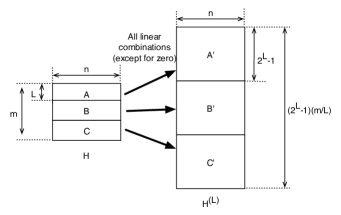
A sub-block of $H$ corresponds to a sub-block in $H^{(L)}$ (for example, sub-block A corresponds to sub-block A’). The row vectors in sub-block X’ (X $\in$ {A,B,C} ) can be obtained by constructing all linear combinations (except for the zero combination) of the row vectors in sub-block X.

Figure 1: Redundant extension of a parity check matrix.

Figure 1 illustrates the idea of the redundant extension.

From the above definition of the redundant extension, it is clear that the row spaces of $H$ and $H^{(L)}$ are the same. In other words, the code defined by $H$ coincides with the code defined by $H^{(L)}$. However, although the codes defined by $H$ and $H^{(L)}$ are the same, $H$ and $H^{(L)}$ may have different SS weight distributions.

Example 3

For a given $m\times n$ matrix $H$, $H^{(2)}$ is expressed as

$$H^{(2)}=\left(\begin{array}[]{c}\mbox{\boldmath$h$}_{1}\\ \mbox{\boldmath$h$}_{2}\\ \mbox{\boldmath$h$}_{1}\oplus\mbox{\boldmath$h$}_{2}\\ \mbox{\boldmath$h$}_{3}\\ \mbox{\boldmath$h$}_{4}\\ \mbox{\boldmath$h$}_{3}\oplus\mbox{\boldmath$h$}_{4}\\ \vdots\\ \mbox{\boldmath$h$}_{m-1}\\ \mbox{\boldmath$h$}_{m}\\ \mbox{\boldmath$h$}_{m-1}\oplus\mbox{\boldmath$h$}_{m}\\ \end{array}\right).$$ (44)

∎

The definition of the redundant extension of a matrix naturally leads to the following definition of the redundant extension of a given ensemble:

Definition 6 (Extended ensemble)

Consider the case where a random ensemble ${\cal G}$ which consists of $m\times n$ binary matrices is given. Let $L$ be a divisor of $m$. The extended ensemble of ${\cal G}$, denoted by ${\cal G}^{(L)}$, is defined by

$${\cal G}^{(L)}\stackrel{{\scriptstyle\triangle}}{{=}}\{H^{(L)}:H\in{\cal G}\}.$$ (45)

The size of the ensemble $\#{\cal G}^{(L)}$ is equal to the size of the original ensemble $\#{\cal G}$. An equal probability is assigned to each matrix in ${\cal G}^{(L)}$. ∎

The redundant random ensemble which is the main subject of this paper is the extended ensemble of a random ensemble, which is denoted by ${\cal R}_{m,n}^{(L)}$.

III-B Redundant random ensemble: $L=2$

In this subsection, we discuss the average SS weight distribution of the redundant random ensemble ${\cal R}_{m,n}^{(2)}$. In this case, we can derive a simple exact formula for the average SS weight distribution.

Suppose that the first 3-rows of $H\in{\cal R}_{m,n}^{(2)}$,

$$\tilde{H}\stackrel{{\scriptstyle\triangle}}{{=}}\left(\begin{array}[]{c}\mbox{\boldmath$h$}_{1}\\ \mbox{\boldmath$h$}_{2}\\ \mbox{\boldmath$h$}_{1}\oplus\mbox{\boldmath$h$}_{2}\\ \end{array}\right),$$ (46)

are given. Our first task is to count the number of pairs $(\mbox{\boldmath$h$}_{1},\mbox{\boldmath$h$}_{2})\in F_{2}^{n}\times F_{2}^{n}$ satisfying $q_{\tilde{H}}(\mbox{\boldmath$x$}_{w})=0$. Let us define $U$ by

$$U\stackrel{{\scriptstyle\triangle}}{{=}}\#\{(\mbox{\boldmath$h$}_{1},\mbox{\boldmath$h$}_{2})\in F_{2}^{n}\times F_{2}^{n}:\mbox{\boldmath$h$}_{1}\circ\mbox{\boldmath$x$}_{w}\neq 1,\mbox{\boldmath$h$}_{2}\circ\mbox{\boldmath$x$}_{w}\neq 1,$$

$$(\mbox{\boldmath$h$}_{1}\oplus\mbox{\boldmath$h$}_{2})\circ\mbox{\boldmath$x$}\neq 1\}.$$ (47)

Note that $m/2$ sub-blocks exist in $H\in{\cal R}_{n,m}^{(2)}$, and these sub-blocks can be chosen independently when we count $\#\{H\in{\cal R}_{n,m}^{(2)}:q_{H}(\mbox{\boldmath$x$}_{w})=0\}$. This observation leads to the following equality,

$$\#\{H\in{\cal R}_{n,m}^{(2)}:q_{H}(\mbox{\boldmath$x$}_{w})=0\}=U^{m/2}.$$ (48)

The next lemma gives a simple description of $U$.

Lemma 7

For $1\leq m<n$, $w\geq 1$, $U$ is given by

$$U=(2^{n}-w2^{n-w})^{2}-2^{2(n-w)+1}\sum_{\gamma=2}^{w}{w\choose\gamma}(w-\gamma).$$ (49)

(Proof) Let

$$V\stackrel{{\scriptstyle\triangle}}{{=}}\#\{(\mbox{\boldmath$h$}_{1},\mbox{\boldmath$h$}_{2})\in F_{2}^{n}\times F_{2}^{n}:\mbox{\boldmath$h$}_{1}\circ\mbox{\boldmath$x$}_{w}\neq 1,\mbox{\boldmath$h$}_{2}\circ\mbox{\boldmath$x$}_{w}\neq 1,$$

$$(\mbox{\boldmath$h$}_{1}\oplus\mbox{\boldmath$h$}_{2})\circ\mbox{\boldmath$x$}_{w}=1\}.$$ (50)

Using the equality

$$\#\{(\mbox{\boldmath$h$}_{1},\mbox{\boldmath$h$}_{2})\in F_{2}^{n}\times F_{2}^{n}:\mbox{\boldmath$h$}_{1}\circ\mbox{\boldmath$x$}_{w}\neq 1,\mbox{\boldmath$h$}_{2}\circ\mbox{\boldmath$x$}_{w}\neq 1\}$$

$$=(2^{n}-w2^{n-w})^{2},$$ (51)

we have

$$U = \{(\mbox{\boldmath$h$}_{1},\mbox{\boldmath$h$}_{2})\in F_{2}^{n}\times F_{2}^{n}:\mbox{\boldmath$h$}_{1}\circ\mbox{\boldmath$x$}_{w}\neq 1,\mbox{\boldmath$h$}_{2}\circ\mbox{\boldmath$x$}_{w}\neq 1\}$$ (52)

$$- V$$

$$= (2^{n}-w2^{n-w})^{2}-V.$$

In the following, we will evaluate $V$. Define $\alpha,\beta,\gamma$ by

$$\alpha \stackrel{{\scriptstyle\triangle}}{{=}} \#\{i\in[1,n]:h_{i}^{(1)}=1,h_{i}^{(2)}=0,x_{i}=1\}$$ (53)

$$\beta \stackrel{{\scriptstyle\triangle}}{{=}} \#\{i\in[1,n]:h_{i}^{(1)}=0,h_{i}^{(2)}=1,x_{i}=1\}$$ (54)

$$\gamma \stackrel{{\scriptstyle\triangle}}{{=}} \#\{i\in[1,n]:h_{i}^{(1)}=1,h_{i}^{(2)}=1,x_{i}=1\},$$ (55)

where $\mbox{\boldmath$h$}_{1}=(h_{1}^{(1)},h_{2}^{(1)},\ldots,h_{n}^{(1)})$ and $\mbox{\boldmath$h$}_{2}=(h_{1}^{(2)},h_{2}^{(2)},\ldots,h_{n}^{(2)})$. Assume that $\mbox{\boldmath$h$}_{1}\circ\mbox{\boldmath$x$}_{w}\neq 1$ and $\mbox{\boldmath$h$}_{2}\circ\mbox{\boldmath$x$}_{w}\neq 1$. In this case, the equality $(\mbox{\boldmath$h$}_{1}\oplus\mbox{\boldmath$h$}_{2})\circ\mbox{\boldmath$x$}_{w}=1$ holds if and only if the following two conditions hold: (i) $(\alpha,\beta)=(1,0)$ or $(\alpha,\beta)=(0,1)$, (ii) $2\leq\gamma\leq w$. Suppose the case $(\alpha,\beta)=(1,0)$. The number of possible pairs $(\mbox{\boldmath$h$}_{1},\mbox{\boldmath$h$}_{2})$ satisfying $\mbox{\boldmath$h$}_{1}\circ\mbox{\boldmath$x$}_{w}\neq 1,\mbox{\boldmath$h$}_{2}\circ\mbox{\boldmath$x$}_{w}\neq 1$, $(\mbox{\boldmath$h$}_{1}\oplus\mbox{\boldmath$h$}_{2})\circ\mbox{\boldmath$x$}_{w}=1$ is given by

$$\sum_{\gamma=2}^{w}{w\choose\gamma}(w-\gamma)2^{2(n-w)}.$$ (56)

Taking the case $(\alpha,\beta)=(0,1)$ into consideration, we immediately have

$$V=2^{2(n-w)+1}\sum_{\gamma=2}^{w}{w\choose\gamma}(w-\gamma).$$ (57)

Substituting this equation into Eq.(52), we obtain the claim of the lemma. ∎

The following theorem is an immediate consequence of Lemma 7.

Theorem 1 (Average SS distribution of ${\cal R}_{m,n}^{(2)}$ )

The average SS weight distribution of ${\cal R}_{m,n}^{(2)}$ is given by

$$S_{w}^{{\cal R}_{m,n}^{(2)}} = \frac{{n\choose w}}{2^{mn}}\left((2^{n}-w2^{n-w})^{2}-V\right)^{m/2}$$ (58)

for $1\leq m<n$, $w\geq 1$, where $V$ is defined by

$$V\stackrel{{\scriptstyle\triangle}}{{=}}2^{2(n-w)+1}\sum_{\gamma=2}^{w}{w\choose\gamma}(w-\gamma).$$ (59)

(Proof) The average SS weight distribution of ${\cal R}_{n,m}^{(2)}$ can be derived in the following way:

$$S_{w}^{{\cal R}_{m,n}^{(2)}} = \frac{1}{\#{\cal R}_{m,n}^{(2)}}\sum_{\mbox{\boldmath$x$}\in Z^{(n,w)}}\#\{H\in{\cal R}_{n,m}^{(2)}:q_{H}(\mbox{\boldmath$x$})=0\}$$ (60)

$$= \frac{{n\choose w}}{2^{mn}}\#\{H\in{\cal R}_{m,n}^{(2)}:q_{H}(\mbox{\boldmath$x$}_{w})=0\}$$

$$= \frac{{n\choose w}}{2^{mn}}U^{m/2}$$

$$= \frac{{n\choose w}}{2^{mn}}\left((2^{n}-w2^{n-w})^{2}-V\right)^{m/2}$$

The second equality follows from the symmetric property of the ensemble, while the third equality is derived from Eq.(48). The last equality is due to Lemma 7. ∎

Example 4

Consider the case where $n=4,m=2$. The ensemble ${\cal R}_{2,4}^{(2)}$ consists of matrices of the form

$$\left(\begin{array}[]{c}\mbox{\boldmath$h$}_{1}\\ \mbox{\boldmath$h$}_{2}\\ \mbox{\boldmath$h$}_{1}\oplus\mbox{\boldmath$h$}_{2}\\ \mbox{\boldmath$h$}_{3}\\ \mbox{\boldmath$h$}_{4}\\ \mbox{\boldmath$h$}_{3}\oplus\mbox{\boldmath$h$}_{4}\\ \end{array}\right).$$ (61)

We consider the case that the row vectors $\mbox{\boldmath$h$}_{1},\mbox{\boldmath$h$}_{2},\mbox{\boldmath$h$}_{3},\mbox{\boldmath$h$}_{4}$ are chosen from $F_{2}^{4}$ with uniform probability. From Theorem 1, we have

$$\left\{S_{w}^{{\cal R}_{2,4}}\right\}_{w=1}^{4}=\left\{1,\frac{3}{2},\frac{19}{16},\frac{7}{16}\right\}.$$ (62)

On the other hand, ${\cal R}_{2,4}$, which is the set of matrices of the form

$$\left(\begin{array}[]{c}\mbox{\boldmath$h$}_{1}\\ \mbox{\boldmath$h$}_{2}\\ \mbox{\boldmath$h$}_{3}\\ \mbox{\boldmath$h$}_{4}\\ \end{array}\right),$$ (63)

has the average SS weight distribution

$$\left\{S_{w}^{{\cal R}_{2,4}}\right\}_{w=1}^{4}=\left\{1,\frac{3}{2},\frac{25}{16},\frac{9}{16}\right\},$$ (64)

where this distribution is derived using Lemma 2. It can be observed that the average SS weights of the extended ensemble are smaller those that of the original ensemble in the cases $w=3$ and $4$. ∎

The argument used in the proof of Theorem 1 can be used to derive the average SS weight distribution of the extended constant row weight ensemble with $L=2$, the details are summarized in the Appendix. Here we consider the following example.

Example 5

Let $n=100,m=50$. The average SS weight distribution of the extended constant row weight ensembles with $L=2$, $S_{w}^{{\cal C}_{100,50,r}^{(2)}}$, can be evaluated using Lemma 13 of the Appendix. Tables I and II present the two cases $r=10$ (sparse matrix) and $r=50$ (dense matrix), respectively. We can see that the improvement due to extension is very small for the case $r=10$. On the other hand, a significant improvement can be observed for the case $r=50$. ∎

TABLE I: Comparison of a non-extended ensemble and an extended ensemble(constant row weight ensemble, sparse case).

$w$	$S_{w}^{{\cal C}_{n,m,r}}$	$S_{w}^{{\cal C}_{n,m,r}^{(2)}}$
1	0.515	0.515
2	0.217	0.217
3	0.107	0.107
4	0.0726	0.0721
5	0.0748	0.0737
6	0.123	0.119
7	0.322	0.308
8	1.33	1.24
9	8.20	7.54
10	71.5	64.6

$n=100,m=50,r=10$

TABLE II: Comparison of a non-extended ensemble and an extended ensemble(constant row weight ensemble, dense case).

$w$	$S_{w}^{{\cal C}_{n,m,r}}$	$S_{w}^{{\cal C}_{n,m,r}^{(2)}}$
1	$8.88\times 10^{-14}$	$8.88\times 10^{-14}$
2	$2.65\times 10^{-12}$	$2.65\times 10^{-12}$
3	$7.43\times 10^{-6}$	$8.32\times 10^{-9}$
4	$2.23\times 10^{0}$	$4.18\times 10^{-3}$
5	$1.87\times 10^{4}$	$3.08\times 10^{2}$

$n=100,m=50,r=50$

This example suggests that the advantages of redundant extension are more significant when the original matrix is dense. This is one of the major reasons that we focus on redundant random ensembles in the present study.

III-C Redundant random ensemble: $L>2$

It becomes difficult to evaluate the number of extended parity check matrices giving a stopping set for a given weight when $L>2$.Instead of deriving an exact expression, we here utilize upper and lower bounds on the number of such parity check matrices to study the average SS weight distribution of extended ensembles.

III-C1 Number of generator matrices with minimum distance greater than or equal to 2

Let $G$ be a binary $K\times N$ matrix($1\leq K<N$). The weight distribution of the code generated from $G$ (as a generator matrix) is defined by

$$A_{w}(G)\stackrel{{\scriptstyle\triangle}}{{=}}\sum_{\mbox{\boldmath$c$}\in Z^{(N,w)}}\sum_{\mbox{\boldmath$m$}\in\bar{F}_{2}^{K}}I[\mbox{\boldmath$m$}G=\mbox{\boldmath$c$}]$$ (65)

for $1\leq w\leq N$, where $\bar{F}_{2}^{K}$ denotes $F_{2}^{K}\backslash\mbox{\boldmath$0$}$. The average of the weight distribution (where expectation is taken over a given ensemble ${\cal G}$) is given by

$$E_{\cal G}[A_{w}(G)] = \sum_{G\in{\cal G}}P(G)\sum_{\mbox{\boldmath$c$}\in Z^{(N,w)}}\sum_{\mbox{\boldmath$m$}\in\bar{F}_{2}^{K}}I[\mbox{\boldmath$m$}G=\mbox{\boldmath$c$}]$$ (66)

$$= \frac{1}{\#{\cal G}}\sum_{\mbox{\boldmath$c$}\in Z^{(N,w)}}\sum_{\mbox{\boldmath$m$}\in\bar{F}_{2}^{K}}\#\{G\in{\cal G}:\mbox{\boldmath$m$}G=\mbox{\boldmath$c$}\}.$$ (67)

The minimum distance of $G$ is given by

$$d_{min}(G)\stackrel{{\scriptstyle\triangle}}{{=}}\min\{i\in[1,n]:A_{i}(G)\neq 0\}.$$ (68)

In order to prove the upper and lower bounds on the number of certain parity check matrices, we can use the first and second moment method[7], which requires the first and second moments of a random variable. The following lemma is presented in the problem section of [6] (the proof is given in the Appendix).

Lemma 8

The first and second moments of $A_{w}(G)$ with respect to ${\cal R}_{K,N}$ are given by

$$E_{{\cal R}_{K,N}}[A_{w}(G)]=(2^{K}-1)2^{-N}{N\choose w}$$ (69)

and

$$E_{{\cal R}_{K,N}}[A_{w}(G)^{2}] = E_{{\cal R}_{K,N}}[A_{w}(G)]^{2}+E_{{\cal R}_{K,N}}[A_{w}(G)]$$ (70)

$$\times \left(1-{N\choose w}2^{-N}\right)$$

respectively, for $w\in[1,n]$. ∎

The next lemma is the basis of the lower bound on the average SS weight distribution for redundant random ensembles.

Lemma 9

The number of matrices in ${\cal R}_{K,N}$ which have minimum distance greater than or equal to 2 has a lower bound given by

$$\#\{G\in{\cal R}_{K,N}:d_{min}(G)\geq 2\}\hskip 113.81102pt$$

$$\geq\max\{2^{KN}\max\{1-(2^{K}-1)2^{-N}N,0\},2^{KN-K}\}.$$ (71)

(Proof) Let $D\stackrel{{\scriptstyle\triangle}}{{=}}\#\{G\in{\cal R}_{K,N}:d_{min}(G)\geq 2\}$. We first prove $D\geq 2^{KN}\max\{1-(2^{K}-1)2^{-N}N,0\}$. The number of matrices whose minimum distance is greater than or equal to 2 can be written in the form

$$D = \#\{G\in{\cal R}_{K,N}:A_{1}(G)=0\}$$ (72)

$$= \#\{G\in{\cal R}_{K,N}:A_{1}(G)<1\}$$

$$= \sum_{G\in{\cal R}_{K,N}}I[A_{1}(G)<1]$$

$$= 2^{KN}\sum_{G\in{\cal R}_{K,N}}P(G)I[A_{1}(G)<1]$$

$$= 2^{KN}Pr[A_{1}(G)<1],$$

where $Pr[A_{1}(G)<1]$ is given by

$$Pr[A_{1}(G)<1]=\sum_{G\in{\cal R}_{K,N}}P(G)I[A_{1}(G)<1].$$ (73)

The Markov inequality implies

$$Pr[A_{1}(G)\geq 1]\leq E_{{\cal R}_{K,N}}[A_{1}(G)],$$ (74)

which is equivalent to

$$Pr[A_{1}(G)<1]\geq\max\{1-E_{{\cal R}_{K,N}}[A_{1}(G)],0\}.$$ (75)

Substituting this upper bound into Eq.(72) and using Eq.(69), we have

$$D \geq 2^{KN}\max\{1-E_{{\cal R}_{K,N}}[A_{1}(G)],0\}$$ (76)

$$= 2^{KN}\max\{1-(2^{K}-1)2^{-N}N,0\}.$$

We then consider the inequality $D\geq 2^{KN-K}$. Suppose the case that every row of $G^{\prime}\in{\cal R}_{K,N}$ is of even weight. We call this condition the even weight condition. In such a case, no linear combination of rows of $G^{\prime}$ gives a vector of weight 1. The number of $K\times N$ matrices satisfying the even weight condition is $2^{K(N-1)}$ because there exist $2^{N-1}$ even weight vectors of length $N$. ∎

The next lemma will be required to prove an upper bound on the average SS weight distribution of redundant random ensembles.

Lemma 10

The number of matrices in ${\cal R}_{K,N}$ which have minimum distance greater than or equal to 2 has an upper bound given by

$$\#\{G\in{\cal R}_{K,N}:d_{min}(G)\geq 2\}\hskip 113.81102pt$$

$$\leq 2^{KN}\frac{1-N2^{-N}}{(2^{K}-1)N2^{-N}+1-N2^{-N}}.$$ (77)

(Proof) For a non-negative integer-valued random variable $X$, the following inequality holds[7],

$$Pr[X=0]\leq\frac{E[X^{2}]-E[X]^{2}}{E[X^{2}]}.$$

Considering $A_{1}(G)$ as a random variable, we obtain

$$\#\{G\in{\cal R}_{K,N}:d_{min}(G)\geq 2\}\hskip 170.71652pt$$

$$= \#\{G\in{\cal R}_{K,N}:A_{1}(G)=0\}$$ (78)

$$= 2^{KN}Pr[A_{1}(G)=0]$$

$$\leq 2^{KN}\frac{E_{{\cal R}_{K,N}}[A_{1}(G)^{2}]-E_{{\cal R}_{K,N}}[A_{1}(G)]^{2}}{E_{{\cal R}_{K,N}}[A_{1}(G)^{2}]}.$$

From Lemma 8, the first and the second moments of $A_{1}(G)$ are given by

$$E_{{\cal R}_{K,N}}[A_{1}(G)] = (2^{K}-1)N2^{-N},$$ (79)

$$E_{{\cal R}_{K,N}}[A_{1}(G)^{2}] = ((2^{K}-1)N2^{-N})^{2}$$ (80)

$$+ (2^{K}-1)N2^{-N}\left(1-N2^{-N}\right).$$

Substituting these expressions into Eq.(78), we have the claim of the lemma. ∎

III-C2 Upper and lower bounds on average SS weight distributions

We are now ready to prove the following upper and lower bounds on the average SS weight distribution.

Theorem 2 (Upper and lower bounds on $S_{w}^{{\cal R}_{m,n}^{(L)}}$ )

The average SS weight distribution of the redundant random ensemble satisfies the inequalities

$$S_{w}^{{\cal R}_{m,n}^{(L)}} \geq {n\choose w}\max\{A^{m/L},2^{-m}\}$$ (81)

$$S_{w}^{{\cal R}_{m,n}^{(L)}} \leq {n\choose w}\left(\frac{1-w2^{-w}}{(2^{L}-1)w2^{-w}+1-w2^{-w}}\right)^{m/L}$$ (82)

for $1\leq w\leq n$, where $A$ is defined by

$$A\stackrel{{\scriptstyle\triangle}}{{=}}\max\{1-(2^{L}-1)2^{-w}w,0\}.$$ (83)

(Proof) From the definition of the average SS weight distribution, $S_{w}^{{\cal R}_{m,n}^{(L)}}$ can be expressed as

$$S_{w}^{{\cal R}_{m,n}^{(L)}} = \frac{1}{2^{mn}}\sum_{\mbox{\boldmath$x$}\in Z^{(n,w)}}\#\{H\in{\cal R}_{m,n}^{(L)}:q_{H}(\mbox{\boldmath$x$})=0\}$$ (84)

$$= \frac{1}{2^{mn}}{n\choose w}\#\{H\in{\cal R}_{m,n}^{(L)}:q_{H}(\mbox{\boldmath$x$})=0\}$$

$$= \frac{1}{2^{mn}}{n\choose w}\left(\#\{H^{\prime}\in{\cal R}_{L,n}^{(L)}:q_{H}(\mbox{\boldmath$x$})=0\}\right)^{m/L}$$

$$= \frac{1}{2^{mn}}{n\choose w}$$

$$\times \left(\#\{G\in{\cal R}_{L,w}:d_{min}(G)\geq 2\}2^{L(n-w)}\right)^{m/L},$$

where, in the above, the second equality was obtained by using the symmetric property of the ensemble, and the third equality arises from the property that $L$ sub-blocks can be chosen independently. The last equality holds because

$$\#\{H^{\prime}\in{\cal R}_{L,n}^{(L)}:q_{H^{\prime}}(\mbox{\boldmath$x$})=0\}\hskip 113.81102pt$$

$$=\#\{G\in{\cal R}_{L,w}:d_{min}(G)\geq 2\}2^{L(n-w)}.$$ (85)

Note that $d_{min}(G)\geq 2$ means that no linear combination of row vectors of $G$ (except for all zero coefficients) has weight 1. Applying the inequality in Lemma 10 to Eq.(84), we immediately obtain the upper bound,

$$S_{w}^{{\cal R}_{m,n}^{(L)}} = \frac{1}{2^{mn}}{n\choose w}$$ (86)

$$\times \left(\#\{G\in{\cal R}_{L,w}:d_{min}(G)\geq 2\}2^{L(n-w)}\right)^{m/L}$$

$$\leq \frac{1}{2^{mn}}{n\choose w}\left(2^{Lw}\times B\times 2^{L(n-w)}\right)^{m/L}$$

$$= \frac{1}{2^{mn}}{n\choose w}\left(B\times 2^{Ln}\right)^{m/L}$$

$$= {n\choose w}B^{m/L},$$

where $B$ is defined by

$$B=\frac{1-w2^{-w}}{(2^{L}-1)w2^{-w}+1-w2^{-w}}.$$ (87)

On the other hand, applying the inequality in Lemma 9 to Eq.(86), the lower bound can be derived. Let $D^{\prime}\stackrel{{\scriptstyle\triangle}}{{=}}\#\{G\in{\cal R}_{K,N}:d_{min}(G)\geq 2\}$. The lower bound in Lemma 9 is equivalent to

$$D^{\prime}\geq\max\{2^{Lw}A,2^{Lw-L}\},$$ (88)

which leads to the lower bound

$$S_{w}^{{\cal R}_{m,n}^{(L)}} = \frac{1}{2^{mn}}{n\choose w}\left(D^{\prime}2^{L(n-w)}\right)^{m/L}$$ (89)

$$\geq \frac{1}{2^{mn}}{n\choose w}\left(\max\{2^{Lw}A,2^{Lw-L}\}2^{L(n-w)}\right)^{m/L}$$

$$= {n\choose w}\max\{A^{m/L},2^{-m}\}.$$

∎

It is easy to check that the upper bound and the lower bound coincide with the average SS weight distribution of the non-extended ensemble $S_{w}^{{\cal R}_{m,n}}$ given in Eq. (12) if $L=1$.

Example 6

Consider the case $n=100,m=50,L=2$. In this case, we can compute exact values of the average SS weight distribution due to Theorem 1. Table III presents the exact values (Theorem 1) together with the values of the upper and lower bound(Theorem 2) of the average SS weight distribution of ${\cal R}_{50,100}^{(2)}$. For the cases $w=1$ and $2$, we can see that the values of the upper and lower bounds coincide and they give the exact values.

TABLE III: Average SS weight distribution $S_{w}^{{\cal R}_{50,100}^{(2)}}$: exact, upper and lower bounds.

$w$	Exact	Upper	Lower
1	$8.88\times 10^{-14}$	$8.88\times 10^{-14}$	$8.88\times 10^{-14}$
2	$4.40\times 10^{-12}$	$4.40\times 10^{-12}$	$4.40\times 10^{-12}$
3	$1.05\times 10^{-8}$	$1.07\times 10^{-6}$	$1.44\times 10^{-10}$
4	$4.15\times 10^{-3}$	$1.17\times 10^{-1}$	$3.48\times 10^{-9}$
5	$2.58\times 10^{2}$	$1.20\times 10^{3}$	$1.02\times 10^{1}$

∎

An exact ( non-trivial) expression for $S_{w}^{{\cal R}_{m,n}^{(L)}}(L>2)$ does not at present exist. Let $Q_{L,w}\stackrel{{\scriptstyle\triangle}}{{=}}\#\{G\in{\cal R}_{L,w}:d_{min}(G)\geq 2\}$. The source of the difficulty in deriving an exact expression comes from the difficulty in counting $Q_{L,w}$ precisely. However, if both $L$ and $w$ are small, we can obtain $Q_{L,w}$ by an exhaustive computer search. Table IV presents the values of $Q_{L,w}$ for $1\leq w,L\leq 5$ which have been evaluated by such an exhaustive computer search.

TABLE IV: Values of $Q_{L,w}$(The number of matrices with minimum distance greater than or equal to 2).

$L\backslash w$	1	2	3	4	5
1	1	2	5	12	27
2	1	4	19	112	619
3	1	8	71	792	10683
4	1	16	271	5416	140251
5	1	32	1055	38472	1751067

The following lemma gives exact value of $S_{w}^{{\cal R}_{m,n}^{(L)}}$ if we know the value of $Q_{L,w}$.

Lemma 11

The average SS weight distribution of ${\cal R}_{m,n}^{(L)}$ is given by

$$S_{w}^{{\cal R}_{m,n}^{(L)}}=\frac{1}{2^{mn}}{n\choose w}\left(Q_{L,w}2^{L(n-w)}\right)^{m/L}.$$ (90)

(Proof) The claim of the lemma has already been derived as Eq.(84). ∎

Example 7

Consider the case $n=100,m=50,L=5$. Combining Lemma 11 and the result presented in Table IV, we can derive the exact values of the average SS weight distribution for $1\leq w,L\leq 5$. These values are presented in Table V together with the corresponding values of the upper and lower bounds.

TABLE V: Average SS weight distribution $S_{w}^{{\cal R}_{50,100}^{(5)}}$: exact, upper and lower bounds.

$w$	Exact	Upper	Lower
1	$8.88\times 10^{-14}$	$8.88\times 10^{-14}$	$8.88\times 10^{-14}$
2	$4.40\times 10^{-12}$	$4.40\times 10^{-12}$	$4.40\times 10^{-12}$
3	$1.94\times 10^{-10}$	$1.93\times 10^{-8}$	$1.44\times 10^{-10}$
4	$1.73\times 10^{-8}$	$1.12\times 10^{-4}$	$3.48\times 10^{-9}$
5	$1.13\times 10^{-5}$	$3.89\times 10^{-1}$	$6.69\times 10^{-8}$

∎

There is a trade-off between the extension degree $L$ and the average SS weight distribution. The decoding complexity of BP-based iterative decoding increases as $L$ increases because the number of rows in the extended matrix $(2^{L}-1)(m/L)$ is an exponentially increasing function of $L$. On the other hand, a large $L$ tends to give a larger stopping distance. The next example demonstrates such a trade off relation.

Example 8

Figure 2 presents the relation between $L$ and the upper bound of the average SS weight distribution. The horizontal axis of Fig.2 represents the weight $w$. The ensemble assumed here is the random ensemble with $n=100,m=50$, namely ${\cal R}_{50,100}$. We can observe that the upper bound on the average SS weight distribution decreases as $L$ increases for a fixed weight.

$n=100$, $m=50$

Figure 2: Upper bounds on the average SS weight distribution of redundant random ensembles.

∎

Example 9

Figure 3 shows the block error probability of three example ensembles with $m=50,n=100$: the random ensemble (matrix A) , the redundant random ensemble with $L=2$ (matrix B) and the redundant random ensemble with $L=5$(matrix C). The channel is BEC and BP is used in the decoder. It is observed that the decoding performance of matrix C is the best among the three matrices. The reason for these differing performances can be seen with reference to Table VI. This table presents the stopping distance of the three matrices and their multiplicity. The multiplicity is the number of the stopping sets with size equal to the stopping distance. These values have been computed by an exhaustive computer search. The matrix C has the largest stopping distance, 7, which gives a smaller block error probability compared with those of matrices A(stopping distance 4) and B(stopping distance 5).

$n=100$, $m=50$

Figure 3: Block error probabilities of examples of random and redundant random ensembles (Matrices A,B, and C from top to bottom).

TABLE VI: Stopping distance and multiplicity of matrices A,B and C.

$n=100,m=50$

Matrix	$L$	Stopping distance	Multiplicity	# of rows
A	1	4	1	50
B	2	5	262	75
C	5	7	1365	310

∎

III-D Typical stopping distance

From the average SS weight distribution, we can retrieve some information about the stopping distance of matrices contained in an ensemble.

Definition 7 (Typical stopping distance)

The typical stopping distance of an ensemble ${\cal G}$ is defined by

$$\delta^{{\cal G}}\stackrel{{\scriptstyle\triangle}}{{=}}\min\left\{s\in[1,n]:\sum_{w=1}^{s-1}S_{w}^{{\cal G}}\geq 1\right\}.$$ (91)

∎

The condition $\sum_{w=1}^{s-1}S_{w}(H)=0$ is equivalent to $\Delta(H)\geq s$. It is evident that there exists a matrix $H\in{\cal G}$ satisfying $\sum_{w=1}^{\delta^{{\cal G}}-1}S_{w}(H)=0$, because the average $\sum_{w=1}^{\delta^{{\cal G}}-1}S_{w}^{{\cal G}}$ is strictly smaller than 1. This means that there exists a matrix with a stopping distance larger than or equal to the typical stopping distance $\delta^{{\cal G}}$.

We here compare a high rate redundant random ensemble with constant row weight ensembles and bipartite ensembles in terms of their typical stopping distances.

Example 10

Consider the case $n=1024,m=32$. We can show that the maximum value of the typical stopping distance of ${\cal C}_{n,m,r}$ is

$$\max_{r\in[1,1024]}\delta^{{\cal C}_{1024,32,r}}=3.$$

For bipartite ensembles, we have

$$\max_{c\geq 3}\delta^{{\cal B}_{c,32c}}=3.$$

These results mean that there are no constant row weight ensembles and bipartite ensembles with $n=1024,m=32$ which achieve the typical stopping distance 4. On the other hand, the redundant random ensemble $(n=1024,m=32,L=8)$ has a larger typical stopping distance:

$$\delta^{{\cal R}_{32,1024}^{(8)}}=4.$$

In this case, the extended random ensemble is expected to give asymptotically (i.e., in the regime of small erasure probability) better decoding performance (with BP) than the constant row weight ensemble with any row weight and the bipartite ensemble.

Figure 4 presents the block error probabilities of examples of a redundant random ensemble ($n=1024,m=32,L=4,8$) and a constant row weight ensemble ($n=1024,m=32,r=100,200,300)$. Note that the size of the parity check matrices used in the BP decoder is $120\times 1024$ (redundant random, $L=4$), $1020\times 1024$ (redundant random, $L=8$), $32\times 1024$ (constant row weight), respectively. It may be observed that the example redundant random ensembles give steeper error curves than those of the example constant row weight ensembles. This difference in decoding performance could be explained from the the difference in typical stopping distance discussed above. ∎

$n=1000$, $m=32$

Figure 4: Block error probabilities (BP on BEC) of examples of a redundant random ensemble and constant row weight ensemble.

IV Asymptotic growth rate of the average SS weight distributions of redundant random ensembles

In this section, we will discuss the asymptotic (i.e., in the limit as $n$ goes to infinity) behavior of the average SS weight distribution.

IV-A Bounds on asymptotic growth rate

We will consider the asymptotic behavior of the average SS weight distribution of the redundant random ensembles.

The asymptotic growth rate $\sigma_{\ell}(R,\mu)$ is defined by

$$\sigma_{\ell}(R,\mu)\stackrel{{\scriptstyle\triangle}}{{=}}\lim_{n\rightarrow\infty}\frac{1}{n}\log S_{\ell n}^{{\cal R}_{(1-R)n,n}^{(\mu n)}},$$ (92)

for $0\leq\ell\leq 1,0<\mu\leq 1-R$. The parameter $\mu$ is called normalized extension degree. It is evident that, from the definition of redundant extension, the above definition of $\sigma_{\ell}(R,\mu)$ is well defined only if $(1-R)/\mu$ is an integer.

The next corollary gives a lower bound on $\sigma_{\ell}(R,\mu)$.

Corollary 1

The asymptotic growth rate $\sigma_{\ell}(R,\mu)$ can be lower bounded by

$$\sigma_{\ell}(R,\mu)\geq\left\{\begin{array}[]{ll}H(\ell)-(1-R),&\ell\leq\mu\\ H(\ell),&\ell>\mu.\end{array}\right.$$ (93)

(Proof) We first consider the case $\ell\leq\mu$. From Theorem 2, we have the following inequality,

$$S_{\ell n}^{{\cal R}_{(1-R)n,n}^{(\mu n)}}\geq\max\{A^{\prime(1-R)/\mu},2^{-(1-R)n}\}{n\choose\ell n},$$ (94)

where

$$A^{\prime}\stackrel{{\scriptstyle\triangle}}{{=}}\max\{1-(2^{\mu n}-1)2^{-\ell n}\ell n,0\}.$$ (95)

It is evident that $1-(2^{\mu n}-1)2^{-\ell n}\ell n\rightarrow-\infty$ in the limit as $n$ goes to infinity. This implies the equality

$$\max\{A^{\prime(1-R)/\mu},2^{-(1-R)n}\}=2^{-(1-R)n}$$ (96)

holds for sufficiently large $n$. Upon using this result, we immediately obtain a lower bound,

$$\sigma_{\ell}(R,\mu) = \lim_{n\rightarrow\infty}\frac{1}{n}\log S_{\ell n}^{{\cal R}_{(1-R)n,n}^{(\mu n)}}$$ (97)

$$\geq \lim_{n\rightarrow\infty}\frac{1}{n}\log 2^{-(1-R)n}{n\choose\ell n}$$

$$= H(\ell)-(1-R).$$

We next consider the case $\ell>\mu$. In this case, $1-(2^{\mu n}-1)2^{-\ell n}\ell n\rightarrow 1$ in the limit as $n$ goes to infinity, and so

$$\max\{A^{\prime(1-R)/\mu},2^{-(1-R)n}\}\rightarrow 1$$ (98)

in the limit as $n\rightarrow\infty$. Upon using this result, we obtain

$$\sigma_{\ell}(R,\mu) = \lim_{n\rightarrow\infty}\frac{1}{n}\log S_{\ell n}^{{\cal R}_{(1-R)n,n}^{(\mu n)}}$$ (99)

$$\geq \lim_{n\rightarrow\infty}\frac{1}{n}\log{n\choose\ell n}$$

$$= H(\ell).$$

∎

The next corollary provides an upper bound on $\sigma_{\ell}(R,\mu)$.

Corollary 2

The asymptotic growth rate $\sigma_{\ell}(R,\mu)$ has an upper bound given by

$$\sigma_{\ell}(R,\mu)\leq\left\{\begin{array}[]{ll}H(\ell)-(1-R)\left(1-\frac{\ell}{\mu}\right),&\ell\leq\mu\\ H(\ell),&\ell>\mu.\end{array}\right.$$ (100)

(Proof) The upper bound in Theorem 2 can be rewritten in the form

$$S_{\ell n}^{{\cal R}_{(1-R)n,n}^{(\mu n)}} \leq \left(\frac{1-\ell n2^{-\ell n}}{2^{\mu n}\ell n2^{-\ell n}+1-2\ell n2^{-\ell n}}\right)^{(1-R)/\mu}{n\choose\ell n}$$ (101)

$$\leq \left(\frac{1-\ell n2^{-\ell n}}{2^{(\mu-\ell)n}\ell n}\right)^{(1-R)/\mu}{n\choose\ell n}$$

for sufficiently large $n$. The last inequality holds because $1-2\ell n2^{-\ell n}$ is always positive for large $n$. Thus, the asymptotic growth rate can be bounded from above:

$$\sigma_{\ell}(R,\mu) \leq H(\ell)+\frac{(1-R)}{\mu}\lim_{n\rightarrow\infty}\frac{1}{n}\log\frac{1-\ell n2^{-\ell n}}{2^{(\mu-\ell)n}\ell n}$$ (102)

$$= H(\ell)+\frac{(1-R)}{\mu}$$

$$\times \lim_{n\rightarrow\infty}\frac{1}{n}\left(\log(1-\ell n2^{-\ell n})-\log(2^{(\mu-\ell)n})-\log(\ell n)\right)$$

$$= H(\ell)+\frac{(1-R)}{\mu}\lim_{n\rightarrow\infty}\frac{1}{n}\left(-(\mu-\ell)n\right)$$

$$= H(\ell)-(1-R)\left(1-\frac{\ell}{\mu}\right).$$

On the other hand, the inequality

$$\frac{1-\ell n2^{-\ell n}}{(2^{\mu n}-1)\ell n2^{-\ell n}+1-\ell n2^{-\ell n}}\leq 1$$ (103)

leads to another (trivial) upper bound on $S_{\ell n}^{{\cal R}_{(1-R)n,n}^{(\mu n)}}$,

$$S_{\ell n}^{{\cal R}_{(1-R)n,n}^{(\mu n)}}\leq{n\choose\ell n}.$$ (104)

The asymptotic form of this upper bound is given by

$$\sigma_{\ell}(R,\mu)\leq H(\ell).$$ (105)

If $\ell<\mu$, the upper bound (102) gives smaller values than the trivial bound (105). If $\ell>\mu$, the trivial bound (105) becomes tighter. When $\ell=\mu$, both of the bounds yield the same value $H(\ell)$. ∎

Combining the above two corollaries, we can see that $\sigma_{\ell}(R,\mu)=H(\ell)$ for $\ell>\mu$. That is, the upper and lower bounds are asymptotically tight when $\ell>\mu$.

Example 11

Figure 5 shows the lower bound (Corollary 1) and the upper bound (Corollary 2) for the case $R=0.5$, $\mu=0.25$. The horizontal axis of Fig.5 represents the normalized weight $\ell$. The curve $H(\ell)$ (the asymptotic growth rate of non-extended ensemble ${\cal R}_{(1-R)n,n}$) is also included in Fig.5 as a reference.

Figure 5: Upper and lower bounds on the asymptotic growth rate of the redundant random ensemble ($R=0.5$, $\mu=0.25$).

IV-B Critical exponent

The critical exponent of an ensemble is the normalized weight such that the asymptotic growth rate changes from negative to positive. The explicit definition of the critical exponent of a redundant random ensemble is given below:

Definition 8 (Critical exponent)

The critical exponent of the redundant random ensemble is defined by

$$\alpha(R,\mu)\stackrel{{\scriptstyle\triangle}}{{=}}\inf\{\ell>0:\sigma_{\ell}(R,\mu)\geq 0\}.$$ (106)

∎

The following lemma, which gives bounds on the critical exponent, is a direct consequence of Corollaries 1 and 2.

Lemma 12

The following inequality holds

$$\alpha_{L}(R,\mu)\leq\alpha(R,\mu)\leq\alpha_{U}(R,\mu),$$ (107)

where $\alpha_{L}(R,\mu)$ is the minimum positive solution of $H(\ell)-(1-R)(1-\ell/\mu)=0,$ and $\alpha_{U}(R,\mu)$ is the minimum positive solution of $H(\ell)-(1-R)=0.$
(Proof) From Corollaries 1 and 2, it is evident that the claim holds. ∎

The critical exponent of the bipartite ensemble is given by[2],

$$\beta(c,d)\stackrel{{\scriptstyle\triangle}}{{=}}\inf\{\ell>0:\gamma_{\ell}(c,d)\geq 0\}.$$ (108)

Figure 6 presents the lower bound on the critical exponent of the redundant random ensemble with $R=0.5$ and $R=0.75$. The horizontal axis is the normalized extension degree $\mu$. Of course, if $(1-R)/\mu$ is not an integer, the lower bound is not well defined. However, for simplicity, the lower bound is plotted as if it were valid in the entire range $0<\mu\leq 1-R$. We can see that the exponent increases as $\mu$ increases. Since the parameter $\mu$ can be considered as a measure of decoding complexity, the plots in Fig. 6 can be regarded as the trade-off curves between decoding complexity and the asymptotic decoding performance.

Figure 6: Upper bounds on the critical exponent of redundant random ensembles ($R=0.5,0.75$).

We then compare the critical exponent of the redundant random ensemble and the bipartite ensemble with a design rate of 0.5. It is known that there exists an optimal choice of the variable node degree $c$ to attain the maximum critical exponent $\beta(c,d)$. The best value is $\max_{c\geq 3}\beta(c,2c)=0.065,$ which is obtained when $c=7,d=14$. In other words, no bipartite ensemble with $R=0.5$ yields a critical exponent larger than $0.065$. Note that the plot of the lower bound on the critical exponent of the redundant random ensemble takes larger values than $0.065$ if $\mu$ is sufficiently large. This result implies that the asymptotic BP-performance on BEC of a dense matrix can be better than that of a sparse matrix.

In the case of a high code rate (design rate $R=0.75$), we have $\max_{c}\beta(c,4c)=0.027$. The maximum value is obtained when $c=9,d=36$. We can observe that, as for the former case, the redundant random ensemble with sufficiently large $\mu$ gives larger values.

Example 12

Figure 7 presents the asymptotic growth rate of the random ensemble ($R=0.5$), bipartite ensemble $(c=7,d=14)$, constant row weight ensemble ($R=0.5,r=15$) and the redundant random ensemble ($R=0.5,\mu=0.5$, upper bound). The parameters of the bipartite ensemble and the constant row weight ensemble are chosen so as to maximize the critical exponent under the constraint $R=0.5$. In this case, both the bipartite and the constant row weight ensembles have almost the same maximum critical exponent of 0.065. On the other hand, we have $\alpha_{L}(0.5,0.5)=0.083$, which is larger than the maximum critical exponent of the constant row weight ensemble and the bipartite ensemble. ∎

Figure 7: Comparison of the asymptotic growth rates: random, bipartite, constant row weight, and redundant random ensembles.

V Conclusion

In this paper, the average SS weight distribution and the asymptotic growth rate of redundant random ensembles have been analyzed. The results obtained in the paper describe one aspect of the trade-off between decoding complexity of BP(extension degree) and decoding performance. It is shown that, in some cases, a dense matrix with linearly dependent rows can yield a better decoding performance over BEC than a regular LDPC matrix with comparable parameters. In particular, in the high rate regime, a redundant matrix appears to offer promising performance not only for BEC, but also for other channels. It is hoped that further research concerning this result can be undertaken.

Appendix

Proof of the first and second moment of $A_{w}(G)$

From a simple counting argument, we obtain $\#\{G\in{\cal R}_{K,N}:\mbox{\boldmath$m$}G=\mbox{\boldmath$c$}\}=2^{(K-1)N}$. This equation leads to the transformation

$$E_{{\cal R}_{K,N}}[A_{w}(G)] = \frac{1}{2^{KN}}$$ (109)

$$\times \sum_{\mbox{\boldmath$c$}\in Z^{(N,w)}}\sum_{\mbox{\boldmath$m$}\in\bar{F}_{2}^{K}}\#\{G\in{\cal R}_{K,N}:\mbox{\boldmath$m$}G=\mbox{\boldmath$c$}\}$$

$$= \frac{{N\choose w}}{2^{KN}}\sum_{\mbox{\boldmath$m$}\in\bar{F}_{2}^{K}}\#\{G\in{\cal R}_{K,N}:\mbox{\boldmath$m$}G=\mbox{\boldmath$c$}\}$$

$$= \frac{{N\choose w}}{2^{KN}}(2^{K}-1)2^{(K-1)N}$$

$$= {N\choose w}(2^{K}-1)2^{-N}.$$

We next consider the second moment. The second moment can be written as

$$E_{{\cal R}_{K,N}}[(A_{w}(G))^{2}]\hskip 142.26378pt$$

$$= \sum_{\mbox{\boldmath$c$}_{1},\mbox{\boldmath$c$}_{2}\in Z^{(N,w)}}\sum_{\mbox{\boldmath$m$}_{1},\mbox{\boldmath$m$}_{2}\in\bar{F}_{2}^{K}}I[\mbox{\boldmath$m$}_{1}G=\mbox{\boldmath$c$}_{1},\mbox{\boldmath$m$}_{2}G=\mbox{\boldmath$c$}_{2}]$$ (110)

$$= \sum_{\mbox{\boldmath$c$}_{1},\mbox{\boldmath$c$}_{2}}\sum_{\mbox{\boldmath$m$}_{1},\mbox{\boldmath$m$}_{2}}I[\mbox{\boldmath$m$}_{1}\neq\mbox{\boldmath$m$}_{2}]X_{1}$$

$$+ \sum_{\mbox{\boldmath$c$}_{1},\mbox{\boldmath$c$}_{2}}\sum_{\mbox{\boldmath$m$}_{1},\mbox{\boldmath$m$}_{2}}I[\mbox{\boldmath$m$}_{1}=\mbox{\boldmath$m$}_{2}]I[\mbox{\boldmath$c$}_{1}\neq\mbox{\boldmath$c$}_{2}]X_{2}$$

$$+ \sum_{\mbox{\boldmath$c$}_{1},\mbox{\boldmath$c$}_{2}}\sum_{\mbox{\boldmath$m$}_{1},\mbox{\boldmath$m$}_{2}}I[\mbox{\boldmath$m$}_{1}=\mbox{\boldmath$m$}_{2}]I[\mbox{\boldmath$c$}_{1}=\mbox{\boldmath$c$}_{2}]X_{3}$$

From a combinatorial argument, we have $X_{1}=2^{-2N},X_{2}=0,X_{3}=2^{-N}$. Finally, we get

$$E_{{\cal R}_{K,N}}[(A_{w}(G))^{2}]\hskip 142.26378pt$$

$$= {N\choose w}^{2}\left((2^{K}-1)^{2}-(2^{K}-1)\right)2^{-2N}$$ (111)

$$+ {N\choose w}(2^{K}-1)2^{-N}$$

$$= \left(E_{{\cal R}_{K,N}}[A_{w}(G)]\right)^{2}$$

$$+ E_{{\cal R}_{K,N}}[A_{w}(G)]\left(1-{N\choose w}2^{-N}\right).$$

Redundant constant row weight ensemble: $L=2$

As in the case of the redundant random ensemble, it is possible to write down a simple formula for the redundant constant row weight ensembles if $L=2$.

Lemma 13

The average SS weight distribution of the redundant constant row weight ensemble with parameters $n,m(1\leq m<n),r(r\geq 1)$ and $L=2$ is given by

$$S_{w}^{{\cal C}_{n,m,r}^{(2)}}=\frac{{n\choose w}}{{n\choose r}^{m}}\left(\left({n\choose r}-w{n-w\choose r-1}\right)^{2}-V\right)^{m/2},$$ (112)

where $V$ is given by

$$V=2\sum_{\gamma=2}^{\min\{w-1,r-1\}}(w-\gamma){w\choose\gamma}{n-w\choose r-\gamma-1}{n-w\choose r-\gamma}.$$ (113)

(Proof) The proof of the theorem is almost same as the proof of Theorem 1. Let

$$U\stackrel{{\scriptstyle\triangle}}{{=}}\#\{(\mbox{\boldmath$h$}_{1},\mbox{\boldmath$h$}_{2})\in Z^{(n,r)}\times Z_{(n,r)}:\mbox{\boldmath$h$}_{1}\circ\mbox{\boldmath$x$}_{w}\neq 1,$$

$$\mbox{\boldmath$h$}_{2}\circ\mbox{\boldmath$x$}_{w}\neq 1,(\mbox{\boldmath$h$}_{1}\oplus\mbox{\boldmath$h$}_{2})\circ\mbox{\boldmath$x$}\neq 1\}.$$ (114)

and

$$V\stackrel{{\scriptstyle\triangle}}{{=}}\#\{(\mbox{\boldmath$h$}_{1},\mbox{\boldmath$h$}_{2})\in Z^{(n,r)}\times Z^{(n,r)}:\mbox{\boldmath$h$}_{1}\circ\mbox{\boldmath$x$}\neq 1,$$

$$\mbox{\boldmath$h$}_{2}\circ\mbox{\boldmath$x$}\neq 1,(\mbox{\boldmath$h$}_{1}\oplus\mbox{\boldmath$h$}_{2})\circ\mbox{\boldmath$x$}=1\}$$ (115)

A simple combinatorial argument similar to that used in the proof of Theorem 1 leads to a simple formula for $V$,

$$V=2\sum_{\gamma=2}^{\min\{w-1,r-1\}}(w-\gamma){w\choose\gamma}{n-w\choose r-\gamma-1}{n-w\choose r-\gamma}$$ (116)

Upon using the relation

$$U=\#\{(\mbox{\boldmath$h$}_{1},\mbox{\boldmath$h$}_{2})\in Z^{(n,r)}\times Z^{(n,r)}:\mbox{\boldmath$h$}_{1}\circ\mbox{\boldmath$x$}\neq 1,\mbox{\boldmath$h$}_{2}\circ\mbox{\boldmath$x$}\neq 1\}-V,$$ (117)

we have

$$U=\left({n\choose r}-w{n-w\choose r-1}\right)^{2}-V$$ (118)

for $0\leq w\leq n,r\geq 2$. The average SS weight distribution is therefore given by

$$S_{w}^{{\cal C}_{n,m,r}^{(2)}} = \frac{1}{\#{\cal C}_{n,m,r}^{(2)}}\sum_{\mbox{\boldmath$x$}\in Z^{(n,w)}}\#\{H\in{\cal C}_{n,m,r}^{(2)}:q_{H}(\mbox{\boldmath$x$})=0\}$$ (119)

$$= \frac{{n\choose w}}{{n\choose r}^{m}}\#\{H\in{\cal C}_{n,m,r}^{(2)}:q_{H}(\mbox{\boldmath$x$}_{w})=0\}$$

$$= \frac{{n\choose w}}{{n\choose r}^{m}}U^{m/2},$$

where the last inequality coincides with the claim of the lemma. ∎

References

- [1] C.Di, D.Proietti, I.E.Teletar, T.Richardson, R.Urbanke, “Finite-length analysis of low-density parity-check codes on the binary erasure channel,” IEEE Trans. Inform. Theory, vol.48, pp.1570–1579, June (2002).
- [2] A. Orlitsky, K. Viswanathan, and Junan Zhang, “Stopping set distribution of LDPC code ensembles,” IEEE Trans. Inform.Theory, vol.51, no.3, pp.929–953 (2005).
- [3] M. Schwartz and A. Vardy, “On the stopping distance and the stopping redundancy of codes,” IEEE Trans. Inform.Theory, vol.52, no.3, pp.922–932 (2006).
- [4] K. A. S. Abdel-Ghaffar and J.H. Weber, ”On parity-check matrices with optimal stopping and/or dead-end set enumerators,” in Proceedings of Turbo-coding 2006, Munich (2006).
- [5] H.D.L. Hollmann and L.M.G.M. Tolhuizen, ”On parity check collections for iterative erasure decoding that correct all correctable erasure patterns of a given size,” arXiv: cs.IT/0507068 [Online] (2005).
- [6] T. Richardson, R. Urbanke, “Modern Coding Theory,” online: http://lthcwww.epfl.ch/
- [7] N. Alon and J.H. Spencer, ”The probabilistic method,” Wiley Inter-Science, (2000).
- [8] R.G.Gallager, ”Low density parity check codes”. Cambridge, MA:MIT Press 1963.
- [9] S.Litsyn and V. Shevelev, “On ensembles of low-density parity-check codes: asymptotic distance distributions,” IEEE Trans. Inform. Theory, vol.48, pp.887–908, Apr. 2002.
- [10] S.Litsyn and V. Shevelev, “Distance distributions in ensembles of irregular low-density parity-check codes,” IEEE Trans. Inform. Theory, vol.49, pp.3140–3159, Nov. 2003.
- [11] D.Burshtein and G. Miller, “Asymptotic enumeration methods for analyzing LDPC codes,” IEEE Trans. Inform. Theory, vol.50, pp.1115–1131, June 2004.
- [12] T.Wadayama, “Average coset weight distributions of combined LDPC matrix ensembles,” IEEE Trans. Inform. Theory, to appear, Nov., 2006.
- [13] Y. Kou, S. Lin, and M. P. C. Fossorier, ”Low-density parity-check codes based on finite geometries: A rediscovery and new results”, IEEE Trans. Inform. Theory, ,vol. 47, p. 2711-2736, Nov. 2001.