Interior Point Decoding for Linear Vector Channels

Abstract

In this paper, a novel decoding algorithm for low-density parity-check (LDPC) codes based on convex optimization is presented. The decoding algorithm, called interior point decoding, is designed for linear vector channels. The linear vector channels include many practically important channels such as inter symbol interference channels and partial response channels. It is shown that the maximum likelihood decoding (MLD) rule for a linear vector channel can be relaxed to a convex optimization problem, which is called a relaxed MLD problem. The proposed decoding algorithm is based on a numerical optimization technique so called interior point method with barrier function. Approximate variations of the gradient descent and the Newton methods are used to solve the convex optimization problem. In a decoding process of the proposed algorithm, a search point always lies in the fundamental polytope defined based on a low-density parity-check matrix. Compared with a convectional joint message passing decoder, the proposed decoding algorithm achieves better BER performance with less complexity in the case of partial response channels in many cases.

Index Terms: LDPC code, linear vector channel, interior point algorithm, convex optimization

I Introduction

The development of decoding algorithms for binary linear codes has been a central research theme in coding theory. Recent research activity on message-passing decoding algorithms has made remarkable progress, and is bringing a shift in the design principle of decoders from algebraic to probabilistic algorithms. The sum-product algorithm for low-density parity-check (LDPC) codes is a particular example. The combination of LDPC codes and the sum-product algorithm achieves a good trade-off between decoding performance and decoding complexity. Particularly for memoryless channels, this combination offers an almost satisfactory solution.

Message passing decoding has not only been applied to memoryless channels, but also to channels with memory. Worthen and Stark [10] first presented the unified factor graph approach for the design of a decoding algorithm for channels with memory. The unified factor graph includes two graphs as its sub-graphs: the factor graph for an LDPC code (the so-called Tanner graph) and the factor graph representing the target channel. A message passing decoding algorithm is naturally derived from the unified graph. Considerable attention has been focused on this approach, with progress made on areas such as burst-error channels [11] and partial response channels [12].

The present study instead examines, the possibility of using an optimization approach for the decoding problems of channels with memory. We can view a decoding problem as an optimization problem, whereby most conventional decoding algorithms designed for binary linear codes can be regarded as algorithms for solving a combinatorial optimization problem. Let us consider the following example to make the succeeding discussion concrete.

A codeword $x$ in a binary code $C\subset F_{2}^{n}$ ($F_{2}$ is the binary Galois field) is sent to an additive white Gaussian noise (AWGN) channel after binary (0,1) to bipolar (+1, -1) conversion

$$\mbox{\boldmath$r$}=(\mbox{\boldmath$1$}-2\mbox{\boldmath$x$})+\mbox{\boldmath$z$},$$ (1)

where $z$ represents a Gaussian noise vector and $1$ denotes the vector with all-1 elements. The maximum likelihood decoding (MLD) rule for this channel model is given by

$$\hat{\mbox{\boldmath$x$}}=\arg\min_{\mbox{\boldmath$x$}^{\prime}\in C}||\mbox{\boldmath$r$}-(\mbox{\boldmath$1$}-2\mbox{\boldmath$x$}^{\prime})||^{2},$$ (2)

where $||\cdot||$ is the Euclidean norm. The rule is, indeed, a combinatorial optimization problem because the feasible set $C$ is a discrete set with both a combinatorial and also an algebraic structure. We often utilize combinatorial and algebraic properties of the code to solve the MLD problem. For example, the Viterbi algorithm, which is a realization of dynamic programming, relies heavily on the trellis structure of the code. In general, the MLD problem is a computationally intractable problem when the code length is large, and so we need approximation algorithms that can yield sub-optimal solutions at a reasonable computational cost. The sum-product algorithm for LDPC codes [1] can be seen as one such approximation algorithm.

A technique called relaxation is well known in the field of combinatorial optimization [2] as an approach for difficult combinatorial optimization problems. The basic idea of the relaxation is to relax the definition of the feasible set from a discrete set to a subset of an $n$-dimensional Euclidean space ${\cal R}^{n}$. For example, integer linear programming (ILP) can be regarded as a combinatorial optimization problem. Elimination of the constraint that ”a feasible point is integral” leads to a linear programming (LP) problem that can be efficiently solved by the simplex algorithm or an interior point algorithm. Although the solution of the relaxed problem may be different from the solution of the original problem, the approximate solution can be effectively used to find the optimal solution [2].

The work on LP decoding due to Feldman [3] is the first application of the idea of relaxation in coding theory. An important implication of this work on LP decoding is that the MLD problem can be relaxed to a linear optimization problem defined on ${\cal R}^{n}$. Once a decoding problem has been relaxed to an optimization problem, we can then exploit an efficient numerical optimization technique to solve the relaxed problem.

Hitherto, most of the research activity on LP decoding has focused on memoryless binary-input output-symmetric (BIOS) channels. This may be because the formulation of the LP problem is strongly dependent on the memoryless property and the BIOS assumption. It is therefore challenging and meaningful to consider a relaxed MLD problem for channels with memory. For example, channels with inter-symbol interference (ISI) and partial response (PR) channels are of practical importance. The development of an efficient decoding algorithm for such channels is an important problem in coding theory. Recently, Taghavi and Siegel [5] showed that a new relaxation method for PR channels converts the MLD problem for PR channels to a linear programming problem. This work indicates that the relaxation approach is effective not only for memoryless channels, but also for channels with memory.

In this paper, a novel decoding algorithm for LDPC codes based on convex optimization is presented. The decoding algorithm, called interior point decoding, is designed for linear vector channels. The linear vector channels include many channels of practical importance, such as ISI channels and PR channels. It is shown that the MLD rule for a linear vector channel can be relaxed to a convex optimization problem, which is called a relaxed MLD problem. Approximate variations of the gradient descent and the Newton methods are used to solve the convex optimization problem.

In a decoding process of the proposed algorithm, a search point always lies in the fundamental polytope [3] defined based on an LDPC matrix. The merit function to be minimized in a decoding process consists of two parts: an objective function and a log-barrier function. The objective function is the distance between the received vector and a point in the fundamental polytope. The log-barrier function corresponds to the constraints on the fundamental polytope, where this function is used so that the trajectory of the search points does not get close to the boundary of the fundamental polytope. Error analysis based on the geometrical properties of a polytope is also presented. The decision regions of a relaxed ML decoder can be characterized by normal cones of the affine image of the fundamental polytope.

The contents of the paper are organized as follows. In Section 2, basic notations and definitions are introduced. Section 3 presents a geometrical view of the relaxed MLD problem for linear vector channels. Section 4 gives an overview of the proposed algorithm. The details of the optimization methods are explained in Section 5 (on the gradient descent method) and 6 (on the Newton method). Section 7 includes simulation results which show the behaviors of the proposed algorithm. Section 8 gives conclusions.

II Preliminaries

In this section, we first introduce the definitions of the linear vector channel and the MLD problem for the linear vector channels, before then discussing the relaxed decoding problem.

II-A Linear vector channels and MLD rule

Suppose that $H$ is a binary $m\times n$ matrix and $C$ is the binary linear code defined based on $H$,

$$C\stackrel{{\scriptstyle\triangle}}{{=}}\{\mbox{\boldmath$x$}\in F_{2}^{n}:H\mbox{\boldmath$x$}=\mbox{\boldmath$0$}\}.$$ (3)

The matrix $H$ is a row-regular sparse matrix whose rows have row weight $w_{r}\geq 3$ (In this paper, a bold-face symbol, for example $x$, denotes a column vector.).

A linear vector channel, which is the main channel considered by the present study, is defined as follows.

Definition 1 (Linear vector channel)

A sender first chooses a codeword $\mbox{\boldmath$x$}\in C$ according to the message that he/she wishes to send. The codeword is transmitted to the channel and then a receiver obtains a received vector $\mbox{\boldmath$r$}\in{\cal R}^{n}$:

$$\mbox{\boldmath$r$}=A\mbox{\boldmath$x$}+\mbox{\boldmath$b$}+\mbox{\boldmath$z$},$$ (4)

where $A$ is a non-singular $n\times n$ real matrix (called an interference matrix) and $b$ is a real column vector of length $n$ (called an offset vector). Note that the elements of $F_{2}$, $\{0,1\}$, are also considered to be elements of ${\cal R}$ in (4). It is assumed that both $A$ and $b$ are known by the receiver. The vector $z$ denotes an additive noise vector. This channel model is called a linear vector channel. ∎

The offset vector $b$ is introduced to represent conversion of a code-representation (on $F_{2}$) to a signal-representation (on ${\cal R}$). For example, in the case of channel (1), $1$ corresponds to the present $b$, and is used for the binary to bipolar conversion. Strictly speaking, the channel defined in (4) should be called an affine vector channel, because the transmitted signal $s$ is generated by an affine transformation $\mbox{\boldmath$s$}\stackrel{{\scriptstyle\triangle}}{{=}}A\mbox{\boldmath$x$}+\mbox{\boldmath$b$}$ from a codeword $x$. However, we use the more conventional name for this channel since the offset vector is not essential for the following discussion, and it can be seen as a part of noise or the mean of the noise.

If the vector $z$ is an additive white Gaussian noise vector whose $i$th element $z_{i}(i\in[1,n])$ has mean 0 and variance $\sigma^{2}$, the channel is called a Gaussian linear vector channel. Note that the notation $[a,b]$ denotes the set of consecutive integers from $a$ to $b$.

The class of linear vector channels is wide, and includes many channels of practical interest, such as the AWGN channel, ISI channels, and PR channels. In order to achieve the best decoding performance with respect to the block error probability, we need to perform MLD for this channel. The following definition gives the MLD rule for linear vector channels.

Definition 2 (MLD rule for linear vector channel)

Assume that the sender transmits a codeword in $C$ and the receiver observes $\mbox{\boldmath$r$}\in{\cal R}^{n}$ as the received word. The MLD rule for a linear vector channel is given by

$$\hat{\mbox{\boldmath$x$}}=\arg\min_{\mbox{\boldmath$x$}\in C}d((A\mbox{\boldmath$x$}+\mbox{\boldmath$b$}),\mbox{\boldmath$r$})$$ (5)

The function $d(\cdot,\cdot)$ is a distance function defined on ${\cal R}^{n}$ which matches the probability density function of the noise vector. The vector $\hat{\mbox{\boldmath$x$}}\in C$ is the estimation word obtained from the MLD process. ∎

Example 1

For the case of a Gaussian linear vector channel, the noise vector $z$ is distributed according to an $n$-dimensional Gaussian distribution and its covariance matrix is diagonal (i.e., i.i.d. case). In this case, we have the following MLD rule:

$$\hat{\mbox{\boldmath$x$}}=\arg\min_{\mbox{\boldmath$x$}\in C}||\mbox{\boldmath$r$}-(A\mbox{\boldmath$x$}+\mbox{\boldmath$b$})||^{2},$$ (6)

where $||\cdot||$ represents the Euclidean norm defined by

$$||(x_{1},x_{2},\ldots,x_{n})||\stackrel{{\scriptstyle\triangle}}{{=}}\sqrt{x_{1}^{2}+x_{2}^{2}+\cdots+x_{n}^{2}}.$$ (7)

If the noise is correlated (i.e., colored Gaussian noise), we can derive the MLD rule for such a channel that includes the (inverse of) covariance matrix of the noise.

Although the MLD rule (5) gives us an optimal estimation, its computational complexity is of an exponential order of the code length $n$. This prevents the use of MLD in practical applications, and there is thus a requirement for an approximation of the MLD rule in order to reduce this computational cost.

II-B Relaxed MLD rule

We here introduce a relaxed MLD rule which is an approximation of the MLD rule (5). This relaxed rule is the basis of the interior point decoding to be presented in the latter sections. The basic idea of the relaxed rule is to relax the domain of $x$ from $C$ to a fundamental polytope, introduced by Feldman [3], that is defined on the basis of the parity check matrix $H$. The fundamental polytope is a polytope contained in ${\cal R}^{n}$ that is a relaxed polytope of the convex hull of $C$. Thus, the set of vertices of the fundamental polytope contains all the codewords of $C$. This relaxation approach thus yields the possibility of using a minimization algorithm working on ${\cal R}^{n}$ (e.g., a gradient descent algorithm or the Newton method) as a decoding algorithm. In the following discussion, we assume that the distance function $d(\mbox{\boldmath$x$},\mbox{\boldmath$y$})$ is a convex function with respect to the variable $x$, and that it is a differentiable function.

The definition of the fundamental polytope is given as follows.

Definition 3 (Fundamental polytope and its interior set)

Let $A_{i}\stackrel{{\scriptstyle\triangle}}{{=}}\{j\in[1,n]:h_{ij}=1\},$ for $i\in[1,m]$ where $h_{ij}$ is the $(i,j)$-element of $H$. The set $T_{i}(i\in[1,m])$ is the set of all the subsets of odd size in $A_{i}$, namely $T_{i}\stackrel{{\scriptstyle\triangle}}{{=}}\{S\subset A_{i}:|S|\mbox{ is odd}\}.$ The constraints for $\mbox{\boldmath$x$}=(x_{1},x_{2},\ldots,x_{n})\in{\cal R}^{n}$:

$$\forall i\in[1,m],\forall S\in T_{i},\quad 1+\sum_{t\in S}(x_{t}-1)-\sum_{t\in A_{i}\backslash S}x_{t}\leq 0,$$ (8)

and

$$\forall j\in[1,n],\quad 0\leq x_{j}\leq 1$$ (9)

are called the parity constraints and the box constraints, respectively. The fundamental polytope ${\cal P}$ is the polytope defined by

$${\cal P}\stackrel{{\scriptstyle\triangle}}{{=}}\{\mbox{\boldmath$x$}\in{\cal R}^{n}:\mbox{\boldmath$x$}\mbox{ satisfies both constraints (\ref{nocodeword}) and (\ref{box})}\}.$$ (10)

The interior set of ${\cal P}$, denoted by ${\cal P}^{*}$, consists of the points satisfying

$$\forall i\in[1,m],\forall S\in T_{i},\quad 1+\sum_{t\in S}(x_{t}-1)-\sum_{t\in A_{i}\backslash S}x_{t}<0,$$ (11)

and

$$\forall j\in[1,n],\quad 0<x_{j}<1.$$ (12)

These constraints are also called the parity constraints and the box constraints, respectively. A point $\mbox{\boldmath$x$}\in{\cal R}^{n}$ is called a feasible point iff $\mbox{\boldmath$x$}\in{\cal P}^{*}$. ∎

As described before, the set of vertices of the fundamental polytope contains all the codewords of $C$. Such vertices are called codeword vertices. Note that, in general, the set of vertices also contains non-codeword vectors, which are called non-codeword vertices. These non-codeword vertices become the main source of sub-optimality in decoding performance of a decoding algorithm based on the fundamental polytope such as LP decoding. The fundamental polytope ${\cal P}$ is a convex set defined by a set of $m2^{w_{r}-1}$ parity inequalities and $n$ box inequalities.

We are now ready to discuss a relaxation of the MLD rule for linear vector channels. The relaxed MLD rule based on the fundamental polytope is given by the following definition.

Definition 4 (Relaxed MLD rule for linear vector channel)

Let $\mbox{\boldmath$r$}=A\mbox{\boldmath$x$}+\mbox{\boldmath$b$}+\mbox{\boldmath$z$}$ be a received vector from a linear vector channel. A relaxed MLD rule is defined by

$$\hat{\mbox{\boldmath$x$}}=\arg\min_{\mbox{\boldmath$x$}\in{\cal P}}d((A\mbox{\boldmath$x$}+\mbox{\boldmath$b$}),\mbox{\boldmath$r$}).$$ (13)

∎

Note that, as shown in (13), the domain of $x$ has changed from $C$ in the non-relaxed rule (5) to ${\cal P}$ in the relaxed rule. Since the fundamental polytope ${\cal P}$ is convex and the objective function $d((A\mbox{\boldmath$x$}+\mbox{\boldmath$b$}),\mbox{\boldmath$r$})$ is a convex function, the optimization problem (13) can be regarded as a convex optimization problem [4]. This observation motivates the use of numerical optimization techniques for convex optimization, such as the interior point algorithm [4] as a decoding algorithm. For the case of the Gaussian linear vector channel, the relaxed MLD rule is given by

$$\hat{\mbox{\boldmath$x$}}=\arg\min_{\mbox{\boldmath$x$}\in{\cal P}}||\mbox{\boldmath$r$}-(A\mbox{\boldmath$x$}+\mbox{\boldmath$b$})||^{2}.$$ (14)

Of course, the solution of the relaxed MLD problem may not be the solution of the original MLD problem because the fundamental polytope has vertices which do not belong to $C$. Moreover, the optimal point may not be a vertex of ${\cal P}$. However, this compromise on the sub-optimality of the relaxed MLD rule leads to a large reduction in the computational complexity of the decoding.

III Geometrical view of relaxed MLD problem for error analysis

Error analysis of the relaxed MLD, which has a close relationship to the geometrical properties of the fundamental polytope, is important to clarify the difference between the true MLD and the relaxed MLD. In this section, geometrical properties of the relaxed MLD problem will be discussed.

III-A Mapped polytope

It may be helpful for us to obtain a geometric intuition of the relaxed MLD rule before discussing further details. Let ${\cal P}\subset{\cal R}^{n}$ be the fundamental polytope. Applying the affine map $\mbox{\boldmath$x$}\mapsto A\mbox{\boldmath$x$}+\mbox{\boldmath$b$}$ to ${\cal P}$, we obtain the image of ${\cal P}$:

$${\cal Q}\stackrel{{\scriptstyle\triangle}}{{=}}\{A\mbox{\boldmath$x$}+\mbox{\boldmath$b$}\in{\cal R}^{n}:\mbox{\boldmath$x$}\in{\cal P}\}.$$ (15)

The set ${\cal Q}$ is also a polytope, which is called a mapped polytope.

By using ${\cal Q}$, we can rewrite the relaxed MLD rule in the following two-step process:

$$\hat{\mbox{\boldmath$s$}} = \arg\min_{\mbox{\boldmath$s$}^{\prime}\in{\cal Q}}d(\mbox{\boldmath$s$}^{\prime},\mbox{\boldmath$r$})$$ (16)

$$\hat{\mbox{\boldmath$x$}} = A^{-1}(\hat{\mbox{\boldmath$s$}}-\mbox{\boldmath$b$}).$$ (17)

Note that the interference matrix $A$ is assumed to be non-singular and thus the inverse $A^{-1}$ exists. Figure 1 illustrates the relation between ${\cal P},{\cal Q},\mbox{\boldmath$r$}$ and $\hat{\mbox{\boldmath$x$}}$. The dashed circle around $r$ denotes the contours of the objective function $d(\mbox{\boldmath$s$}^{\prime},\mbox{\boldmath$r$})$. This figure presents a case of mis-correction(i.e., $\mbox{\boldmath$x$}\neq\hat{\mbox{\boldmath$x$}}$).

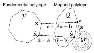
Figure 1: Geometrical view of the relaxed MLD process.

III-B Normal cone

We here review the linear vector channel model again. The received vector $\mbox{\boldmath$r$}\in{\cal R}^{n}$ is given by $\mbox{\boldmath$r$}=A\mbox{\boldmath$x$}+\mbox{\boldmath$b$}+\mbox{\boldmath$z$}$. The transmitted vector $x$ is a (codeword) vertex of a fundamental polytope. The additive noise vector $\mbox{\boldmath$z$}\in{\cal R}^{n}$ is assumed to be generated according to the probability density function $p(\mbox{\boldmath$z$})$.

In order analyze the block error performance of the relaxed ML decoder, a necessary and sufficient condition for the optimal points of the relaxed MLD problem must be established. The normal cone defined below is the essential basis of such a necessary and sufficient condition.

Definition 5 (Normal cone)

Let ${\cal F}\subset{\cal R}^{n}$ be a polytope. Suppose that $\mbox{\boldmath$x$}\in{\cal F}$. The normal cone at $x$ is defined by

$$N_{\cal F}(\mbox{\boldmath$x$})\stackrel{{\scriptstyle\triangle}}{{=}}\{\mbox{\boldmath$y$}\in{\cal R}^{n}:\mbox{\boldmath$y$}^{t}(\mbox{\boldmath$x$}^{\prime}-\mbox{\boldmath$x$})\leq 0,\forall\mbox{\boldmath$x$}^{\prime}\in{\cal F}\}.$$ (18)

The vectors belonging to $N_{\cal F}(\mbox{\boldmath$x$})$ are called the normal vectors of ${\cal F}$ at $x$. ∎

From the definition, it is clear that the normal cone is a closed convex cone including the origin $0^{n}$. If $x$ is included in the interior set of ${\cal F}$, $N_{\cal F}(\mbox{\boldmath$x$})=\{0^{n}\}$ holds because there exists an $\epsilon$-ball ($\epsilon>0$) centered at $x$ which is totally included in ${\cal F}$. We next consider the case where $x$ is on a facet $S$ of ${\cal F}$ and let $z$ be an orthogonal (normal) vector to $S$. It can be verified that $t\mbox{\boldmath$z$}^{t}(\mbox{\boldmath$x$}^{\prime}-\mbox{\boldmath$x$})\leq 0$ holds for any $\mbox{\boldmath$x$}^{\prime}\in{\cal F}$, where $t$ is a non-negative real number. We can show that vectors $t\mbox{\boldmath$z$}$ are the only vectors that satisfy the inequality. This means that $N_{\cal F}(\mbox{\boldmath$x$})=\{t\mbox{\boldmath$z$}:t\geq 0\}$. Finally , we consider the case where $x$ is a vertex of the polytope ${\cal F}$. Suppose that $x$ is given as the intersection of facets $S_{1},S_{2},\ldots S_{k}$. The vectors $\mbox{\boldmath$z$}_{1},\mbox{\boldmath$z$}_{2},\ldots,\mbox{\boldmath$z$}_{k}$ are the normal vectors corresponding to these facets, respectively. In that case, we can show that

$$\mbox{\boldmath$y$}\in\{t_{1}\mbox{\boldmath$z$}_{1}+\cdots t_{k}\mbox{\boldmath$z$}_{k}:t_{1},t_{2},\ldots,t_{k}\geq 0\}$$ (19)

satisfies $\mbox{\boldmath$y$}^{t}(\mbox{\boldmath$x$}^{\prime}-\mbox{\boldmath$x$})\leq 0$ for any $\mbox{\boldmath$x$}^{\prime}\in{\cal F}$ and vice versa. This leads to the following statement:

$$N_{\cal F}(\mbox{\boldmath$x$})=\{t_{1}\mbox{\boldmath$z$}_{1}+\cdots t_{k}\mbox{\boldmath$z$}_{k}:t_{1},t_{2},\ldots,t_{k}\geq 0\}$$ (20)

holds if $x$ is a vertex of ${\cal F}$.

The shifted normal cone $N_{\cal F}(\mbox{\boldmath$x$})+\mbox{\boldmath$x$}$ is defined by

$$N_{\cal F}(\mbox{\boldmath$x$})+\mbox{\boldmath$x$}\stackrel{{\scriptstyle\triangle}}{{=}}\{\mbox{\boldmath$y$}+\mbox{\boldmath$x$}:\mbox{\boldmath$y$}\in N_{\cal F}(\mbox{\boldmath$x$})\},$$ (21)

which is a shifted cone starting from $x$. Figure 2 illustrates the shifted normal cones for a two-dimensional polytope. The black circles denote the point $x$. The figure depicts the three cases discussed above ($x$ is on (1)the interior set, (2)a facet, (3)a vertex).

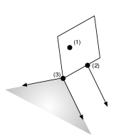
Figure 2: Shifted normal cones.

III-C Optimality condition and decodable noise region

The next lemma is the basis of the proof of the Karush-Kuhn-Tucker condition for convex optimization problems.

Lemma 1 (Condition for global optimum)

Assume that ${\cal F}\subset{\cal R}^{n}$ is a convex set. Let $f(\mbox{\boldmath$x$})$ be a convex function to be minimized subject to the convex constraint $\mbox{\boldmath$x$}\in{\cal F}$. We assume that $f(\mbox{\boldmath$x$})$ is differentiable at any $\mbox{\boldmath$x$}\in{\cal F}$. If and only if

$$-\nabla f(\mbox{\boldmath$x$}^{*})\in N_{\cal F}(\mbox{\boldmath$x$}^{*})$$ (22)

holds, $\mbox{\boldmath$x$}^{*}$ is the global minimum of the convex optimization problem.
(Proof) We omit the proof of this Lemma since it can be found in standard textbooks on non-linear optimization, such as [14]. ∎

This lemma can be used to specify the set of decodable noise using a relaxed ML decoder. For this purpose, it is convenient to introduce the set of decodable noise patterns.

Definition 6 (Decodable noise region)

Let $\mbox{\boldmath$r$}\in{\cal R}^{n}$ be a received vector. For any $\mbox{\boldmath$s$}\in{\cal Q}$, the decodable noise region $D(\mbox{\boldmath$s$})$ corresponding to $s$ is defined by

$$D(\mbox{\boldmath$s$})\stackrel{{\scriptstyle\triangle}}{{=}}\{\mbox{\boldmath$r$}-\mbox{\boldmath$s$}\in{\cal R}^{n}:-\nabla d(\mbox{\boldmath$s$},\mbox{\boldmath$r$})\in N_{\cal Q}(\mbox{\boldmath$s$})\}.$$ (23)

∎

The meaning of the decodable noise region becomes clear in the following corollary:

Corollary 1

Assume that $x$ is a point in the fundamental polytope ${\cal P}$. The received vector $\mbox{\boldmath$r$}=A\mbox{\boldmath$x$}+\mbox{\boldmath$b$}+\mbox{\boldmath$z$}\in{\cal R}^{n}$ can be correctly decoded (i.e., $\mbox{\boldmath$x$}=\hat{\mbox{\boldmath$x$}}$ holds) using the relaxed ML decoder if $\mbox{\boldmath$z$}\in D(A\mbox{\boldmath$x$}+\mbox{\boldmath$b$})$ holds.
(Proof) From the assumption $\mbox{\boldmath$z$}=\mbox{\boldmath$r$}-A\mbox{\boldmath$x$}-\mbox{\boldmath$b$}\in D(A\mbox{\boldmath$x$}+\mbox{\boldmath$b$})$, and so together with the definition of the decodable noise region, we have

$$-\nabla d(A\mbox{\boldmath$x$}+\mbox{\boldmath$b$},\mbox{\boldmath$r$})\in N_{\cal Q}(A\mbox{\boldmath$x$}+\mbox{\boldmath$b$}).$$ (24)

Since the function $d(\cdot,\cdot)$ is convex with respect to the first argument, we can use Lemma 1 to verify that the output from the relaxed ML decoder is $\hat{\mbox{\boldmath$s$}}=A\mbox{\boldmath$x$}+\mbox{\boldmath$b$}$. Applying the inverse affine map, we can obtain the correct estimate:

$$\hat{\mbox{\boldmath$x$}}=A^{-1}(\hat{\mbox{\boldmath$s$}}-\mbox{\boldmath$b$})=\mbox{\boldmath$x$}.$$ (25)

∎

The decodable noise region of $x$ completely characterizes the block error probability when the vector $\mbox{\boldmath$x$}\in{\cal P}$ is sent. We here consider the probability of the event that the estimate $\hat{\mbox{\boldmath$x$}}$ obtained from the relaxed ML decoder coincides with the transmitted codeword vertex $\mbox{\boldmath$x$}\in{\cal P}$. This probability is expressed as expressed as

$$P_{C}(\mbox{\boldmath$x$}) \stackrel{{\scriptstyle\triangle}}{{=}} {\rm Prob}\{\mbox{\boldmath$x$}=\hat{\mbox{\boldmath$x$}}\}$$ (26)

$$= {\rm Prob}\{\mbox{\boldmath$z$}\in D(A\mbox{\boldmath$x$}+\mbox{\boldmath$b$})\}$$ (27)

$$= \int_{D\left(A\mbox{\boldmath$x$}+\mbox{\boldmath$b$}\right)}p(\mbox{\boldmath$z$})dz_{1}dz_{2}\cdots dz_{n},$$ (28)

where $p(\mbox{\boldmath$z$})$ is the probability density function of the additive noise $z$.

The next example considers the case of the Gaussian linear vector channel.

Example 2

Assume that $z_{i}$ is an independent Gaussian random variable with zero mean and variance $\sigma^{2}$, that is, assume that the noise PDF $p(\mbox{\boldmath$z$})$ is given by

$$p(\mbox{\boldmath$z$})=\frac{1}{(2\pi\sigma^{2})^{n/2}}\exp\left(-\sum_{i\in[1,n]}\frac{z_{i}^{2}}{2\sigma^{2}}\right).$$ (29)

For this case, $d(\mbox{\boldmath$s$},\mbox{\boldmath$r$})\stackrel{{\scriptstyle\triangle}}{{=}}||\mbox{\boldmath$r$}-\mbox{\boldmath$s$}||^{2}$ is used as the distance measure for the relaxed ML decoder. It is easy to verify that

$$-\nabla d(\mbox{\boldmath$s$},\mbox{\boldmath$r$})\propto(\mbox{\boldmath$r$}-\mbox{\boldmath$s$})$$ (30)

holds. From this proportional relation, we can obtain the equivalence relation

$$D(\mbox{\boldmath$s$})=N_{\cal Q}(\mbox{\boldmath$s$}).$$ (31)

Suppose that a codeword vertex $\mbox{\boldmath$x$}\in{\cal P}$ is sent and $\mbox{\boldmath$r$}=A\mbox{\boldmath$x$}+\mbox{\boldmath$b$}+\mbox{\boldmath$z$}$ is observed at the receiver side. By using the equivalence relation (31) and substituting for $p(\mbox{\boldmath$z$})$ from equation (29) into equation (28), we have the correct decision probability $P_{C}(\mbox{\boldmath$x$})$ of the relaxed ML decoder for the Gaussian linear vector channel:

$$P_{C}(\mbox{\boldmath$x$})=\frac{1}{(2\pi\sigma^{2})^{n/2}}\int_{N_{\cal Q}(A\mbox{\boldmath$x$}+\mbox{\boldmath$b$})}\exp\left(-\sum_{i\in[1,n]}\frac{z_{i}^{2}}{2\sigma^{2}}\right)d\mbox{\boldmath$z$},$$ (32)

where $d\mbox{\boldmath$z$}\stackrel{{\scriptstyle\triangle}}{{=}}dz_{1}dz_{2}\cdots dz_{n}$. ∎

This example shows that the error performance of the relaxed ML decoder is dominated by the shape of the set of normal cones $N_{\cal Q}(A\mbox{\boldmath$x$}+\mbox{\boldmath$b$})$ where $x$ is a codeword vertex of the fundamental polytope ${\cal P}$.

III-D Analysis for successive decoding

It is highly desirable to perform another decoding process, which is called secondary decoding, after a relaxed MLD process. This is because the relaxed ML decoder may output a non-vertex point as the solution of the minimization problem. If such a non-vertex point is close enough to the transmitted vertex, it can be corrected with a secondary decoding process. Secondary decoding can thus improve the overall decoding performance.

The successive decoding process is given as follows.

$$\hat{\mbox{\boldmath$x$}}_{1} = \arg\min_{\mbox{\boldmath$x$}\in{\cal P}}d(A\mbox{\boldmath$x$}+\mbox{\boldmath$b$},\mbox{\boldmath$r$})$$ (33)

$$\hat{\mbox{\boldmath$x$}}_{2} = \Gamma(\hat{\mbox{\boldmath$x$}}_{1}).$$ (34)

The decoding rule (33) is just the relaxed MLD rule, while the rule (34) corresponds to the secondary decoding. The function $\Gamma:{\cal R}^{n}\rightarrow{\cal R}^{n}$ represents the decoding function for secondary decoding. For example, $\Gamma\stackrel{{\scriptstyle\triangle}}{{=}}(\Gamma_{1},\Gamma_{2},\ldots,\Gamma_{n})$ which is defined by

$$\Gamma_{i}(a_{i})=\left\{\begin{array}[]{cc}0,&a_{i}<0.5\\ 1,&a_{i}\geq 0.5\\ \end{array}\right.$$ (35)

is a possible secondary decoding function. This function quantizes a fractional value in the output vector from the relaxed ML decoder. Another example of the secondary decoding is the built-in min-sum decoder implemented in the interior point decoding presented in the next section.

In the following analysis, the decision region of the secondary decoding plays a crucial role. The decision region of $x$, where $x$ is a codeword vertex of ${\cal P}$, is given by

$$\Delta(\mbox{\boldmath$x$})\stackrel{{\scriptstyle\triangle}}{{=}}\{\mbox{\boldmath$r$}\in{\cal R}^{n}:\mbox{\boldmath$x$}=\Gamma(\mbox{\boldmath$r$})\}.$$ (36)

We assume that $\Delta(\mbox{\boldmath$x$})$ and $\Delta(\mbox{\boldmath$x$}^{\prime})$ are disjoint if $\mbox{\boldmath$x$}\neq\mbox{\boldmath$x$}^{\prime}$. In the following, we assume a Gaussian linear vector channel for simplicity.

Definition 7 (Union of the shifted normal cones)

The union of the shifted normal cones associated with the successive decoding is defined by

$$T(\mbox{\boldmath$x$})\stackrel{{\scriptstyle\triangle}}{{=}}\bigcup_{\mbox{\boldmath$x$}^{\prime}\in\Delta(\mbox{\boldmath$x$})}\left[N_{\cal Q}(A\mbox{\boldmath$x$}^{\prime}+\mbox{\boldmath$b$})+(A\mbox{\boldmath$x$}^{\prime}+\mbox{\boldmath$b$})\right].$$ (37)

The next corollary shows that the set $T(\mbox{\boldmath$x$})$ can be considered to be the decision region corresponding to the transmitted vector $x$.

Corollary 2

Assume that $\mbox{\boldmath$x$}\in{\cal P}$ is a codeword vertex and is sent to the channel. The receiver obtains $\mbox{\boldmath$r$}=A\mbox{\boldmath$x$}+\mbox{\boldmath$b$}+\mbox{\boldmath$z$}$ as the channel output. The successive decoder outputs the correct estimate $\hat{\mbox{\boldmath$x$}}=\mbox{\boldmath$x$}$ if $\mbox{\boldmath$r$}\in T(\mbox{\boldmath$x$})$.
(Proof) The proof is almost same as the proof of Corollary 1, and so is omitted. ∎

Figure 3 illustrates the decision region of the successive decoding. We can see that $T(\mbox{\boldmath$x$})$ totally includes the shifted normal cone of $x$. This means that secondary decoding can improve the correct decision probability $P_{C}(\mbox{\boldmath$x$})$ in the case of Gaussian linear vector channels.

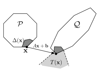
Figure 3: Decision region of the successive decoding.

Due to Corollary 2, error analysis of the successive decoding can be divided into several sub-problems: (i) analysis of the local structure of the fundamental polytope, (ii) analysis of the the decision region $\Delta(\mbox{\boldmath$x$})$ and (iii) numerical evaluation of the error probability (via multi-dimensional integration or bounds). Of course, these sub-problems are not easy to solve for long binary linear codes. However, the geometrical perspective established in this section will become a solid basis of further error analysis and it helps us to understand the behavior of a sub-optimal relaxed ML decoder.

IV Overview of Interior Point Decoding

Although the relaxed MLD problem is easier to solve than the original MLD problem, it is still a computationally difficult problem and we must consider techniques to solve it efficiently. Since the relaxed MLD problem can be seen as a convex optimization problem, it is reasonable to apply conventional optimization techniques to this problem. In this section, the interior point decoding algorithm for linear vector channels will be presented. The proposed decoding algorithm is based on the idea of the interior point algorithm for convex optimization [4].

In this section, we first briefly review the idea of the interior point algorithm based on a barrier function method, before describing the overall structure of the proposed decoding algorithm.

The details of the sub-procedures required for the algorithm are explained in the subsequent subsections.

IV-A Barrier function method: a brief review

The interior point algorithm describes a class of optimization algorithms for solving LP and convex optimization problems. Many sophisticated interior point algorithms have been developed [4], here we explain the simplest algorithm which is based on a barrier function method.

Let $f(\mbox{\boldmath$x$})(\mbox{\boldmath$x$}\in{\cal R}^{n})$ be a real-valued function to be minimized. Assume that $f(\mbox{\boldmath$x$})$ is a convex function and the feasible region ${\cal F}$ is a convex subset of ${\cal R}^{n}$. A convex optimization problem is a minimization problem with a constraint of the form

$$\mbox{minimize }f(\mbox{\boldmath$x$}),\mbox{ s.t. }\mbox{\boldmath$x$}\in{\cal F}.$$ (38)

The key idea of the barrier function method is to convert the original convex optimization problem (38) into an unconstrained optimization problem by using a barrier function. Let $B(\mbox{\boldmath$x$})$ be a barrier function which has the following properties: (i) $B(\mbox{\boldmath$x$})$ takes a finite real value if $\mbox{\boldmath$x$}\in{\cal F}^{*}$ where ${\cal F}^{*}$ is the interior set of the feasible region ${\cal F}$; (ii) $B(\mbox{\boldmath$x$})=\infty$ if $\mbox{\boldmath$x$}\notin{\cal F}^{*}$; (iii) $B(\mbox{\boldmath$x$})$ is differentiable and convex. Combining the original objective function $f(\mbox{\boldmath$x$})$ with the barrier function $B(\mbox{\boldmath$x$})$, we have a new convex objective function which is called a merit function $\psi(\mbox{\boldmath$x$})\stackrel{{\scriptstyle\triangle}}{{=}}tf(\mbox{\boldmath$x$})+B(\mbox{\boldmath$x$}).$ The parameter $t$ is a positive real number called a scale parameter.

Thus the barrier function method replaces the original problem (38) by the optimization problem

$$\mbox{minimize }\psi(\mbox{\boldmath$x$}),\mbox{ s.t. }\mbox{\boldmath$x$}\in{\cal R}^{n}.$$ (39)

It is observed that the constraints in (38) are absorbed into the barrier function and thus problem (39) is an unconstrained minimization problem for a convex function $\psi(\mbox{\boldmath$x$})$. In order to solve this problem, we can therefore exploit an efficient numerical optimization algorithm such as the gradient descent method or the Newton method.

Of course, the unconstrained problem (39) and the original problem (38) are not Identical, and the optimal point $\mbox{\boldmath$x$}_{1}^{*}$ of problem (38) will not, in general, coincide with the optimal point $\mbox{\boldmath$x$}_{2}^{*}$ of (39). However, when $t\rightarrow\infty$, we can expect that $\mbox{\boldmath$x$}_{2}^{*}\rightarrow\mbox{\boldmath$x$}_{1}^{*}$ because the effect from the barrier function becomes relatively small in this limit. On the other hand, smaller values of $t$ improve the rate of convergence of the solution. As $t$ becomes larger, the barrier function approaches a discontinuous function, which in general tends to retard the rate of convergence.

A well-known recipe to obtain a point $\mbox{\boldmath$x$}_{2}^{*}$ close to $\mbox{\boldmath$x$}_{1}^{*}$ is to perform the gradient descent or the Newton method several times while $t$ is gradually increased. The interior point algorithm based on the barrier function method consists of the two loops called inner and outer loops, respectively (see Fig.4 left). In the inner loop, $\psi(\mbox{\boldmath$x$})$ is minimized using the gradient descent or the Newton method. The aim of the outer loop is that of a scaling of $t$. In each iteration of the outer loop, $t$ is multiplied by a positive constant $\alpha$, and so the value of $t$ increases as the number of outer iterations increases.

The name ”interior point” comes from the fact that search points (the tentative candidates for the optimal point) located on a trajectory moving towards the optimal point are always contained in ${\cal F}^{*}$ (see Fig.4 right). For faster convergence, it is hoped that the trajectory of the search points does not approach the boundary of the feasible region. The barrier function is introduced to prevent a search point from approaching the boundary.

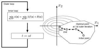
Figure 4: Interior point algorithm based on the barrier function method.

IV-B Objective and merit functions for interior point decoding

We here apply the interior point algorithm based on the barrier function method to the relaxed MLD problem (13). In the following, we will assume a Gaussian linear vector channel for simplicity, but the extension to the non-Gaussian (or correlated Gaussian) case is straightforward. The objective function to be minimized is, therefore, $||\mbox{\boldmath$r$}-(A\mbox{\boldmath$x$}+\mbox{\boldmath$b$})||^{2}$.

Definition 8 (Objective function)

The objective function $f(\mbox{\boldmath$x$})(\mbox{\boldmath$x$}\in{\cal R}^{n})$ for the relaxed MLD problem is defined by

$$f(\mbox{\boldmath$x$}) \stackrel{{\scriptstyle\triangle}}{{=}} ||\mbox{\boldmath$r$}-(A\mbox{\boldmath$x$}+\mbox{\boldmath$b$})||^{2}$$ (40)

$$= \sum_{i\in[1,n]}\left(r_{i}-\left(\sum_{j\in[1,n]}a_{ij}x_{j}+b_{i}\right)\right)^{2},$$

where $r_{i}$ and $b_{i}$ are $i$th elements of $r$ and $b$, respectively. The symbol $a_{ij}$ denotes the $(i,j)$-element of the interference matrix $A$. ∎

The function $f(\mbox{\boldmath$x$})$ is a differentiable, convex function, with these properties making it suitable for use in the the gradient descent and Newton methods. In the case of non-Gaussian linear vector channels, we can also define an appropriate objective function.

Various choices exist for the form of the barrier function. In this paper, we adopt $b(x)\stackrel{{\scriptstyle\triangle}}{{=}}-\ln(-x)$ as the basis of the barrier function, which is called a log-barrier function. It is clear that $b(x)=\infty$ holds when $x=0$; on the other hand, $b(x)$ takes a finite value if $x<0$. Furthermore, $b(x)$ is a convex function. Thus the function $b(x)$ satisfies the requirements of the barrier functions as discussed above. Moreover, the derivative of $b(x)$, namely,

$$\frac{d}{dx}b(x)=-\frac{1}{x}$$ (41)

is simple enough for implementation in a decoding algorithm. The log-barrier function including the parity constraints and box constraints is given below.

Definition 9 (Log-barrier function)

The log-barrier function for the fundamental polytope $B(\mbox{\boldmath$x$})(\mbox{\boldmath$x$}\in{\cal R}^{n})$ is defined by

$$B(\mbox{\boldmath$x$}) \stackrel{{\scriptstyle\triangle}}{{=}} -\sum_{i\in[1,m]}\sum_{S\subset T_{i}}\ln\left[-\left(1+\sum_{t\in S}(x_{t}-1)-\sum_{t\in A_{i}\backslash S}x_{t}\right)\right]$$ (42)

$$- \sum_{j\in[1,n]}\ln\left[-(-x_{j})\right]-\sum_{j\in[1,n]}\ln\left[-(x_{j}-1)\right].$$

∎

The log-barrier function $B(\mbox{\boldmath$x$})$ inherits the properties of $b(x)$; $B(\mbox{\boldmath$x$})$ is a convex and differentiable function. Furthermore, if $\mbox{\boldmath$x$}\notin{\cal P^{*}}$, then $B(\mbox{\boldmath$x$})=\infty$ holds; otherwise $B(\mbox{\boldmath$x$})<\infty$.

The definition of the merit function including both the objective function and the log-barrier function is as follows.

Definition 10 (Merit function)

For any $\mbox{\boldmath$x$}\in{\cal R}^{n}$, the merit function $\psi^{(t)}(\mbox{\boldmath$x$})$ for the relaxed ML decoding problem is given by

$$\psi^{(t)}(\mbox{\boldmath$x$})\stackrel{{\scriptstyle\triangle}}{{=}}tf(\mbox{\boldmath$x$})+B(\mbox{\boldmath$x$}),$$ (43)

where $t$ is a positive real number. ∎

The first term of $\psi^{(t)}(\mbox{\boldmath$x$})$ is a scaled version of the objective function. The second term is the log-barrier function corresponding to the fundamental polytope. Since the sum of convex functions is also a convex function, $\psi^{(t)}(\mbox{\boldmath$x$})$ is a convex function. Note that $\psi^{(t)}(\mbox{\boldmath$x$})$ takes a finite value if $\mbox{\boldmath$x$}\in{\cal P}^{*}$.

IV-C Partial Response Channels

In the field of magnetic recording, the PR channel model is often exploited as a basis of system design. Interferences arising from neighboring symbols are linearly superimposed on the current symbol, with these interferences increasing the complexity of the decoding process.

Let $\delta+1$-real numbers $\{h_{0},h_{1},\ldots,h_{\delta}\}$ be the partial response (PR) coefficients. The parameter $\delta$ is called the degree of the PR channel. The PR channel can be regarded as a discrete time finite impulse response (FIR) filtered channel with additive white Gaussian noises (see Fig.5). The definition of PR channel is given below.

Definition 11 (Partial response channel)

A binary vector $\mbox{\boldmath$x$}=(x_{1},x_{2},\ldots,x_{n})\in C$ is transmitted to the channel defined by

$$r_{j}=\sum_{d=0}^{\delta}h_{d}(1-2x_{j-d})+z_{j},\quad j\in[1,n],$$ (44)

where $z_{j}(j\in[1,n])$ is an independent Gaussian random variable with mean 0 and variance $\sigma^{2}$. By convention, we assume that

$$x_{-(\delta-1)}=x_{-(\delta-2)}=\cdots=x_{-1}=x_{0}=\frac{1}{2},$$ (45)

which simplifies the treatment of the boundary condition. The channel is called a PR channel. The signal to noise ratio ( $snr$ ) of the PR channel is defined by

$$snr\stackrel{{\scriptstyle\triangle}}{{=}}\left(\sum_{d=0}^{\delta}h_{d}^{2}\right)/\sigma^{2}.$$ (46)

∎

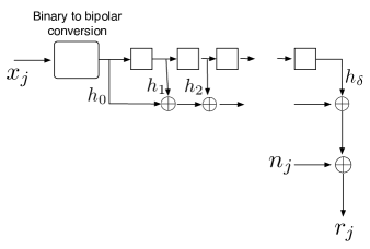
Figure 5: Block diagram of partial response channels.

As shown in Fig.5, the $j$th received symbol $r_{j}$ consists of the weighted sum of $\{1-2x_{j},1-2x_{j-1},\ldots,1-2x_{j-\delta}\}$ and the noise term. It is clear that the PR channel can be expressed in the following linear vector channel form:

$$\mbox{\boldmath$r$}=A\mbox{\boldmath$x$}+\mbox{\boldmath$b$}+\mbox{\boldmath$z$},$$ (47)

where $A$ and $b$ are given by

$$A=-2\left(\begin{array}[]{cccc}h_{0}&\cdots&&\\ h_{1}&h_{0}&\cdots&\\ \vdots&\vdots&\vdots&\vdots\\ h_{\delta}&\cdots&h_{0}&\cdots\\ \vdots&\vdots&\vdots&\vdots\\ \cdots&h_{\delta}&\cdots&h_{0}\end{array}\right),\mbox{\boldmath$b$}=\left(\begin{array}[]{c}h_{0}\\ h_{1}+h_{0}\\ \vdots\\ \sum_{d=0}^{\delta-1}h_{d}\\ \sum_{d=0}^{\delta}h_{d}\\ \vdots\\ \sum_{d=0}^{\delta}h_{d}\\ \end{array}\right).$$ (48)

The PR channels can be regarded as linear vector channels with a sparse interference matrix $A$. Thus, the PR channel is an ideal candidate for the interior point decoding. Throughout the paper, this channel will be used as an example of a Gaussian linear vector channel.

For PR channels, the objective function $f(\mbox{\boldmath$x$})$ takes the following form:

$$f(\mbox{\boldmath$x$})=\sum_{j=1}^{n}\left(r_{j}-\left(\sum_{d=0}^{\delta}h_{d}(1-2x_{j-d})\right)\right)^{2}.$$ (49)

The partial derivative of $tf(\mbox{\boldmath$x$})$ with respect to a variable $x_{p}(p\in[1,n])$ is required to compute the approximate gradient presented later. From the objective function (49), we immediately have

$$\frac{\partial}{\partial x_{p}}tf(\mbox{\boldmath$x$}) = t\sum_{j=1}^{n}\frac{\partial}{\partial x_{p}}\left(r_{j}-\sum_{d=0}^{\delta}h_{d}(1-2x_{j-d})\right)^{2}$$ (50)

$$= 4t\sum_{j=k}^{p+\delta}h_{j-p}\left(r_{j}-\sum_{d=0}^{\delta}h_{d}(1-2x_{j-d})\right).$$

It can be observed that the number of additions required to evaluate equation (50) is proportional to $\delta^{2}$. This means that evaluation of the gradient $\nabla tf(\mbox{\boldmath$x$})$ takes $O(n)$ computational time if $\delta$ is constant.

We next consider the Hessian of the objective function, which is required for the Newton method to be discussed later. From (50), we have

$$\frac{\partial}{\partial x_{p}}tf(\mbox{\boldmath$x$}) = 4t\sum_{j=p}^{p+\delta}h_{j-p}\left(r_{j}-\sum_{d=0}^{\delta}h_{d}(1-2x_{j-d})\right)$$ (51)

$$= 8t\sum_{j=p}^{p+\delta}\sum_{d=0}^{\delta}h_{j-p}h_{d}x_{j-d}+K$$

for $p\in[1,n]$. The symbol $K$ denotes terms that do not contain $x_{k}$. Let $q\stackrel{{\scriptstyle\triangle}}{{=}}j-d$. The second derivative of the objective function is given by

$$\frac{\partial}{\partial x_{p}x_{q}}tf(\mbox{\boldmath$x$}) = 8t\sum_{j=p}^{p+\delta}h_{j-p}h_{j-q}I[j-q\in[0,\delta]].$$ (52)

By setting $j-p=a$, we obtain the following expression:

$$\frac{\partial}{\partial x_{p}x_{q}}tf(\mbox{\boldmath$x$}) = 8t\sum_{a=0}^{\delta}h_{a}h_{a+p-q}I[a+p-q\in[0,\delta]]$$ (53)

for $p\in[1,n]$, $q\in[1,n]$.

IV-D Overall structure of interior point decoding

The goal of the interior point decoding is to solve the relaxed MLD problem by using an interior point algorithm based on the barrier function method. The interior point decoding consists of two nested loops: an outer loop and an inner loop. The inner loop corresponds to either an approximate gradient descent method or an approximate Newton method, both of which try to minimize the merit function $\psi^{(t)}(\mbox{\boldmath$x$})$. The outer loop contains the following sub-procedures: inner loop, built-in min-sum decoding, and scaling of the parameter $t$. The details of these sub-procedures are discussed in the following subsections.

The procedure $InteriorPoint(\cdot)$ is the main procedure for the interior point decoding. The positive integer parameters $O_{max}$ and $I_{max}$ specify the number of iterations executed in the outer and inner loops, respectively. The parameter $t_{0}$ is the initial scale parameter, which is a positive real number.

Procedure: $\hat{\mbox{\boldmath$b$}}:=InteriorPoint(\mbox{\boldmath$r$})$ Input: $\mbox{\boldmath$r$}\in{\cal R}^{n}$ : received word Output: $\hat{\mbox{\boldmath$b$}}\in F_{2}^{n}\bigcup\{*\}$: estimation word Step 1 Let $\mbox{\boldmath$x$}:=(1/2,1/2,\ldots,1/2)$ and $t:=t_{0}$. Step 2 Repeat the following sub-steps (2.1–2.4) $O_{max}$ times: Step 2.1 Repeat the following process $I_{max}$ times: $$\mbox{\boldmath$x$}:=InnerLoop(\mbox{\boldmath$x$},t).$$ Step 2.2 Execute $(p,\hat{\mbox{\boldmath$b$}}):=MinSum(\mbox{\boldmath$x$})$. Step 2.3 If $p=0$, then exit. Step 2.4 Let $t:=\alpha t$. Step 3 Let $\hat{\mbox{\boldmath$b$}}:=*$ ($*$ denotes decoding failure) and then exit.

The heart of the decoding algorithm is the process called $InnerLoop(\cdot)$. This procedure updates a search point $x$ using the gradient descent method or the Newton method so as to minimize the merit function $\psi^{(t)}(\mbox{\boldmath$x$})$. Since the search point $x$ must always be contained in ${\cal P}^{*}$, we need to check the feasibility of the search point in this process.

After the execution of the inner loop, built-in min-sum decoding is performed to obtain an estimate of the transmitted word. The role of the min-sum decoding is to find a codeword near to the current search point obtained from the inner loop process.

In the interior point method, a search point must lie in the feasible region ${\cal P}^{*}$ in all iterations of the procedure. The following lemma justifies the choice of $\mbox{\boldmath$x$}=(1/2,1/2,\ldots,1/2)$ as the initial search point.

Lemma 2

If $H$ is a row-regular parity check matrix with $w_{r}\geq 3$, then the initial search point $\mbox{\boldmath$x$}=(1/2,1/2,\ldots,1/2)$ is a feasible point, i.e., $\mbox{\boldmath$x$}\in{\cal P}^{*}$.
(Proof) It is evident that $x$ satisfies the box constraints. Thus, we only need to consider the parity constraints. For any $i\in[1,m],S\in T_{i}$, we have

$$1+\sum_{t\in S}\left(\frac{1}{2}-1\right)-\sum_{t\in A_{i}\backslash S}\frac{1}{2}=1-\frac{1}{2}|A_{i}|=1-\frac{1}{2}w_{r}<0$$ (54)

using the assumption $w_{r}\geq 3$ and row-regularity. This means that $x$ also satisfies the parity constraints. ∎

IV-E Built-in min-sum decoding

The advantage of exploiting the built-in min-sum decoding process after the inner loop process is the consequent reduction in the required number of outer and inner iterations. If the current search point approaches close enough to a codeword vertex, the built-in decoding process can output the corresponding codeword as an estimate vector. In particular, we need not wait for the search point to converge to a codeword vertex, which in general requires a much longer computational time. Furthermore, the built-in min-sum decoding acts as the secondary decoding discussed in the previous section. That is, it can compensate a non-vertex point obtained from an inner-loop process. Therefore, this built-in decoding process is indispensable for the interior point decoding technique.

In the following, a brief description on the built-in min-sum decoding is given. Let $B_{j}(j\in[1,n])$ be the set of row indices such that $B_{j}\stackrel{{\scriptstyle\triangle}}{{=}}\{i\in[1,m]:h_{ij}=1\}.$ The following procedure $MinSum(\mbox{\boldmath$x$})$ is the standard log-domain min-sum algorithm with a dumping factor (also known as normalized min-sum algorithm [13]).

Procedure: $(p,\hat{\mbox{\boldmath$b$}}):=MinSum(\mbox{\boldmath$x$})$ Input: $\mbox{\boldmath$x$}\in{\cal P}^{*}$: current search point Output: $(p,\hat{\mbox{\boldmath$b$}})$: parity flag $p$ and tentative estimate vector $\hat{\mbox{\boldmath$b$}}$ Step 1 Compute the log likelihood ratios: $$\lambda_{j}:=\ln\left(\frac{1-x_{j}}{x_{j}}\right)$$ (55) for $j\in[1,n]$. Set $\xi_{i\rightarrow j}:=0$ for all pair $(i,j)$ satisfying $j\in A_{i}$. Step 2 Repeat the following sub-steps (2.1–2.4) $L_{max}$ times. Step 2.1 For all pairs $(i,j)$ satisfying $j\in A_{i}$, evaluate $$\eta_{j\rightarrow i}:=\lambda_{j}+\sum_{k\in B_{j}\backslash i}\xi_{k\rightarrow j}.$$ (56) Step 2.2 For all pairs $(i,j)$ satisfying $j\in A_{i}$, evaluate $\displaystyle\xi_{i\rightarrow j}$ $\displaystyle:=$ $\displaystyle\kappa\left(\prod_{k\in A_{i}\backslash j}\mbox{sign}(\eta_{k\rightarrow i})\right)$ (57) $\displaystyle\times$ $\displaystyle\min_{k\in A_{i}\backslash j}|\eta_{k\rightarrow i}|.$ The function $\mbox{sign}(\cdot)$ is defined by $$\mbox{sign}(x)=\left\{\begin{array}[]{cc}1,&x\geq 0\\ -1&x<0.\\ \end{array}\right.$$ (58) Step 2.3 For $j\in[1,n]$, decide the tentative estimate word $\hat{\mbox{\boldmath$b$}}=(\hat{b}_{1},\hat{b}_{2},\ldots,\hat{b}_{n})$ in the following way: $$\hat{b}_{j}:=\left\{\begin{array}[]{cc}0,&\lambda_{j}+\sum_{k\in B_{j}}\xi_{k\rightarrow j}\geq 0\\ 1,&\lambda_{j}+\sum_{k\in B_{j}}\xi_{k\rightarrow j}<0.\\ \end{array}\right.$$ (59) Step 2.4 If $H\hat{\mbox{\boldmath$b$}}=\mbox{\boldmath$0$}$ holds, then let $p:=0$ and exit. Step 3 Let $p:=1$.

In the initialization part, the LLRs used in the min-sum decoding are computed as expression (55). Since $0<x_{j}<1$ holds for any $j\in[1,n]$, we here regard $x_{j}$ as the probability such that the $j$th transmitted symbol is 1. The constant $\kappa$ which appears in expression (57) is the dumping factor $(\kappa\simeq 0.7$–$0.9)$ which improves decoding performance of the min-sum decoding.

V Inner loop based on gradient descent method

The gradient descent method is a well-known minimization method for an unconstrained convex function with a known first derivative. The convergence of the gradient descent method is relatively slow compared with methods that utilize second derivatives (i.e., the Hessian) of the objective function, such as the Newton method, but the gradient descent method is much easier to implement.

V-A Brief review on gradient descent method

We here briefly review the gradient descent method. Let $h(\mbox{\boldmath$x$}),\mbox{\boldmath$x$}\in{\cal R}^{n}$ be a real-valued convex function to be minimized. In the process of the gradient descent method, a search point gradually approaches the optimal point. For each iteration of the minimization process, the search point $x$ is updated as

$$\mbox{\boldmath$x$}:=\mbox{\boldmath$x$}-s\nabla h(\mbox{\boldmath$x$}),$$ (60)

where $\nabla h(\mbox{\boldmath$x$})$ is the gradient of $h(\mbox{\boldmath$x$})$. That is, the search point moves in the descent direction $-\nabla h(\mbox{\boldmath$x$})$. A positive real parameter $s$ is called the step size parameter.

The optimal choice of $s$, for a given $x$, is obtained by solving the following one-dimensional optimization problem:

$$s=\arg\min_{s^{\prime}>0}h(\mbox{\boldmath$x$}-s^{\prime}\nabla h(\mbox{\boldmath$x$})).$$ (61)

This one-dimensional optimization process is usually called the exact line search. Other than the exact line search (61), some inexact line search methods such as the bisection scheme with backtracking [4] also exist. For the exact line search and some of the inexact line searches, it can be proved that the search point eventually converges to the optimal point [4] using the gradient descent update (60).

V-B Approximate gradient descent method

The procedure $InnerLoop(\cdot)$ returns a new search point which is computed from the current search point. In order to make the interior point decoding computationally tractable, some approximations are introduced.

The aim of the procedure $InnerLoop(\cdot)$ is to find the minimum of $\psi^{(t)}(\mbox{\boldmath$x$})$ using a gradient descent method. It uses the approximate gradient (instead of the true gradient $\nabla\psi^{(t)}(\mbox{\boldmath$x$})$) and an inexact line search scheme inside. Thus, strictly speaking, the procedure is an approximation of the gradient descent method.

The following procedure is the main part of the inner loop, which can be regarded as an inexact line search method based on the bisection scheme.

Procedure: $\mbox{\boldmath$x$}:=InnerLoop(\mbox{\boldmath$x$},t)$ Input: $\mbox{\boldmath$x$}\in{\cal P}^{*}$: current search point Output: $x$: updated search point Step 1 Set $s:=1$. Step 2 $\mbox{\boldmath$g$}:=ApproxGradient(\mbox{\boldmath$x$},t)$. Step 3 Let $\tilde{\mbox{\boldmath$x$}}:=\mbox{\boldmath$x$}-s\mbox{\boldmath$g$}$ Step 4 If $IsFeasible(\tilde{\mbox{\boldmath$x$}})=0$, namely $\tilde{\mbox{\boldmath$x$}}\notin{\cal P}^{*}$ holds, then let $s:=s/2$ and return to Step 3. Step 5 Let $\mbox{\boldmath$x$}:=\tilde{\mbox{\boldmath$x$}}$.

Since the vector $x$ is an interior point of the fundamental polytope, there exits $s>0$ satisfying $\mbox{\boldmath$x$}-s\mbox{\boldmath$g$}\in{\cal P}^{*}$. This means that the loop composed of Step 3 and Step 4 must eventually stop.

The process $InnerLoop(\cdot)$ includes the feasibility check in its procedure. Thus, it is guaranteed that the updated point is located in the feasible region ${\cal P}^{*}$. Figure 6 presents an example of a search step of $InnerLoop(\cdot)$. A search process is performed to find a feasible point on the half line starting from the current search point in the opposite direction to that of the approximate gradient vector. For the case shown in Fig.6, the first temporary search point $\tilde{\mbox{\boldmath$x$}}$ is not in ${\cal P}^{*}$. Thus, the step size parameter $s$ is reduced to $s:=s/2$ to produce the second temporary search point, which is a feasible point. As a result, the second point becomes the next search point (i.e., the updated search point).

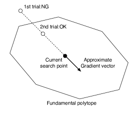
Figure 6: A search step of $InnerLoop(\cdot)$.

The procedure uses the approximate gradient $g$ and does not include an evaluation of the merit function $\psi^{(t)}(\mbox{\boldmath$x$})$. Moreover, only a feasibility check is carried out in the procedure. Thus, we cannot expect the objective function to be a non-increasing function of the number of iterations in this case. This implies that the search point may not converge to the optimal point. However, due to this compromise, we obtain a huge reduction in computational costs. For example, the evaluation of the objective function, which requires a time computational complexity $O(2^{w_{r}}n)$, can be avoided in this procedure. In this paper, we assume that $m$ scales proportional to $n$, namely $m=(1-R)n$, $0<R<1$. In contrast, the execution of the feasibility check and evaluation of the approximate gradient take only $O(w_{r}n)$ computation time. Note that the evaluation of the true gradient of the barrier function $\nabla B(\mbox{\boldmath$x$})$ requires $O(2^{w_{r}}n)$ computation time.

V-C Feasibility check

The purpose of the procedure $IsFeasible(\cdot)$ is to decide the feasibility of a given $\mbox{\boldmath$x$}\in{\cal R}^{n}$. In the interior point method, a search point must lie in the feasible region in all iterations. Thus, the feasibility check is one of the key procedures of the inner loop.

The procedure $IsFeasible(\mbox{\boldmath$x$})$ returns 1 if $\mbox{\boldmath$x$}\in{\cal P}^{*}$; otherwise it returns 0. Of course, we could evaluate all the inequalities (11) and (12) to decide the feasibility of given $x$. However, such a brute-force approach takes $O(2^{w_{r}}n)$ computation time to check the feasibility because the number of inequalities (11) is $2^{w_{r}-1}m$. However, we can do much better as shown in the next lemma and the algorithm.

Lemma 3 (Feasiblity check)

The point $(x_{1},x_{2},\ldots,x_{n})\in{\cal R}^{n}$ belongs to ${\cal P}^{*}$ if and only if $\theta_{i}<0$ for any $i\in[1,m]$ and $0<x_{j}<1$ for any $j\in[1,n]$ where $\theta_{i}(i\in[1,m])$ is defined by

$$\theta_{i}\stackrel{{\scriptstyle\triangle}}{{=}}\max_{S\subset T_{i}}\left[1+\sum_{l\in S}(x_{l}-1)-\sum_{l\in A_{i}\backslash S}x_{l}\right].$$ (62)

(Proof) If $\theta_{i}<0$ for any $i\in[1,m]$ and $0<x_{j}<1$ for any $j\in[1,n]$, then

$$1+\sum_{l\in S}(x_{l}-1)-\sum_{l\in A_{i}\backslash S}x_{l}<0$$ (63)

holds for any $i\in[1,m]$ and $S\subset T_{i}$, because $\theta_{i}$ is the maximum value of $1+\sum_{l\in S}(x_{l}-1)-\sum_{l\in A_{i}\backslash S}x_{l}$. This implies that $x$ is a feasible point.

We then consider the opposite direction. Assume that $\mbox{\boldmath$x$}\notin{\cal P}^{*}$. This means that some of the parity constraints or the box constraints are violated. If some of the box constraints are not satisfied, then there exists $j^{*}\in[1,n]$ such that $x_{j^{*}}$ is not in the open interval between $0$ and $1$. If some of the parity constraints are not satisfied, there exists an index $i^{*}\in[1,m]$ and $S^{*}\subset T_{i^{*}}$ such that

$$1+\sum_{l\in S^{*}}(x_{l}-1)-\sum_{l\in A_{i^{*}}\backslash S^{*}}x_{l}\geq 0.$$ (64)

From the definition of $\theta_{i}$, it is evident that $\theta_{i^{*}}\geq 0$ in such a case. This completes the proof. ∎

Lemma 3 is useful to reduce the computational time required to carry out the feasibility check, because the computational time required to evaluate all $\theta_{i}(i\in[1,m])$ is proportional to $w_{r}m$. In other words, $\theta_{i}$ can be computed without generating all the subsets of odd size in $T_{i}$. We can use an idea similar to maximum likelihood decoding for even weight codes. The following procedure includes such an idea for an efficient computation of $\theta_{i}$.

Procedure: $f:=IsFeasible(\mbox{\boldmath$x$})$ Input: $\mbox{\boldmath$x$}=(x_{1},x_{2},\ldots,x_{n})\in{\cal R}^{n}$: current search point Output: $f$: If $\mbox{\boldmath$x$}\in{\cal P}^{*},$then $f:=1$; otherwise $f:=0$. Step 1 If there exists $j\in[1,n]$ such that $x_{j}$ do not satisfy $0<x_{j}<1$, set $f:=0$ and exit. Step 2 Repeat sub-steps (2.1–2.3) from $i:=1$ to $m$. Step 2.1 For $l\in A_{i}$, set $\displaystyle\beta_{l}^{(i)}$ $\displaystyle:=$ $\displaystyle\left\{\begin{array}[]{cc}0,&x_{l}-1\leq-x_{l}\\ 1,&x_{l}-1>-x_{l}\\ \end{array}\right.$ (67) and evaluate $$u:=1+\sum_{l\in A_{i}}\max\{x_{l}-1,-x_{l}\},$$ (68) and $v:=\sum_{l\in A_{i}}\beta_{l}^{(i)}.$ Step 2.2 If $v$ is even, then update $u$ as $u:=u-\min_{l\in A_{i}}|2x_{l}-1|$ and let $\beta_{l_{min}}^{(i)}:=\beta_{l_{min}}^{(i)}\oplus 1,$ where $l_{min}:=\arg\min_{l\in A_{i}}|2x_{l}-1|.$ Step 2.3 If $u\geq 0$, then set $f:=0$ and exit. Step 3 Set $f:=1$ and exit.

The symbol $\oplus$ denotes addition over $F_{2}$. Let us consider the states of the variables after an execution of the above procedure. Let $S^{\prime}\stackrel{{\scriptstyle\triangle}}{{=}}\{l\in A_{i}:\beta^{(i)}_{l}=1\}$. Suppose the case where $v$ is odd. From this assumption, it is evident that $|S^{\prime}|$ is odd. The right-hand side of (68) can be rewritten as

$$u = 1+\sum_{l\in A_{i}}\max\{x_{l}-1,-x_{l}\}$$ (69)

$$= 1+\sum_{l\in S^{\prime}}(x_{l}-1)-\sum_{l\in A_{i}\backslash S^{\prime}}x_{l}$$

$$= 1+\max_{S\subset T_{i}}\left[\sum_{l\in S}(x_{l}-1)-\sum_{l\in A_{i}\backslash S}x_{l}\right]$$

$$= \theta_{i}.$$

Thus, in this case, $u=\theta_{i}$ holds. We then consider the case where $v$ is even. In such a case, one of the components in $\{\beta_{l}^{(i)}\}_{l\in A_{i}}$ should be flipped so as to make the weight of the binary vector $\{\beta_{l}^{(i)}\}_{l\in A_{i}}$ odd. Let $l^{\prime}$ denote the index at which the bit flip occurs, namely $\beta_{l^{\prime}}^{(i)}:=\beta_{l^{\prime}}^{(i)}\oplus 1$. The bit flipping decreases the value of $u$ to $u-|x_{l}-1-(-x_{l})|=u-|2x_{l}-1|$. Since the aim of the bit flipping is to find the optimal subset with odd size, it is reasonable to determine the index $\l^{\prime}$ according to the values of $|2x_{l}-1|$. Namely, $t_{min}:=\arg\min_{l\in A_{i}}|2x_{l}-1|$ gives the smallest decrement (i.e., the largest value of $u$). Therefore, $u=\theta_{i}$ also holds for this case.

V-D Approximate gradient

The gradient of $\psi^{(t)}(\mbox{\boldmath$x$})$, which is defined on ${\cal P}^{*}$, is given by

$$\nabla\psi^{(t)}(\mbox{\boldmath$x$})\stackrel{{\scriptstyle\triangle}}{{=}}\left(\frac{\partial}{\partial x_{1}}\psi^{(t)}(\mbox{\boldmath$x$}),\frac{\partial}{\partial x_{2}}\psi^{(t)}(\mbox{\boldmath$x$}),\ldots,\frac{\partial}{\partial x_{n}}\psi^{(t)}(\mbox{\boldmath$x$})\right).$$ (70)

We have, after some manipulation, the partial derivative of $\psi^{(t)}(\mbox{\boldmath$x$})$ with respect to the variable $x_{k}(k\in[1,n])$:

$$\frac{\partial}{\partial x_{k}}\psi^{(t)}(\mbox{\boldmath$x$}) = t\frac{\partial}{\partial x_{k}}f(\mbox{\boldmath$x$})+\frac{\partial}{\partial x_{k}}B(\mbox{\boldmath$x$})$$ (71)

$$= t\frac{\partial}{\partial x_{k}}f(\mbox{\boldmath$x$})+\sum_{i\in[1,m]}\sum_{S\subset T_{i}}\tau_{k}^{(i,S)}(\mbox{\boldmath$x$})$$

$$- \frac{1}{x_{k}}-\frac{1}{x_{k}-1},$$

where

$$\tau_{k}^{(i,S)}(\mbox{\boldmath$x$})\stackrel{{\scriptstyle\triangle}}{{=}}\frac{I[k\in A_{i}\backslash S]-I[k\in S]}{1+\sum_{l\in S}(x_{l}-1)-\sum_{l\in A_{i}\backslash S}x_{l}}$$ (72)

for $i\in[1,m]$, $S\subset[1,n]$. The notation $I[condition]$ is the indicator function such that $I[condition]=1$ if $condition$ is true; otherwise, it gives 0. Note that the derivative of the objective function (40) is given by

$$t\frac{\partial}{\partial x_{k}}f(\mbox{\boldmath$x$})=-t\sum_{i\in[1,\ell]}2a_{ik}\left(r_{i}-\left(b_{i}+\sum_{j\in[1,n]}a_{ij}x_{j}\right)\right).$$ (73)

The next example presents the gradient of the merit function of PR channels.

Example 3

For the case of PR channels, we have the following derivative of the merit function:

$$\frac{\partial}{\partial x_{k}}\psi^{(t)}(\mbox{\boldmath$x$}) = 4t\sum_{j=k}^{k+\delta}h_{j-k}\left(r_{j}-\left(\sum_{d=0}^{\delta}h_{d}(1-2x_{j-d})\right)\right)$$

$$+ \sum_{i\in[1,m]}\sum_{S\subset T_{i}}\tau_{k}^{(i,S)}(\mbox{\boldmath$x$})-\frac{1}{x_{k}}-\frac{1}{x_{k}-1}.$$

∎

We can see that the partial derivative corresponding to the barrier function of the parity constraints contains $2^{w_{r}-1}m$ terms. The computational time of computing $\nabla\psi^{(t)}(\mbox{\boldmath$x$})$ is therefore an exponential function of the row weight $w_{r}$. The computational cost of the gradient becomes the major obstacle to achieving a fast implementation of the interior point decoding when a given parity check matrix has a relatively large row weight. It is for this reason that we use an approximate gradient instead of the true gradient $\nabla\psi^{(t)}(\mbox{\boldmath$x$})$.

Definition 12 (Approximate gradient)

The approximate gradient, denoted by $\mbox{\boldmath$g$}\stackrel{{\scriptstyle\triangle}}{{=}}(g_{1},\ldots,g_{n})$, is defined by

$$g_{k}\stackrel{{\scriptstyle\triangle}}{{=}}t\frac{\partial}{\partial x_{k}}f(\mbox{\boldmath$x$})+\sum_{i\in[1,m]}\tau_{k}^{(i,S^{(i)})}(\mbox{\boldmath$x$})-\frac{1}{x_{k}}-\frac{1}{x_{k}-1}$$ (74)

for $k\in[1,n]$ and $\mbox{\boldmath$x$}\in{\cal P}^{*}$. The subset $S^{(i)}$ is defined by

$$S^{(i)}\stackrel{{\scriptstyle\triangle}}{{=}}\arg\max_{S\subset T_{i}}\left[1+\sum_{l\in S}(x_{l}-1)-\sum_{l\in A_{i}\backslash S}x_{l}\right],\quad i\in[1,m].$$ (75)

∎

From the definition of $S^{(i)}$, it is clear that $S^{(i)}$ can be expressed as $S^{(i)}=\{l\in A_{i}:\beta_{l}^{(i)}=1\}$ where $\{\beta_{l}^{(i)}\}_{l\in A_{i}}$ is the vector obtained after an execution of $IsFeasible(\mbox{\boldmath$x$})$. This means that evaluation of $\sum_{i\in[1,m]}\tau_{k}^{(i,S^{(i)})}(\mbox{\boldmath$x$})$ requires a computational time proportional to $w_{r}m$, which is much faster than the computational time required for the evaluation of $\sum_{i\in[1,m]}\sum_{S\subset T_{i}}\tau_{k}^{(i,S)}(\mbox{\boldmath$x$})$, and so following the execution of $IsFeasible(\mbox{\boldmath$x$})$, we can immediately evaluate the approximate gradient $g$ using $\beta_{l}^{(i)}$.

The approximate gradient is defined on $\mbox{\boldmath$x$}\in{\cal P}^{*}$. This implies

$$1+\sum_{l\in S^{(i)}}(x_{l}-1)-\sum_{l\in A_{i}\backslash S^{(i)}}x_{l}<0$$

holds for any $i\in[1,m]$. From this inequality and the definition of $S^{(i)}$, it is easy to show that

$$\left|\tau_{k}^{(i,S^{(i)})}(\mbox{\boldmath$x$})\right|\geq\left|\tau_{k}^{(i,S)}(\mbox{\boldmath$x$})\right|$$ (76)

holds for any $k\in[1,n],i\in[1,m]$ and $S\subset T_{i}(S\neq S^{(i)})$. This inequality indicates that the approximate gradient includes the largest (in terms of absolute values) contribution for each $i\in[1,m]$.

The following procedure $ApproxGradient(\cdot,\cdot)$ efficiently evaluates the approximate gradient $g$.

Procedure: $\mbox{\boldmath$g$}:=ApproxGradient(\mbox{\boldmath$x$},t)$ Input: $\mbox{\boldmath$x$}\in{\cal P}^{*}$: current search point Output: $g$: approximate gradient Step 1 Set $$g_{k}:=t\frac{\partial}{\partial x_{k}}f(\mbox{\boldmath$x$})-\frac{1}{x_{k}}-\frac{1}{x_{k}-1}$$ (77) for $k\in[1,n]$. Step 2 Execute $IsFeasible(\mbox{\boldmath$x$})$ to obtain $S^{(i)},i\in[1,m]$. Step 3 Repeat sub-step 3.1 from $i:=1$ to $m$. Step 3.1 Let $$g_{k}:=g_{k}+\tau_{k}^{(i,S^{(i)})}(\mbox{\boldmath$x$})$$ (78) for $k\in A_{i}$.

The time complexity of each step is as follows. If the interference matrix $A$ contains only $O(n)$ non-zero elements (i.e., $A$ is a sparse matrix), the initialization process (Step 1) takes $O(n)$-time. As discussed before, Step 2 requires $O(w_{r}n)$-time. Finally, Step 3 needs $O(w_{r}n)$-time. In total, the evaluation of the approximate gradient takes $O(w_{r}n)$-time.

VI Inner loop based on the Newton method

The Newton method is a numerical minimization algorithm with faster convergence than that of the gradient descent method. The convergence speed of the Newton method is known to be quadratic around the optimal point. It is thus appropriate to consider the Newton method for use as an optimization engine in the interior point decoding in order to achieve better decoding performance. However, we should be careful about the time complexity required for the execution of the Newton method, in which we need to handle the Hessian of the merit function. In general, evaluation of the Hessian of the merit function takes $O(n^{2})$-time, and solving the Newton equation needs $O(n^{3})$-time. The Newton equation is a linear equation $G\mbox{\boldmath$d$}=-\mbox{\boldmath$g$},$ where $G$ is the Hessian ($n\times n$ real matrix) at the current point and $g$ is the gradient vector. The vector $d$ is called the Newton step. Thus, it is important to fully utilize special structures of the merit function $\psi^{(t)}(\mbox{\boldmath$x$})$; for instance, sparseness of the Hessian.

VI-A Inner loop based on the Newton method

The inner loop using the Newton method is shown below. Most processes are identical with the inner loop based on the gradient descent method. The differences are in Steps 2–4; the evaluation of the approximate Hessian (Step 2), derivation of the Newton step (Step 3), and update of the temporary search point (Step 4). The details of the new processes introduced here are presented in the subsequent subsections.

Procedure: $\mbox{\boldmath$x$}:=InnerLoop(\mbox{\boldmath$x$},t)$ Input: $\mbox{\boldmath$x$}\in{\cal P}^{*}$: current search point Output: $x$: updated search point Step 1 Set $s:=1$. Step 2 Evaluate $g$ $\displaystyle:=$ $\displaystyle ApproxGradient(\mbox{\boldmath$x$},t),$ $\displaystyle G$ $\displaystyle:=$ $\displaystyle ApproxHessian(\mbox{\boldmath$x$},t).$ Step 3 Solve the Newton equation $G\mbox{\boldmath$d$}=-\mbox{\boldmath$g$}.$ Step 4 Let $\tilde{\mbox{\boldmath$x$}}:=\mbox{\boldmath$x$}-s\mbox{\boldmath$d$}$ Step 5 If $IsFeasible(\tilde{\mbox{\boldmath$x$}})=0$, that is if $\tilde{\mbox{\boldmath$x$}}\notin{\cal P}^{*}$ holds, then let $s:=s/2$ and return to Step 3. Step 6 Let $\mbox{\boldmath$x$}:=\tilde{\mbox{\boldmath$x$}}$.

VI-B Approximate Hessian

The second derivative of the barrier function $B(\mbox{\boldmath$x$})$ is given by

$$\frac{\partial}{\partial x_{p}x_{q}}B(\mbox{\boldmath$x$}) = \sum_{i\in[1,m]}\sum_{S\subset T_{i}}\tau_{p}^{(i,S)}(\mbox{\boldmath$x$})\tau_{q}^{(i,S)}(\mbox{\boldmath$x$})$$ (79)

$$+ I[p=q]\left(\frac{1}{x_{p}^{2}}+\frac{1}{(x_{p}-1)^{2}}\right)$$

for $p\in[1,n]$, $q\in[1,n]$. As in the case of the gradient descent method, a straightforward evaluation of $(\partial B(\mbox{\boldmath$x$}))/(\partial x_{p}x_{q})$ needs $O(2^{w_{r}}n)$-time. This is one of the reasons why we will introduce the approximate Hessian given below.

Definition 13 (Approximate Hessian of $\psi^{(t)}(\mbox{\boldmath$x$})$)

The approximate Hessian $G\stackrel{{\scriptstyle\triangle}}{{=}}\{G_{pq}\}(p\in[1,n]$, $q\in[1,n])$ is defined by

$$G_{pq} \stackrel{{\scriptstyle\triangle}}{{=}} t\frac{\partial}{\partial x_{p}x_{q}}f(\mbox{\boldmath$x$})$$ (80)

$$+ I[p=q]\sum_{i\in[1,m]}\tau_{p}^{(i,S^{(i)})}(\mbox{\boldmath$x$})\tau_{q}^{(i,S^{(i)})}(\mbox{\boldmath$x$})$$

$$+ I[p=q]\left(\frac{1}{x_{p}^{2}}+\frac{1}{(x_{p}-1)^{2}}\right)$$

for $p\in[1,n]$, $q\in[1,n]$. The subsets $S^{(i)}(i\in[1,m])$ are defined by (75). ∎

We can see that the approximate Hessian includes a contribution from the (true) Hessian of the objective function $f(\mbox{\boldmath$x$})$ and contribution from the approximate Hessian of the barrier function $B(\mbox{\boldmath$x$})$. The approximate Hessian of $B(\mbox{\boldmath$x$})$ has only diagonal elements; non-diagonal elements are discarded. Another approximation used here is that the double summation $\sum_{i\in[1,m]}\sum_{S\subset T_{i}}$ in the left-hand side of equation (79) is replaced with a single summation $\sum_{i\in[1,m]}$ by using $S^{(i)}$. This approximation has already been used to derive the approximate gradient. Due to these approximations, computation of $G$ requires only $O(w_{r}n)$-time if the interference matrix is sparse, i.e., the number of non-zero elements in $A$ scales as $O(n)$.

The process $ApproxHessian(\cdot,\cdot)$ is the routine to evaluate the approximate Hessian $G$ according to Definition 13. Thus, the details are omitted.

The following example treats the case of the PR channel.

Example 4

For PR channel case, the approximate Hessian $G=\{G_{pq}\}$ has the following form:

$$G_{pq} \stackrel{{\scriptstyle\triangle}}{{=}} 8t\sum_{a=0}^{\delta}h_{a}h_{a+p-q}I[a+p-q\in[0,\delta]]$$ (81)

$$+ I[p=q]\sum_{i\in[1,m]}\tau_{p}^{(i,S^{(i)})}(\mbox{\boldmath$x$})\tau_{q}^{(i,S^{(i)})}(\mbox{\boldmath$x$})$$

$$+ I[p=q]\left(\frac{1}{x_{p}^{2}}+\frac{1}{(x_{p}-1)^{2}}\right).$$

Figure 7 illustrates the configuration of the approximate Hessian. In this case, the matrix $G$ becomes a symmetric Toeplitz matrix. Moreover, it has diagonal band structure as shown in the figure. ∎

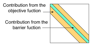
Figure 7: Configuration of the approximate Hessian for PR channels.

VI-C Solving the Newton equation

The most time consuming part of the Newton method is the determination of the Newton step, which is required to solve the Newton equation $G\mbox{\boldmath$d$}=-\mbox{\boldmath$g$}$. We here discuss how to solve the Newton equation efficiently in an inner-loop process.

VI-C1 Cholesky decomposition

If the approximate Hessian is a positive definite symmetric matrix, Cholesky decomposition is applicable to solve the Newton equation. For a given $n\times n$ positive definite matrix $M$, Cholosky decomposition decomposes $M$ as $M=LL^{t}$ where $L$ is a lower triangular matrix. A linear equation $M\mbox{\boldmath$x$}=\mbox{\boldmath$b$}$ can be solved in an efficient way by using a combination of Cholesky decomposition and backward/forward substitutions [8].

In the case of PR channels, the approximate Hessian becomes a symmetric positive definite matrix, and so we can employ Cholesky decomposition to solve the Newton equation. Fortunately, Cholesky decomposition can be accomplished with time complexity $O(n)$ for a matrix having the form shown in Fig.7. Since the backward/forward substitutions require only $O(n)$-time, the Newton equation can be solved with time complexity $O(n)$. This approach may be suitable for software implementation of the interior point decoding since Cholesky decomposition is a serial-type algorithm.

VI-C2 Jacobi method

The Jacobi method is an iterative method for solving a linear equation $M\mbox{\boldmath$x$}=\mbox{\boldmath$b$}$ [8]. This method is especially suitable for the case where the coefficient matrix $M$ is sparse. The details of the Jacobi method are as follows. The linear equation $M\mbox{\boldmath$x$}=\mbox{\boldmath$b$}$ can be rewritten in the following form:

$$(L+U+D)\mbox{\boldmath$x$}=\mbox{\boldmath$b$},$$ (82)

where $L$, $U$ and $D$ are lower triangular, upper triangular and diagonal matrices, respectively. Equation (82) can be transformed to

$$\mbox{\boldmath$x$}=D^{-1}(\mbox{\boldmath$b$}-(L+U)\mbox{\boldmath$x$}).$$ (83)

We can regard equation (83) as an update rule of $x$ and thus obtain the following recursive formula:

$$\mbox{\boldmath$x$}^{(k)}=D^{-1}(\mbox{\boldmath$b$}-(L+U)\mbox{\boldmath$x$}^{(k-1)}).$$ (84)

Starting from an appropriate initial value $\mbox{\boldmath$x$}^{(0)}$, we can evaluate the above recursive formula iteratively. If certain conditions are met, $\mbox{\boldmath$x$}^{(k)}$ eventually converges to the solution of the linear equation $M\mbox{\boldmath$x$}=\mbox{\boldmath$b$}$.

Sometimes the Jacobi method fails to converge when the matrix $M$ is not diagonally dominant. Under relaxation (UR) of the Jacobi method yields convergent results for a wider class of linear equations, including those that cannot be treated with by the original Jacobi method. The update rule for the UR Jacobi method is given by

$$\mbox{\boldmath$x$}^{(k)} = \omega\mbox{\boldmath$y$}^{(k)}+(1-\omega)\mbox{\boldmath$x$}^{(k-1)}$$ (85)

$$\mbox{\boldmath$y$}^{(k)} = D^{-1}(\mbox{\boldmath$b$}-(L+U)\mbox{\boldmath$x$}^{(k-1)}).$$ (86)

where $\omega$ is a real constant in the range $0<\omega<1$.

The Jacobi method with under relaxation is appropriate for application to solving the Newton equation. This method requires $O(n)$-time if the coefficient matrix is sparse (the number of non-zero elements in the matrix is $O(n)$) and the number of iterations is fixed. The Jacobi method is an algorithm of parallel type, and so should be suitable for a hardware implementation that can utilize its massive parallelism.

VI-D Decoder architecture

Figure 8 shows a possible hardware architecture of the interior point decoder using the Newton method. There are five major processing blocks given by approximate gradient computation, approximate Hessian computation, Jacobi solver, feasibility check, and built-in min-sum decoder. Every block is suitable for parallel implementation. In order to design a high-speed decoder, this parallelism must be exploited.

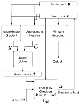
Figure 8: A possible decoder architecture of the proposed interior point decoder.

VII Behavior of interior point decoding

In this section, the behavior of the interior point decoding is discussed on the basis of the results of computer simulations. In the following simulations, a regular LDPC code with parameters $n=204,m=102,w_{c}=3,w_{r}=6$ is assumed where $w_{c}$ and $w_{r}$ denote column and row weight, respectively. The code is due to MacKay [7]. The channels used in the simulation are PR channels.

VII-A Objective function values as a function of number of iterations

Figure 9 presents the average values of the objective function $f(\mbox{\boldmath$x$})$ as a function of the number of iterations. The two curves in Fig.9 correspond to the results of the proposed scheme obtained using the gradient descent-inner loop and the Newton-inner loop, respectively. The number of iterations is defined as the number of executions of the inner loop in the decoding process. These curves have been obtained by taking the average of 1000 trials (1000 codewords).

$I_{max}=5,O_{max}=10,t_{0}=5.0,\alpha=2.0$, $h_{0}=1.0,h_{1}=-1.0,SNR=8$ dB, average of 1000 trials

Figure 9: Values of the objective function: gradient descent and Newton methods.

The parameters of the decoder are as follows: $I_{max}=5,O_{max}=10,t_{0}=5.0,\alpha=2.0$. The channel is the dicode channel (i.e., $h_{0}=1.0,h_{1}=-1.0$) with an SNR of $8$dB. It may be observed that the average objective function values decreases rapidly in the first few iterations. The curve of the gradient descent method shows the fastest decrement when the number of iterations is small (such as 1–3) . However, the Newton method (with Cholesky decomposition) gives smaller objective function values following the 4th iteration. These results suggest that the proposed decoding algorithm using the Newton method may require fewer iterations compared with that employing the gradient descent method.

We next consider the balance of the number of inner/outer loops. In the following experiment, the product of the number of inner and outer loops is set to be 50. Three combinations $(I_{max},O_{max})=(1,50),(5,10),(10,5)$ have been tested, where the interior point decoding using the Newton method with Cholesky decomposition has been used. Figure 10 presents the objective function curves for the three combinations, where the parameters of the decoder are included in the figure. We can see that the pair $(I_{max},O_{max})=(5,10)$ gives the smallest values after the 7th iteration.

$t_{0}=5.0,\alpha=2.0$,

$h_{0}=1.0,h_{1}=-1.0,SNR=8$ dB, average of 1000 trials

Figure 10: Balance of the number of inner and outer loops.

Figure 11 plots the dependency on the scale parameter $\alpha$. Again, the interior point decoding using the Newton method with Cholesky decomposition is adopted. It is observed that the convergence properties of this method are not so sensitive to the choice of the scale factor $\alpha$.

$I_{max}=5,O_{max}=10,t_{0}=5.0$,

$h_{0}=1.0,h_{1}=-1.0,SNR=8$ dB, average of 1000 trials

Figure 11: Dependency of convergence on scale factor $\alpha$.

VII-B Bit error probability of the interior point decoding

In this subsection, the bit error probability curves of the interior point decoding obtained from computer simulations are presented. The code used in the simulations is a regular LDPC code with parameters $n=204,m=102,w_{c}=3,w_{r}=6$.

In order to make a comparison with conventional decoding algorithms, we also obtained results using the joint message passing decoding (abbreviated as joint MPD) in this paper. The block diagram of the joint MPD is presented in Fig.12. The joint MPD consists of two parts: BCJR (Bahl, Cocke, Jelinek and Raviv) algorithm [9] for a PR channel and min-sum algorithm (with dump factor 0.7) for an LDPC code. The BCJR algorithm computes extrinsic information in the standard way and passes this information to the min-sum algorithm. The min-sum algorithm uses the output from the BCJR algorithm as a priori information. The extrinsic information generated from the min-sum algorithm is then treated as a priori information in the BCJR algorithm. The two parts of this method are iteratively executed in turn. We assume that the maximum number of iterations in the min-sum decoder is 10 and that the overall iterations are limited to 20. For each iteration, a parity check procedure is executed; the iteration stops when the parity check passes.

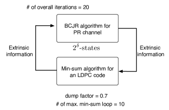
Figure 12: Block diagram of joint message passing decoding (joint MPD).

Figure 13 shows the BER (Bit Error Rate) curves for the $1-D$ channel ($h_{0}=h_{1}=1$). In this figure, the decoding performances of the interior point decoding using the gradient descent and the Newton methods are compared. For example, the label ”gradient (5,5)” corresponds to the gradient descent method with $(I_{max},O_{max})=(5,5)$. The parameters $t_{0}=5.0$ and $\alpha=2.0$ are used in these simulations. The maximum number of iterations in the built-in min-sum decoder is $L_{max}=20$ and the dump factor is $\kappa=0.7$. Comparing the gradient descent $(5,5)$ and the Newton $(5,5)$ results, Newton (5,5) exhibits much smaller bit error probabilities (approximately 2dB gain at BER = $10^{-3}$) than those of gradient (5,5). This difference could be a consequence of the faster convergence of the Newton method.

From Fig.13, it can be observed that a large improvement in BER can be obtained by increasing $I_{max}$ from 5 to 20 in the case of the gradient descent method. On the other hand, only negligible improvement is achieved by increasing $I_{max}$ from 5 to 20 in the case of the Newton method. From these observations and other simulation results, we may be able to conclude that the interior point decoding using the Newton method requires at least 5 inner-iterations to achieve most of the potential performance. By contrast, the interior point decoding using the gradient descent method requires at least 20 iterations (however, more than 20 iterations offers only a marginal improvement).

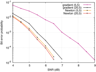
Figure 13: BER curves of interior point decoding for $1-D$ channel (1).

Figure 14 presents BER curves of gradient (20,5), Newton (5,5), and joint MPD. The channel is also a $1-D$ channel, as in the case of Fig.13. From Fig.14, firstly, we can see that interior point decoding yields a better decoding performance than that of joint MPD. The difference is approximately 1.5dB (Newton v.s. joint MPD) at bit error probability $10^{-4}$. Secondly, it is observed that Newton method gives smaller bit error probabilities than those obtained by using the gradient descent method.

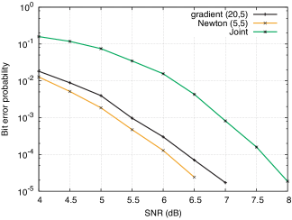
Figure 14: BER curves of interior point decoding for $1-D$ channel (2).

Figure 15 shows BER curves for a long tail PR channel $(\delta=16)$. Note that joint MPD cannot be applied to such a PR channel with large number of states (i.e., PR channel with long tail PR coefficients) because of the huge computational costs of BCJR computation, and so Fig.15 does not include the BER curve for joint MPD. The PR coefficients of this long tail PR channel are

$$\{h_{0},h_{2},\ldots,h_{16}\}=$$

$$\begin{array}[]{rrrrrr}\{1.000,&0.253,&-0.293,&0.084,&-0.057,&0.992,\\ -1.438,&-0.910,&0.106,&-0.600,&-0.844,&0.018,\\ 0.197,&-0.743,&0.490,&-0.070,&1.43\}.&\\ \end{array}$$ (90)

The coefficients $\{h_{1},\ldots h_{16}\}$ are samples of a Gaussian random variable with mean 0 and variance 1. We can see that the interior point decoding certainly has the capability to decode a given received vector observed from such a long tail PR channel. This can be considered as an advantage of the interior point decoding. Comparing the results of the gradient (20,5) and Newton (5,5) methods, the latter gains approximately 1.5 dB gain at a bit error probability of $10^{-5}$.

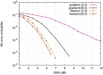
Figure 15: BER curves of interior point decoding for a long tail PR channel $(\delta=16)$.

Figure 16 deals with the case of an EPR4 channel $(\delta=3,h_{0}=h_{1}=1,h_{2}=h_{3}=-1)$. In this case, among three decoding algorithms (gradient descent (20,5), Newton (5,5), and joint MPD), joint MPD yields the best decoding performance. A large gap (1.8dB at BER $=10^{-4}$) exists between the BER curves of joint MPD and Newton (5,5). This performance degradation may be explained from the geometrical view point. Some vertices of the mapped polytope associated with this channel would have a very thin decision region.

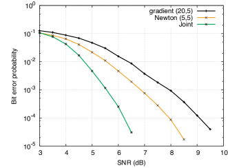
Figure 16: BER curves of interior point decoding for an EPR4 channel $(h_{0}=h_{1}=1,h_{2}=h_{3}=-1)$.

Figure 17 presents the case where the PR coefficients are $(h_{0}=h_{1}=h_{2}=1,h_{3}=-1)$. This channel and the EPR4 channel have the same degree, $\delta=3$, with the channels differing only in the sign of the coefficient $h_{2}$. From Fig.17, we can see that interior point decoding offers smaller bit error probabilities than those of joint MPD across the entire range of SNR. These results suggest that the decoding performance of the interior point decoding is highly dependent on the PR coefficients of the channel.

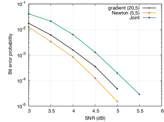
Figure 17: BER curves of interior point decoding for another $\delta=3$ channel $(\delta=3,h_{0}=h_{1}=h_{2}=1,h_{3}=-1)$.

Table I presents the throughput of the software implemented decoders. Here the throughput of the decoder is defined as the number of codewords tested in a second. Namely, it includes the time for encoding, noise generation, and decoding. It is fair to say that the values of throughput highly depend on the implementation and thus it should be considered as rough estimates of the decoding complexity. From Table I, we can observe that the proposed algorithm gives a higher throughput than that of joint MPD. It is also interesting to see that Newton (5,5) achieves a much higher throughput than that of gradient descent (20,5). This improvement on throughput is mainly due to the faster convergence of the Newton method, which can compensate the additional complexity (solving the Newton equation) required by this method. Note that a throughput of 1715 blocks/sec corresponds to 583 $\mu$ second per codeword.

TABLE I: Throughput of Software Implemented Decoders.

decoder	throughput (blocks/sec)
gradient descent (20,5)	706
Newton with Cholesky (5,5)	1715
Newton with Jacobi (5,5)	1506
joint MPD	359

Channel: $1-D$ channel, SNR = 6 dB

Code: $n=204,m=102,w_{c}=3,w_{r}=6$

Computer environment: Mac Pro with intel Xeon 2.0 GHz

VIII Conclusion

In this paper, the interior point decoding for linear vector channels is presented. The proposed algorithm is based on the principle of a relaxed MLD rule which is a convex optimization problem. Approximate variations of the gradient descent and the Newton methods play a key role in the interior point algorithm to solve the convex optimization problem. Several efficient implementation techniques have been developed in order to realize a decoder with reasonable computational complexity. The proposed algorithm may be applicable to various kinds of channels with memory, such as channels with additive correlated noise, MIMO channels, and 2D-ISI channels.

Error analysis based on the geometrical properties of the fundamental polytope is given as well. The decision regions of a relaxed ML decoder can be characterized by the normal cones of the affine image of the fundamental polytope. This geometrical view helps us to understand the behavior of a sub-optimal relaxed ML decoder based on convex optimization.

As a matter of fact, we cannot simply conclude that the optimization approach is superior to the message passing approach. There are some cases where joint MPD overcomes the proposed algorithm (e.g, EPR4 case). Furthermore, there exist other configurations of a joint MPD (see [12]) which have not been tested in this paper.

However, the simulation results presented in the previous section are encouraging and they show the potential of the optimization approach. Compared with a conventional joint MPD, the proposed decoding algorithm achieves better BER performance with less decoding complexity in the case of PR channels in many cases. An advantage of the proposed algorithm is that it is capable of handling the channels with long memory.

The present paper discusses a scheme based on a relatively simple interior point algorithm (i.e., barrier function method). More sophisticated convex optimization algorithms with faster convergence property [4] [15] can be considered in future. For example, recently, Vontobel [6] presented a new interior point algorithm for linear programming decoding. The algorithm is based on the primal-dual interior point algorithm which appears promising in terms of the convergence speed.

The efficient implementation techniques (fast feasibility check, approximate gradient, approximate Hessian) developed in this paper and the formulation of the barrier function representing the fundamental polytope could be useful not only in the proposed algorithm but also in forthcoming decoding algorithms based on various types of the interior point algorithm.

References

- [1] R.G.Gallager, ”Low density parity check codes, ” MIT Press 1963.
- [2] C.H. Papadimitriou and K. Steiglitz, ”Combinatorial optimization: algorithm and complexity,” Dover, 1998.
- [3] J. Feldman, gDecoding error-correcting codes via linear programming, h Massachusetts Institute of Technology, Ph. D. thesis, 2003.
- [4] S.Boyd and L. Vandenberghe, ”Convex optimization,” Cambridge University Press, 2004.
- [5] M.H.Taghavi and P.H.Siegel, ”Equalization on graphs: linear programming and message passing,” Proceedings of International Symposium on Information Theory, Nice, 2007.
- [6] P.O.Vontobel, ”Interior-point algorithms for linear-programming decoding,” arXiv:0802.1369v1, Feb.2008.
-
[7]
D.J.C. MacKay,
“Encyclopedia of sparse graph codes,”
http://www.inference.phy.cam.ac.uk/mackay/codes/data.html - [8] W.H. Press, B.P. Flannery, S.A. Teukolsky, W.T. Vetterling, ”Numerical recipes in C: the art of scientific computing,” Cambridge University Press, 1992.
- [9] L.Bahl, J.Cocke, F.Jelinek, and J.Raviv, ”Optimal decoding of linear codes for minimizing symbol error rate”, IEEE Transactions on Information Theory, vol. IT-20, pp.284-287, March, 1974.
- [10] A.P. Worthen, W.E. Stark: Unified design of iterative receivers using factor graphs, IEEE Transactions on Information Theory vol.IT-47, pp.843-849, 2001.
- [11] J.Garcia-Frias and J.Villasenor, ”Turbo decoding of Gilbert-Elliot channels,” IEEE Trans. on Communications, vol.COM-50, no.3, pp.357–363, 2002.
- [12] B. Kurkoski, P. Siegel, J. Wolf; ”Joint message-passing decoding of LDPC codes and partial-response channels,” IEEE Transactions on Information Theory, vol. IT-48, pp 1410-1422, June 2002,
- [13] J.Chen, M.P.C.Fossorier, ”Density evolution for two improved BP-Based decoding algorithms of LDPC codes,” IEEE Communications Letters, Volume 6, pp.208 - 210, Issue 5, May 2002.
- [14] M.Fukushima, ”Hisenkei saitekika no kiso (in Japanese, Basics on non-linear optimization),” Aasakura-shoten, 2004.
- [15] D.P.Bertsekas, ”Nonlinear programming, ” 2nd edition,, Athena Scientific, 1999.