Augmented Sparse Reconstruction of Protein Signaling Networks.

Abstract

The problem of reconstructing and identifying intracellular protein signaling and biochemical networks is of critical importance in biology today. We sought to develop a mathematical approach to this problem using, as a test case, one of the most well-studied and clinically important signaling networks in biology today, the epidermal growth factor receptor (EGFR) driven signaling cascade. More specifically, we suggest a method, augmented sparse reconstruction, for the identification of links among nodes of ordinary differential equation (ODE) networks from a small set of trajectories with different initial conditions. Our method builds a system of representation by using a collection of integrals of all given trajectories and by attenuating block of terms in the representation itself. The system of representation is then augmented with random vectors, and $l_{1}$ minimization is used to find sparse representations for the dynamical interactions of each node. Augmentation by random vectors is crucial, since sparsity alone is not able to handle the large error-in-variables in the representation. Augmented sparse reconstruction allows to consider potentially very large spaces of models and it is able to detect with high accuracy the few relevant links among nodes, even when moderate noise is added to the measured trajectories. After showing the performance of our method on a model of the EGFR protein network, we sketch briefly the potential future therapeutic applications of this approach.

Keywords: sparse representations, protein interaction models, biochemical pathways.

1 Introduction

The problem of reconstructing a network of interacting variables from a small set of data generated by the network itself has attracted considerable attention especially since this problem arises so naturally in genomics, proteomics and more generally system biology problems (see for example [Voit 2000], [Chou et al. 2006], [Husmeier 2003], [Rogers et al. 2005], [Nachman et al. 2004], [Gardner et al. 2003]). In particular, the ability to reconstruct and identify intracellular protein signaling and biochemical networks is of critical importance in modern biology. However, the ability to dynamically measure and collect enough data from every protein/node within the network is impossible with current methodologies. We sought to develop a mathematical approach to this problem using one of the most well-studied and clinically important signaling networks in biology today, the epidermal growth factor receptor (EGFR) driven signaling cascade [Araujo et al. 2005].

Interestingly, it is widely believed, and proven in some cases, that biological networks are scale free networks with a few variables (hubs) very connected to many others and most variables interacting only with a few others [Albert 2005]. Even the hubs do not interact with more than a dozen other variables in most reliable models, so that effectively we can say that these networks are sparse, with respect to the total number of all possible connections among variables. Such information can greatly help in reconstructing the network itself, as shown in [Gardner et al. 2003], [Yeung et al. 2002], [Tegner et al. 2003].

Many current algorithms to reconstruct networks from expression data are based on the application of powerful Bayesian methods after the seminal work in [Friedman et al. 2000], but, as noted in [Rogers et al. 2005] (see also [Zak et al. 2002]), these methods do not perform well with the limited amount of data that can be generated by microarray technologies. This limitation is especially pertinent for protein expression data. The other widely used approach for network reconstruction is based on parameter estimation of dynamical system models of the networks themselves [Voit 2000]. The fundamental difficulty of such approach is the very large number of parameters and reaction rates that need to be estimated [Chou et al. 2006], and this, again, leads to an inability to work efficiently with the limited data generated by microarrays and time series of expression profiles. Another viable alterative when analyzing microarray data is to simply perform some type of clustering analysis such as hierarchical or $K$-means clustering [Kaufman et al. 2005], or the recent exemplars clustering technique [Frey et al. 2007]. Clustering techniques do not require very large data sets to be applied, but they only identify similarly activated variables, and do not provide a causal understanding of the network structure.

To address the need for specialized network reconstruction methods that can work for the limited data generated by experiments, we restrict our attention in this work to ordinary differential equation (ODE) models of protein signaling networks of the form $\dot{x}=f(x)$, where $x$ is the vector of variables in the system and $\dot{x}$ its componentwise derivative. While assuming the plausibility for biological networks of a dynamical system model is a well established approach in the literature ([Voit 2000],[Chou et al. 2006]), we believe that exact modeling and parameter estimation for such models is not the most efficient way to find how quantities interact in biological systems, partly because parameter estimation is so difficult in noisy environments and with small data sets to work with. In addition, biological systems adapt their very network structure over time, especially in the presence of diseases. It is likely more effective to search for equivalent, indistinguishable, classes of models [Judd et al. 2004] that project to the same network structure, in the sense that they give rise to trajectories that are qualitatively similar and they have similar overall topology of the connections among nodes

With this general approach in mind, we ask in this paper the following question: whether the structure of sparse ODE networks can be inferred from a small set of trajectories with different initial conditions generated by the system itself. We show that, for a specific realistic case of ODE modeling of protein networks, it is possible to expand and adapt ideas from the theory of sparse regression (lasso) and signal reconstruction by $l_{1}$ minimization ([Tibshirani 1996], [Chen et al. 1998], [Hastie et al. 2001] chapter 3, [Donoho 2006a]), to develop a method that reconstructs a significant portion of these networks with good accuracy even in the presence of moderate noise of intensity up to $20\%$ of the maximum values of the trajectories. Our method builds a system of representation by using a collection of integrals of all given trajectories and by attenuating block of terms in the representation itself. The system of representation is then augmented with random vectors, and $l_{1}$ minimization is used to find sparse representations for the dynamical interactions of each node. Augmentation by random vectors is crucial in the context of network reconstruction, since sparsity alone is not able to handle the large error-in-variables in the representation when trajectories are very noisy.

One of the main strengths of our method is the ability to sharply distinguish relevant links, so that the rate of false links that are detected can be made very low. This is important in practice since it is difficult and expensive to follow up and validate experimentally potential links among proteins that are inferred by computational means [Hu et al. 2006].

The paper [Yeung et al. 2002] is a significant antecedent to our work, since in that paper the authors use a hybrid singular value decomposition (SVD) and $l_{1}$ minimization to find a sparse linear model that fits oligonucleotide microarray data. The $l_{1}$ minimization is used in that paper as a postprocessing of the reverse-engineering performed by the SVD. A similar preconditioning for large models is implemented in the recent paper [Debashis et al. in press] and applied to several examples including microarray data. In this paper we will show how $l_{1}$ minimization methods can be modified to directly approach network reconstruction and model identification problems, without any preprocessing, for realistic, very limited sampling of the data and significant noise levels, even when large spaces of non-linear models are considered. Moreover the results for the EGFR network show that our method can recover the topology of relatively small protein networks. We do not require explicit estimation of the noise level in the trajectories and we do not need multiple trajectories with same initial conditions to estimate the true trajectories in the presence of noise.

In section 2 we show how to apply $l_{1}$ minimization methods to reconstruct sparse ODE networks, stressing the specific steps that are necessary in the network setting. In section 3 we apply the algorithm sketched in section 2 to one particular protein network, the EGFR model as described in [Araujo et al. 2005].

We do not explore the biological significance of this network, strongly related to cell proliferation, but we mention here that it plays a significant role in cancer development [Lacouture 2006], so it is considered an ideal target for fine tuned potential therapies that do not impact the body at the systemic level. We will briefly mention some possible directions of research related to the medical applications of network mapping at the end of the paper.

2 Methods

2.1 Sparse Signal Processing

Suppose we have a discrete function $F(n)$, $n=1,...,N$ and a collection of functions $\mathcal{G}=\{g_{1}(n),...,g_{M}(n),\,\,n=1,...,N\}$ with $M>>N$. Then in general the representation of $F$ in terms of $\mathcal{G}$ will not be unique, meaning that there will be many ways to write $F$ as $F(n)=\sum_{m=1}^{M}a_{m}g_{m}(n)$, $n=1,...,N.$ An important question when trying to extract the significant features of $F$ with respect to $\mathcal{G}$ is to find, among the many possible representation of form as in equation (1), the one that is the most ‘sparse’, that is the representation that has as many zero coefficients $a_{m}$ as possible. This problem is in general very difficult, but we can use linear programming techniques to find approximate sparse representations, that is, representations that have just a few large coefficients and many very small ones.

We briefly introduce this type of approximation to sparse solutions here following mostly [Mallat 1998], section 9.5.1 and we refer to [Tibshirani 1996], [Chen et al. 1998], [Hastie et al. 2001], [Donoho 2006a] and [Donoho 2006b] for a thorough analysis of the relations between $l_{1}$ optimization and sparsity. The key idea is to realize that if we minimize the 1-norm of the coefficients $|a|=\sum_{m=1}^{M}|a_{m}|$, this implies that the total energy of the coefficients is concentrated in just a few of them. We can gain an intuition on this by noting that a minimization of the 1-norm reduces cancellations among different elements of $\mathcal{G}$, since these cancellations increase the 1-norm.

Note that the problem $\min(\sum_{m=1}^{M}|a_{m}|),$ subject to $F(n)=\sum_{m=1}^{M}a_{m}g_{m}(n)$, $n=1,...,N$, is equivalent to the problem $\min(\sum_{p=1}^{2M}x_{p})$, subject to $F(n)=\sum_{p=1}^{M}x_{m}g_{m}(n)-\sum_{p=M+1}^{2M}x_{m}g_{m}(n)$, with $x_{p}>0$ for every $p=1,...,2M$ and $x_{p}-x_{p+M}=a_{p}$. The linear optimization problem defined by the last two equations can be easily put in the standard format of linear programming problems, so that a solution can be quickly obtained using one of several algorithms [Lustig et al. 1994].

Given therefore a discrete signal of length $N$ and a collection of $M$ signals $\mathcal{G}$ with $M>>N$ we can easily find approximate sparse representations for $F$ in $\mathcal{G}$. This result, first exposed in [Chen et al. 1998], was the inspiration of a series of works that showed the great potential of $l_{1}$ minimization in signal processing, see for example the recent work in [Candes et al. 2004], [Candes et al. 2006]. Regression using $l_{1}$ optimization has also been used extensively and to great effect in statistical learning for model identification under the name of lasso, after the pioneering work in [Tibshirani 1996], see [Hastie et al. 2001] chapter 3 for a up to date review of use of the technique.

We will see in the next subsection the crucial adjustments that are required to make $l_{1}$ optimization effective and robust in network reconstruction problems.

2.2 Augmented Sparse Networks

Let us now write explicitly the general form of the dynamical systems of interest. Signaling networks arising from protein interactions, even though often nonlinear, are often modeled with differential equations that contain simple analytical forms that contain power function terms of variables $x_{1},...,x_{N}$ of the type $x^{\alpha}=x_{1}^{\alpha_{1}}x_{2}^{\alpha_{2}}...x_{n}^{\alpha_{n}}$, and hyperbolic terms of the type $\frac{x_{i}}{C+x_{i}}$, that take into consideration the presence of slow enzymatic kinetics (see [Voit 2000], [Araujo et al. 2005] and references therein). The assumption of sparsity of links among the nodes implies that many of the $\alpha_{i}$ are actually zero. In this paper we assume for simplicity that the right hand side of the dynamical system that we try to model has polynomial terms up to degree $d=2$, and hyperbolic terms $\frac{x_{i}}{C+x_{i}}$, $C>0$, more specifically we sample $C$ at uniform intervals of length $\bar{c}$ in a range $[0,S\bar{c}]$ of interest with $S$ some large positive integer. If we denote by $\dot{x}_{i}$ the time derivative of $x_{i}$, we consider models of the form:

$$\dot{x}_{n}=a_{0}+\sum_{i=1}^{N}a_{i}x_{i}+\sum_{i=1}^{N}\sum_{j=1}^{N}b_{ij}x_{i}x_{j}+\sum_{i=1}^{N}\sum_{s=1}^{S}\frac{x_{i}}{s\bar{c}+x_{i}}$$ (1)

where $n=1,...,N$. We can in principle consider a model that contains on the right had side all monomials $x_{i}^{\alpha_{i}}$, all binomials $x_{i}^{\alpha_{i}}x_{j}^{\alpha_{j}}$, all the way to $x_{1}^{\alpha_{1}}x_{2}^{\alpha_{2}}...x_{n}^{\alpha_{n}}$, where the exponents have norm $|\alpha_{i}|$ less than a constant $A$ and we assume a uniform sampling of the exponents. This would be a general setting compatible with the modeling approach taken in [Voit 2000], however, the main complication of such general models is already severe in our quadratic model with hyperbolic terms: when we have many nodes in the network, the combinatorial explosion of terms makes parameter fitting very difficult in the case only a limited amount of data is available on the dynamics of each node.

A possible way to approach the fitting problem implicit in equation (1) is to find the model that minimize the $l_{1}$ norm of the parameters of the terms in the equation. From the background material summarized in the previous subsection, we know that $l_{1}$ optimization leads to a sparse representation of signals with very few terms with non-zero parameters, and that the optimization itself can be performed with linear programming techniques [Chen et al. 1998] .

Since we noted in the introduction that actual biological networks are generally sparse, the $l_{1}$ fitting method should, in principle, improve our ability to find the actual links among nodes. Exact parameter fitting is difficult in this case as well and we will see in the results section that direct application of the $l_{1}$ fitting as used in signal processing leads to very poor results.

To be specific, we assume that we sample variables $x_{1},...x_{N}$ and that we have several trajectories $x_{n,r}$ $r=1,...,R$ with $R$ different initial conditions. We denote by $\dot{x}_{1},...,\dot{x}_{N}$ the respective derivatives at each of the sampled points. If we write $X_{n}=[x_{n,1},...,x_{n,R}]$, $\dot{X}_{n}=[\dot{x}_{n,1},...,\dot{x}_{n,R}]$, and we denote by $J$ the unit vector of same length as $X_{i}$, a formal substitution in equation (1) of $x_{n}$ with $X_{n}$ and $\dot{x}_{n}$ with $\dot{X}_{n}$ leads in effect to a problem of representation of discrete signals $\dot{X}_{n}$ in terms of the collection of signals $\mathcal{X}=\{J,X_{i},X_{j}X_{k},\frac{X_{i}}{s\bar{c}+X_{i}}\}$ with $i,j,k=1,...,N$, $s=1,...,S$. This way of stating the problem of reconstructing a specific network of the form (1) highlights the potential of applying the $l_{1}$ sparsity techniques to recover the effective system from a collection of different trajectories. Now the first requirement for applying the $l_{1}$ method is to have an underdetermined system with the cardinality $M$ of $\mathcal{X}$ such that $M>>L$, where we denote by $L$ the length of vectors in $\mathcal{X}$. However a direct application of $l_{1}$ optimization to the network data will not work in the presence of high noise and for very limited data. As much as sparsity is a powerful device to explore signal representations, it is not able by itself to deal with the large error-in-variables in the representation generated by the system trajectories. There are some crucial modifications that are necessary to get useful reconstruction results on protein networks, we term them model augmentation, attenuation of blocks of terms, and integral modeling.

Model Augmentation with Random Terms: The main issue that prevents an accurate reconstruction of the network is the presence of noise in the trajectories. Because of such noise the representation system needs to account for large errors-in-variables [Voss et al. 2004] when fitting the models on the noisy data. To gain a better sense of this problem, denote the noisy measurements of $X_{i}$ and $X_{j}$ as $\tilde{X}_{i}=X_{i}+N_{i}$ and $\tilde{X}_{j}=X_{j}+N_{j}$ respectively, and assume that the differential model includes a term $X_{i}X_{j}$ in the representation of some $\dot{X}_{n}$. This means that when we represent $\dot{X}_{n}$ in $\mathcal{X}$ we do not just want a sparse representation, but we would like the term $\tilde{X}_{i}\tilde{X}_{j}$ to appear in that specific representation with large non zero coefficient. Now $\tilde{X}_{i}\tilde{X}_{j}=X_{i}X_{j}+X_{i}N_{j}+X_{j}N_{i}+N_{i}N_{j}$, and we would like the noisy residue $X_{i}N_{j}+X_{j}N_{i}+N_{i}N_{j}$ to ‘disappear’, i.e. to contribute marginally to the $l_{1}$ optimization. The way we approached this problem is to go from the representation in equation (1) to a representation:

$$\dot{X}_{n}=a_{0}+\sum_{i=1}^{N}a_{i}X_{i}+\sum_{i=1}^{N}\sum_{j=1}^{N}b_{ij}X_{i}X_{j}+$$ (2)

$$+\sum_{i=1}^{N}\sum_{s=1}^{S}\frac{X_{i}}{s\bar{c}+X_{i}}+\sum_{g=1}^{G}n_{g}$$

where $n_{g}$ $g=1,..,G$ are discrete random vectors normally distributed, scaled to have norm 1. We want $G$ much larger that $L$ so that the energy of noisy residues like $X_{i}N_{j}+X_{j}N_{i}+N_{i}N_{j}$ is uniformly distributed among all the random vectors $n_{g}$, and the overall contribution to the $l_{1}$ norm of these noisy residues is small. Moreover a large value of $G$ improves the conditioning of the corresponding linear programming problem and therefore the speed of convergence to the optimal solution. Note that $G$ is dependent on the particular instance of problem that is given, and more specifically on the type and number of trajectories and sample points in each trajectory, but the performance of the method we describe in this section is not strongly dependent on its specific value, as long as $G>>L$. In Figure 5 we show numerical evidence of the significance of adding random terms in the context of the epidermal growth factor receptor case study.

This extension of the basic model has far reaching consequences, since it assures that the new models are large enough to be able to perform an approximate sparse minimization, strongly retaining the dependence from the original terms of the ‘effective’, non-random model, while diffusing any potential noise in the data among the random terms of equation (2). The non-random portion of the matrix derived from the ODE network itself can be very ill conditioned. In particular, the hyperbolic terms generated by the same variable will be highly correlated among each other. There is an intrinsic inability to fully control the representation matrix generated by the trajectories and the error in variables that are bound to appear when trajectories are very noisy. This is a distinct characteristic of ODE reconstruction networks and one that makes this work diverge in methodology and outlook from standard $l_{1}$ signal reconstruction.

Attenuation of Block of terms: We seek to have reconstructed models with low complexity, that is, with terms of low degree, so it is useful to enforce a way to explicitly suppress the terms belonging to more complex blocks of terms such as quadratic and hyperbolic ones. The large number of quadratic and hyperbolic terms increases the chance, in a noisy setting, that several wrong terms from these blocks are selected in the representation of each node. By suppressing each of these blocks of terms we reduce the chance of this wrong selection and we give more weight to linear terms. Such suppression of higher complexity terms can be done by using suitable attenuation coefficients. More specifically, we choose to attenuate uniformly all terms in a block by a factor $0<\beta<1$. Assuming that all vectors of the collection of terms $\mathcal{X}$ were scaled to have $l_{2}$ norm equal to $1$, we effectively multiply their inner product with any signal by $\frac{1}{\beta}$, which is bigger than $1$, so the $l_{1}$ optimization will have the tendency to select fewer of them to chose the representation with the minimal $l_{1}$ norm. This is another interesting point specific to the modeling of networks. Empirically, we find that this adjustment is important for obtaining the very best results in the reconstruction of the geometric structure of the network, for example an attenuation of a factor of $\beta=0.5$ for both quadratic and hyperbolic terms was near optimal for the epidermal growth factor receptor network. The need of some attenuation is especially strong when we want very few selected false links and the trajectories are very noisy. We find that a wide range of small values of $\beta$ gives similar reconstruction results, but the optimal selection of $\beta$ for each different block, including a possible attenuation for the block of random terms, is an open problem and we will explore numerically this issue in a separate paper. Essentially, these attenuation coefficients are one more device to keep the errors-in-variables from generating false links in the computed representation of each node, assuming that low degree and low complexity terms are to be preferred.

Integral Modeling: In a realistic reconstruction setting we have few sample points and a relative noise that can be as high as $20\%$ in the measured trajectories, making the estimation of the derivatives very difficult. This problem transcends the specifics of our approach and is a key issue in the study of experimentally generated time series. Note that to use $l_{1}$ optimization, we clearly do not need to use only local differential information. To avoid the problem of direct estimation of derivatives in the highly noisy cases, we note that the equations as (1) can be written for $n=1,...,N$, in integral form as:

$$x_{n}(t)-x_{n}(t_{0})=a_{0}+\sum_{i=1}^{N}a_{i}\int_{t_{0}}^{t}x_{i}dt+$$ (3)

$$+\sum_{i=1}^{N}\sum_{j=1}^{N}b_{ij}\int_{t_{0}}^{t}x_{i}x_{j}dt+\sum_{i=1}^{N}\sum_{s=1}^{S}\int_{t_{0}}^{t}\frac{x_{i}}{s\bar{c}+x_{i}}dt.$$

This integral representation avoids the implicit problem of finding a good estimation of the derivative from a limited number of samples of the trajectories. The relative noise in the measurement of $x_{n}(t)-x_{n}(t_{0})$ is comparable with the relative noise of the time series $x_{n}$ itself when $t$ is far from $t_{0}$. Moreover, for biological signals derived from proteomics and genomics, variables often represent intensity or concentration profiles that always assume positive values and therefore, in these cases, we expect the integrals on the right hand side to be dominated by the integrals of the true values of the variables, when zero mean noise is added to them. A further advantage of integral modeling is that we can easily estimate multiples of the integrals on the right hand side of equation (3) by summing up the samples that are given from $t_{0}$ to $t$, if sampling is uniform. If sampling is not uniform, which is very often the case for experimental data, we can scale the contribution of each summand multiplying by the size of the corresponding sampling interval.

Note that the constant term $a_{0}$ was used simply as a term to correct potential biases in (1), as it does not carry information on the nodes’ links, so we use it similarly in (3) and we do not take its integral. The augmentation by random terms and the attenuation of blocks of terms clearly can be applied to the integral representation (3) as well. The system representation that takes into account random augmentation, attenuation of blocks of terms and integral modeling is the following:

$$x_{n}(t)-x_{n}(t_{0})=a_{0}+\sum_{i=1}^{N}a_{i}\int_{t_{0}}^{t}x_{i}dt+$$ (4)

$$+\beta_{q}\sum_{i=1}^{N}\sum_{j=1}^{N}b_{ij}\int_{t_{0}}^{t}x_{i}x_{j}dt+\beta_{h}\sum_{i=1}^{N}\sum_{s=1}^{S}\int_{t_{0}}^{t}\frac{x_{i}}{s\bar{c}+x_{i}}dt+\sum_{g=1}^{G}n_{g}.$$

where $\beta_{q}$ and $\beta_{h}$ are positive attenuation coefficients for quadratic and hyperbolic terms, both smaller than $1$. This representation is used in the actual network reconstruction algorithm that we are going to describe now.

2.3 Network Reconstruction Algorithm

The observations in the previous subsection can be gathered into a simple reconstruction algorithm based on $l_{1}$ optimization, which we call augmented sparse reconstruction. We label the variables involved in a slightly different way in the algorithm to highlight the flexibility in the choice of the input for the algorithm. Given trajectories from a sparse system that is believed to be of a certain generic form, for each discretely sampled trajectory $X_{n,r}$, $r=1,...,R$, let $\bar{X}_{n,r}$ be the vector $X_{n,r}(t)-X_{n,r}(t_{0})$ where $t$ takes all sampled values. Moreover, for a given vector $g(t)$, $t=t_{0},...,t_{L}$, let $I(g)$ be the vector whose $l$-th component is the sum $\sum_{i=0}^{l}g(t_{i})$, and let $J$ denote the unit vector. The basic process to identify the nodes is the following:

• Suppose we are given $N$ node variables and that for each variable it is possible to generate $R$ uniformly sampled trajectories $X_{n,r}$ $r=1,...,R$ with different initial conditions. Write $Y_{n}=[\bar{X}_{n,1},...,$$\bar{X}_{n,R}]$, $G_{n}=[I(X_{n,1}),...,$ $I(X_{n,R})]$, $n=1,...,N$, $G_{ij}=[I(X_{i,1}X_{j,1}),...,$$I(X_{i,R}X_{j,R})]$ and $H_{js}=[I(\frac{X_{j,1}}{s\bar{c}+X_{j,1}}),...,$ $I(\frac{X_{j,R}}{s\bar{c}+X_{j,R}})]$, $s=1,2,...,S$ and $\bar{c}$ is the sampling interval for the hyperbolic terms. For each $n=1,...,N$:

• Choose an attenuation coefficient $\beta_{q}$ for the quadratic terms and another one, $\beta_{h}$, for the hyperbolic terms. Let $n_{g}$, $g=1,..,G$, be discrete random vectors normally distributed scaled to have norm 1. Denote by $|\,|$ the $2$-norm of a vector and let $\hat{G}_{l}$ be the matrix whose columns are all the vectors $\frac{G_{i}}{|G_{i}|}$, $\hat{G}_{q}$ be the matrix whose columns are all possible vectors $\frac{G_{ij}}{|G_{ij}|}$ and $\hat{H}$ be the matrix whose columns are all allowed hyperbolic terms $\frac{H_{is}}{|H_{is}|}$. Let $N_{G}$ be the matrix whose columns are the random vectors $n_{g}$ scaled to have norm $1$. Choose $G$ large enough to have the matrix $Z=[J,\hat{G}_{l},\beta_{q}\hat{G}_{q},\beta_{h}\hat{H},N_{G}]$ with small condition number (say less that $10^{2}$).

• Find the minimal $l_{1}$ solution to the underdetermined system $Y_{n}=Z\alpha$.

• Choose a threshold $T_{n}$ and let $\alpha_{T_{n}}$ be the coefficients in $\alpha$ larger than $T_{n}$. Let $\mathcal{I}_{n}$, the estimated set of directed links of node $n$, be the union of all node indexes that appear in terms of $Z$ corresponding to coefficients in $\alpha_{T_{n}}$.

Basically in step A we use the sampled trajectories to estimate the integrals in the representation on the right hand side of equation (4). In step B we scale the terms of the representation, we attenuate quadratic and hyperbolic terms, and we augment the model with scaled random terms. In step C we apply $l_{1}$ minimization. Finally in step D we select the largest coefficients in the representation and we estimate the set of links that determine the dynamics of each node. The choice of the threshold in step D is very delicate and it is explored in depth for the epidermal growth factor receptor signaling network that we study in the next section. We stress again that by no means we need to limit ourselves to linear, quadratic and hyperbolic terms. general power function expansions or higher degree polynomial terms are possible within the frame of this method, since random terms and $l_{1}$ minimization keep the reconstruction stable even for very underdetermined systems of representation.

3 Results

3.1 The epidermal growth factor receptor (EGFR) Network

In this section we show the performance of the augmented sparse reconstruction method A-D on the epidermal growth factor receptor (EGFR) protein network described in [Araujo et al. 2005] and explicitly shown in the appendix. We again emphasize that the ability to dynamically measure and collect enough data from every protein/node within the network is impossible with current experimental methodologies. The EGFR network is one of the most well-studied and clinically important signaling networks in biology today and the ability of our method to reconstruct a model of such fundamental network is very promising. The EGFR network has been modelled in [Araujo et al. 2005] as a system involving only linear, quadratic and hyperbolic terms, so the general model in equation (1) (and therefore in equation (4)) is ideally suited for its analysis, however the right hand side of equations (1) and (4) have a very large number of quadratic and hyperbolic terms for the EGFR network, both due to the large number of variables involved, and to the need of considering a sufficiently large sampling of hyperbolic terms. Therefore already in this case we are faced with the extreme difficulty of finding the few relevant terms for the actual EGFR network. Despite this difficulty, augmented sparse reconstruction is able to find a very significant fraction of the links in the network. Moreover preliminary results show that the method is robust with respect to changes in the size and type of system of representation.

The sparsity of links for the EGFR system has some variation between nodes; we have $11$ variables with less than $4$ distinct terms (linear, quadratic or hyperbolic) in the expression for their derivative, $9$ variables with less than $8$ terms and $1$ variable, $x_{4}$, with $19$ terms. This last variable is not sparse and corresponds to the main ‘hub’ of the EGFR network.

We assume that $100$ time series with different initial condition, each of a length of $25$ points, are available for each variable in the system. Only $500$ uniformly selected points among the total $2500$ are used in the algorithm, so that we are effectively working with a very small data set of points, even though we gain some information from the missing points when estimating the integrals in equation (4). The initial conditions for each variable are chosen as uniformly distributed random numbers in the interval $[0,\,40]$. In real systems the biologically significant ranges of initial conditions vary among different variables. This raises an interesting theoretical and practical question: which is the minimal domain of initial conditions that allows the reconstruction of the network? This question is particulary relevant for networks that display simple dynamics, since each short trajectory may not carry the full information on the underlying network.

The length of the time series is chosen to be consistent with the sampling rate that can be performed in practice, that is the reason we take only $25$ uniformly spaced points in the time interval $[0,\,27]$ along each trajectory. To put this number in perspective, we note that for a time series with fast initial decay like the one in Figure 1(a) this mean that we have only $2$ to $3$ points in the high varying region of the series, while for a time series with slow decay as the one in Figure 1(b) we have a larger proportion of points where the time series has not yet relaxed to its steady state. As we already stressed, this infrequent sampling is one of the reasons we had to move from the differential representation of the network to the integral one used in A-D, as it may be problematic to estimate derivatives in such infrequent sampling scenario. The way we add noise to the trajectories is by taking the maximum $M$ of each given time series and by adding uniform white noise in the interval $[-m,\,m]$ where $m$ is equal to a fraction of $M$; this seems to give levels of noise consistent with experimental conditions. The characteristic shape of the noisy time series from the EGFR network, is shown in Figure 1 (noise level $15\%$).

The sampling interval of the hyperbolic terms is $\bar{c}=10$ and the total number of hyperbolic terms for each variable is $S=50$. The total number of terms for the model, and therefore the total number of parameters, is $1449$, far more than the $500$ data points we use to find the links for each node. The number of random vectors to be used in step B is chosen as $G=2500$. The attenuation for the quadratic and the hyperbolic terms is chosen to be $\beta_{q}=\beta_{h}=0.5$.

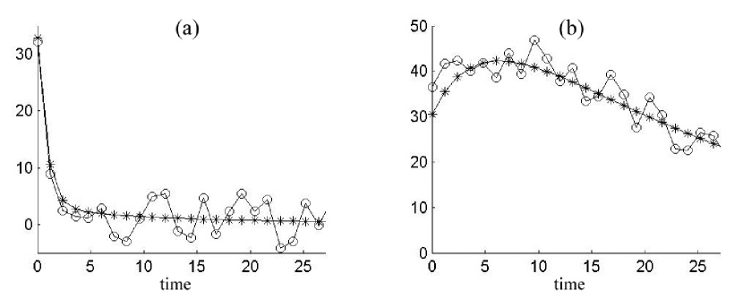
Figure 1: In subplots (a) and (b) we show typical trajectories that are observed in the EGFR system, sampled uniformly $25$ times in the time interval $[0,\,27]$. Starred curves are the actual trajectories, circled curves are the trajectories with $15\%$ relative noise added. Plot (a) shows a trajectory of $x_{9}$ that settles within few samples points to a base value, plot (b) a trajectory of $x_{6}$ with a much slower decay.

In Figure 2 we show a typical example of the sparse representation that can be obtained by applying A-D to the infrequently sampled, noisy trajectories of the EGFR network with the noise level as in Figure 1. More specifically, we show the reconstructed representation for $Y_{2}$, the vector of all integrals of $\dot{x}_{2}$ defined in step A, with respect to the integral of all linear, quadratic, and hyperbolic terms, as defined in step B. We choose variable $x_{2}$ because it has very few terms in its actual representation of the derivative, namely $\dot{x}_{2}=-0.06x_{2}+0.2x_{3}+0.003x_{1}x_{23}-0.02x_{2}^{2}$, having a sparsity for which the algorithm works often at its best. We plot the norm of the coefficients of: the linear terms in Figure 2(a), from $G_{1}$ to $G_{23}$; the quadratic terms in Figure 2(b), ordered as $G_{1,1}$,…, $G_{1,23}$, $G_{2,2}$,…, $G_{22,23}$; the hyperbolic terms in Figure 2(c), ordered as $H_{1,1}$,…, $H_{1,10}$,…, $H_{23,1}$,…, $H_{23,10}$; and the random terms in Figure 2(d).

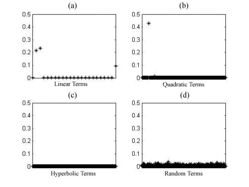
Figure 2: From top left, we plot the norm of the coefficients of $Y_{2}$ (as defined in step A) for: (a) the linear terms $\hat{G}_{l}$; (b) the quadratic terms $\hat{G}_{q}$; (c) the hyperbolic terms $\hat{H}$; and (d) the random terms.

The $3$ largest coefficients across all terms correspond exactly to three of the terms in the representation of $\dot{x}_{2}$, namely $x_{2}$, $x_{3}$ and $x_{1}x_{23}$, we are missing instead the $x_{2}^{2}$ term. The forth largest coefficient in the reconstructed representation corresponds to the $x_{23}$ term, so it repeats to some extent the information on the network linkage given by the $x_{1}x_{23}$ term. If we apply the reconstruction algorithm to this node with $20$ different realizations of $15\%$ relative noise, the $x_{2}$ term appears as dominant $18$ times, the $x_{3}$ term $15$ times, the $x_{1}x_{23}$ term $20$ times and the $x^{2}$ term $3$ times. Note that the dominance of a term is not only due to the size of its coefficient, but to the intensity of the corresponding signal as well, for example $x_{1}x_{23}$ has coefficient $0.003$ in the equation for $\dot{x}_{2}$ and yet it is recovered more often than $x^{2}$ that has larger coefficient $0.02$. We believe this has to do with the specific norm scaling that is selected in step B of the algorithm. Different choices of norm scaling may be useful to improve further the performance of the method.

The example of the reconstruction of the representation of $\dot{x}_{2}$ is typical: some terms not only may be missing, but they can be partially wrong, for example a term $x_{i}$ may appear in the representation as $x_{i}^{2}$, or a term $x_{i}x_{j}$ may be replaced by a term $x_{i}x_{k}$ that gives similar shapes for the given initial conditions. Note that these two possibilities do carry some significant information on the geometry of the network, even though the specific terms are incorrect.

We can compare at this point the effectiveness of our $l_{1}$ method in identifying the relevant links with respect to simpler techniques such as correlation. In Figure 3 we show, for comparison, the correlation $Y_{2}$ with: the linear terms in Figure 3(a), from $G_{1}$ to $G_{23}$; the quadratic terms in Figure 3(b), ordered as $G_{1,1}$,…, $G_{1,23}$, $G_{2,2}$,…, $G_{22,23}$; the hyperbolic terms in Figure 3(c), ordered as $H_{1,1}$,…, $H_{1,10}$,…, $H_{23,1}$,…, $H_{23,10}$. The most negatively correlated linear term corresponds to $x_{2}$, the most negatively correlated quadratic term to $x_{2}^{2}$, and the cluster of most negatively correlated hyperbolic terms correspond to $x_{2}$ as well. Note however that many terms show similar level of large negative correlation, especially among the quadratic terms, so that it is difficult to set a threshold on the norm of the correlation coefficients that would, for example, identify only $x_{1}x_{23}$ as another relevant term. The key point is that the considerable sparsity of the reconstructions computed by our method allows for an accurate distinction of false links and true links. We do not explore this issue further in this paper, but see our forthcoming paper for a comparison of the augmented sparse reconstruction with $l_{2}$ regression on a special class of ODE networks.

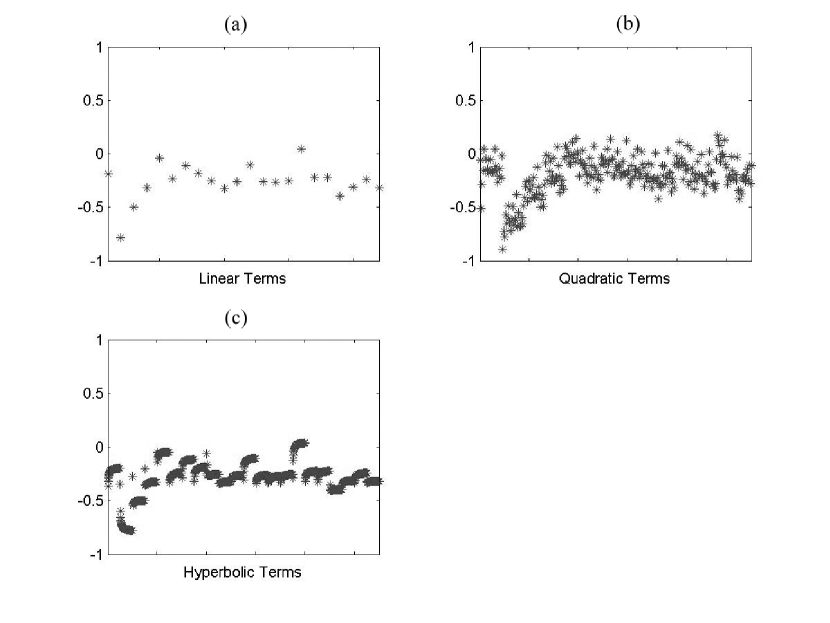
Figure 3: From top left, we plot the correlation coefficients of $Y_{2}$ (as defined in step A) with: (a) the linear terms $\hat{G}_{l}$; (b) the quadratic terms $\hat{G}_{q}$; (c) the hyperbolic terms $\hat{H}$.

To evaluate globally the quality of the reconstruction results for different levels of noise we use the ratio of computed true links with respect to the total number of true links (true positives rate) and the ratio of computed false links with respect to the total number of false links (false positives rate). An important question when assessing the quality of reconstruction is the proper estimation of the thresholds $T_{n}$ used in D. In general we expect these thresholds to vary according to the noise level in the time series, but even the sampling rate will affect our degree of confidence in the computed links so we must find an automatic way to estimate the threshold from the data. Note moreover that the threshold must be represented in terms of the coefficients used to represent each node. To this extent we define a threshold, for a given system, as a constant multiple of the standard deviation of the non-zero coefficients of the non-random terms of each node, what we may call the deterministic coefficients of the representation (in practice we neglect any coefficient with norm smaller than $10^{-10}$). Formally we define $T_{i}=K\sigma_{i}$, $i=1,...,N$, where $K$ is some fixed constant determined for the whole system, while $\sigma_{i}$ is the standard deviation of the absolute value of the deterministic non-zero coefficients of the representation of node $i$. This flexible definition of the threshold ensures that: a) the threshold level is relative to the norm of the coefficients of each node; b) the threshold is larger if there are many sizeable non-zero coefficients in the representation of a specific node. The main advantage of a uniform definition of threshold across all variables is that we need the proper estimation of a single threshold $K$, and we have the whole reconstruction data available to do that. If the network has very distinct behavior for different subsets of nodes, it may not be possible to use a single multiplier and we must resort to thresholds estimated for each node separately.

Before suggesting a specific way to find the uniform threshold $K$ from the computed representations, let us see what we would get with an ‘ideal’ choice of it. Suppose that for each noise level in the time series, we select $K$ so that the false positives rate stays below $0.1$. We perform such analysis for $20$ realizations for each level of relative noise in the trajectories from $0\%$ to $25\%$. In Figure 4(a) we can see the result of such choice of thresholds: the average true positives rate (starred curve) is high (around $0.65$) even for realistic trajectories’ noise of the order of $20\%$. For all $20$ realizations the computed true positive rates differed from the average by at most $0.054$ units, with standard deviation, at each noise level, of at most 0.026. The computed average values of $K$ are: $K_{0\%}=0.032$, $K_{5\%}=0.046$, $K_{10\%}=0.067$, $K_{15\%}=0.099$, $K_{20\%}=0.120$, $K_{25\%}=0.137$. The noisier the time series, the higher the value of $K$ needed to keep the false positives rate small.

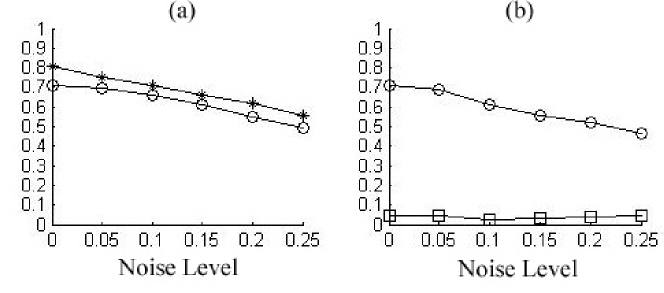
Figure 4: In plot (a) we have the average true positives rates for relative noise in the trajectories from $0\%$ to $25\%$ when the value of the threshold multiplier $K$ is artificially set to keep the false positive rate at: $0.1$ (starred curve) and $0.05$ (circled curve). In plot (b) we have the average true positive rates (starred curve) and average false positive rates (squared curve) for relative noise in the trajectories from $0\%$ to $25\%$ where the value of the threshold multiplier $K$ is found for each noise level by using the heuristic E.

Figure 4(a) shows also the average true positives rates (circled curve) when the false positives rate is kept at $0.05$. In this case, for all $20$ realizations the computed true positive rates differed from the average by at most $0.071$ units, with standard deviation, at each noise level, of at most 0.03. The computed average values of $K$ are: $K_{0\%}=0.104$, $K_{5\%}=0.129$, $K_{10\%}=0.185$, $K_{15\%}=0.253$, $K_{20\%}=0.315$, $K_{25\%}=0.369$. Even for noiseless trajectories we still do not find all true links, this is due in part to the infrequent sampling of the trajectories that hides subtle interactions among the nodes. Note that the rates we display are obtained excluding from the average the reconstruction of variable $4$ that does not have sparse representation and which is a ‘hub’, so likely to be better knwon experimentally. We decided to exclude that specific protein in our estimates of the errors because only very few proteins are believed to perform the role of hub of a network in signaling pathways, therefore we believe that the error rates computed above are a better indicator of the errors we would find in computing the representation of a generic protein in a large network. Moreover the representation of $x_{4}$ is so different from the others that the use of the same threshold multiplier for it as for all other variables does not seem appropriate. Including variable $4$ in computing the errors, without any modification in the choice of threshold multiplier, would lead true positive rates to slightly worsen.

It is possible in principle to have cases when much finer sampling of the trajectories is experimentally available. To simulate this scenario, suppose we sample the trajectories of the EGFR network uniformly $100$ times in the time interval $[0,\,27]$, then the error rates improve significantly. If we keep false positive rate to $0.1$, then average true positive rates are about $0.88$ in the absence of noise, this is a improvement of almost $0.08$ with respect to the same time series sampled uniformly only $25$ times. In Figure 5(a) we show average true positive rates for noise level from $0\%$ to $25\%$ in this fine sampling scenario. We use $20$ realizations for each noise level in computing the averages

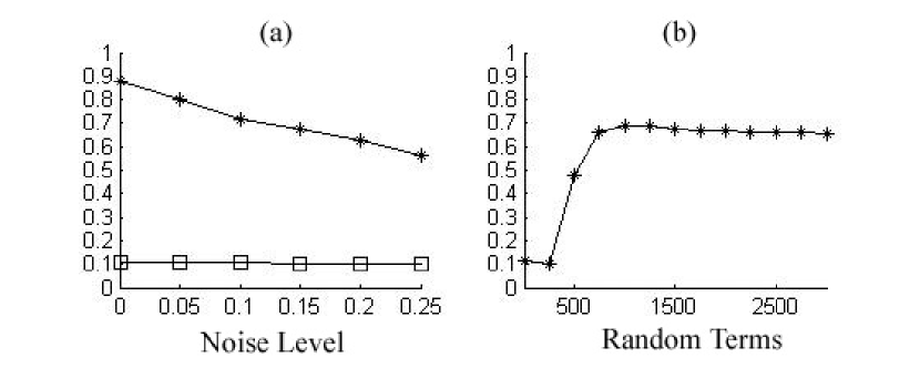
Figure 5: In plot (a) we have the true positives rates (starred curve) for relative noise in the trajectories from $0\%$ to $25\%$ when the value of the threshold multiplier $K$ is artificially set to keep the false positive rate (squared curve) at $0.1$. Network trajectories are sampled $100$ times in the interval $[0,\,27]$ to generate this plot. In plot (b) we have the true positive rates (starred curve) as a function of the number of random terms added to the model. Network trajectories used to generate this plot are sampled $25$ times in the interval $[0,\,27]$ and noise level is kept at $15\%$. The value of the threshold multiplier $K$ is artificially set to keep the false positive rate at $0.1$.

Figure 5(b) shows that a large number of random terms is important for the proper functioning of algorithm A-D. Namely we show that the average true positive rates improve when we increase the number $G$ of random terms from $0$ to $3000$ in intervals of $250$. Trajectories are sampled infrequently ($25$ times in the interval $[0,\,27]$), false positive rates are kept at $0.1$ and relative noise level is fixed at $15\%$. The true positives rate is very low, just $0.13$, when there are no random terms added. Addition of $1000$ or more terms gives high true positive rates, about $0.68$, that are comparable for several values of the number of terms $G$. These results show also the robustness of the algorithm with respect to the choice of $G$.

3.2 Choice of Threshold

We now approach the problem of finding a suitable value of $K$ from the reconstruction data generated by the algorithm itself at the end of step C. Denote by $S(K)$ the total number of selected links that are found in step D of the augmented sparse reconstruction algorithm by using thresholds $T_{n}=K\sigma_{n}$. We can split $S(K)$ as $S(K)=S_{t}(K)+S_{f}(K)$ where $S_{t}(K)$ denotes the number of true computed links and $S_{f}(K)$ the number of false computed links. Since for each node we have only a small number of true links by assumption, and their corresponding coefficients in the representation are, in general, very large, we can conjecture that, as we let $K$ increase continuously from $0$ to $\infty$, $S_{t}(K)$ will decrease very slowly at the beginning. Since $S_{t}(K)$ assumes only integer values, this slow decay will appear as infrequent small jumps, this means that the (discontinuous) derivative $dS(K)$ of $S(K)$ will be dominated by the derivative $dS_{f}(K)$ of $S_{f}(K)$ for small values of $K$ and by $dS_{t}(K)$, the derivative of $S_{t}(K)$, for larger values of $K$, therefore we can infer some of the properties of $S_{f}(K)$ which is not known, from those of $S(K)$, which is a computable function.

In Figure 6(a) to 6(c) we show approximations to $dS_{t}(K)$, $dS_{f}(K)$ and $dS(K)$ for a specific reconstruction with relative noise in the time series of the order of $10\%$. We choose a fine uniform sampling $U=0.001$ of $K$, up to $K=3.5$, so that $dS(K)$ never goes below $-2$. To have the ideal case in which $dS(K)\geq-1$ for all $K$ seems to require excessively fine sampling rate. Note that $S(K)$ is identically zero for $K>3.26$, we can also immediately see the similarity of $dS(K)$ and $dS_{f}(K)$ in the frequency of negative jumps for small values of $K$. The frequency of jumps of $dS(K)$ greatly decreases around $K=0.30$, to see this transition point more clearly, let $K_{1},...,K_{M}$ be the values of $K$, ordered from smallest to largest, for which $dS(K)\neq 0$ and define a function $J(i)=K_{i}-K_{i-1}$, $i=2,...,M$ that computes the width of negative jumps. We plot $J$ in Figure 6(d) and we can see that for $i\approx 57$ we suddenly have much wider intervals between jumps, this value of $i$ corresponds to $K_{57}\approx 0.29$. We argue that a suitable value $K_{f}$ of the multiplier $K$ is the one for which $J(i)$ has very different local averages for $i<f$ and $i>f$. To find such $K_{f}$ we can use the following rule:

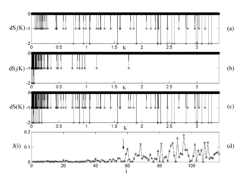
Figure 6: Plots of:(a) $dS_{t}(K)$; (b) $dS_{f}(K)$; (c) $dS(K)$ for $10\%$ relative noise in the trajectories. In plot (d) we show $J(i)$, the distance between the $i-1$-th and the $i$-th negative jumps in $dS(K)$, for $10\%$ relative noise in the trajectories. $K$ is sampled uniformly with sampling interval of size $U=0.001$. The arrow in plot (d) points to the index values, around $i=57$, for which we have a large change of mean frequency of jumps.

• Set an integer I, let $V(i)=\frac{\bar{J}_{i-I}}{\bar{J}_{i+I}}$, $i=I,...,M-I$, where we denote by $\bar{J}_{i-I}$ the mean of $J$ for values between $i-I$ and $i$ and by $\bar{J}_{i+I}$ the mean of $J$ for values between $i$ and $i+I$. Denote by $f$ the index for which $V(i)$ is minimum, and by $K_{f}$ the corresponding threshold multiplier.

Rule E uses the ratio of the local mean of the length of intervals between jumps before and after the $i$-th jump to select the jump for which the relative increase is maximum. If we use $I=20$ in E, we find from the output data of step C of the algorithm the following threshold multipliers: $K_{0\%}=0.114$, $K_{5\%}=0.164$, $K_{10\%}=0.328$, $K_{15\%}=0.415$, $K_{20\%}=0.428$, $K_{25\%}=0.486$. In Figure 4(b) we plot the average true positive rates and average false positive rates computed by using in step D of the algorithm by using these estimated values of $K$. We use $20$ realizations for each noise level in computing the averages, for all $20$ realizations the computed true positive rates differ from the averages by at most $0.11$ units, with standard deviation, at each noise level, of at most 0.058. The false positives rate is below $0.11$ for all realizations and all noise levels. With $10\%$ relative noise in the trajectories, we have a significant average true positives rate of about $0.61$ with average false positives rate of only $0.025$. There is a greater variability in true positives and false positives rates in Figure4(b) with respect to those computed in Figure4(a), this fact points out the need of a more sophisticated analysis of the change of mean frequency. For example, a wavelet maxima analysis ([Mallat 1998], chapter 6) of $J(i)$ can be used for a more robust evaluation of the thresholds. It would be of great interest to deduce theoretically the value of $K_{f}$, under suitable conditions on the class of network models.

4 Discussion

There are still many open questions whose answers will shape the way augmented sparse reconstruction methods are applied to network reconstruction. What is the limiting node sparsity that still allows the network itself to be recovered with this method? how are the error rates affected if only a subset of the variables is available? how does the network we compute on this subset of variables relates to the full network? if we have a node that is unrelated to the chosen subset of the network, it tends to have a greater portion of its norm accounted for by the random terms, and this ca be used to decide whether it is well connected to the other variables, but further research in this direction is needed.

In some cases the ‘skeleton’ of the network may be available, for example for proteins networks we may know roughly how the system is connected for healthy cells. Can we use this additional information to detect, with this method, whether patients with cancer develop additional strong links among nodes? Preliminary evidence suggests that small new links that do not make the system unstable are often detectable, but it would be interesting to use the available information on the skeleton of the network directly in the algorithm.

Even when previous information on the network is not available, it is very important for clinical applications to determine whether a specific protein has very distinct representations for cancerous cells and for healthy ones. If this is the case, then the reconstruction algorithm can predict changes in the signaling pathways that are likely due to the cancer itself.

One possible extension of our method is to perform the estimation of links only on local subsets of trajectories. This local application of the algorithm may highlight different links that could be dominant for different sets of initial conditions, in we show that this strategy is indeed feasible. Note that the augmented sparse reconstruction scheme has an edge over simple $l_{2}$ regression especially when there is a very limited set of initial conditions. Even in the case in which it is possible to span the entire phase space of the network, there is a limit to the density of the initial conditions that can be taken and therefore a local application of this method will be beneficial (because there are only a few local trajectories). By putting together the information on links that arise in different regions of the phase space it may be possible to find very tenuous links that would otherwise be undetectable in a global analysis. A clear advantage of a local version of the method is its generality, since simple, low degree polynomial models can always be used.

The augmented sparse reconstruction described in this paper is able to identify relevant links among nodes in very large systems of representation and with very noisy conditions, so we expect the algorithm to scale well to the use of cubic or higher degree terms in the representation and even to the use of general power functions, possibly with non integer and negative exponents. The use of attenuation of blocks of terms in the representation will turn out to be even more important when the size of the dictionary of terms is increased.

We stated in the introduction that a promising approach to biological networks is to deemphasize exact modeling, in favor of a robust identification of classes of suitable models. If we take one step forward in this direction, then the techniques of network control, and the very notion of global stability of a network, must be changed in such a way that they are valid for entire classes of indistinguishable systems [Judd et al. 2004] that produce trajectories that are qualitatively similar. In this perspective, The reconstruction algorithm described in this paper could be used as an intermediate step of data-driven control schemes based on particle filter techniques, by providing an indistinguishable model that locally behaves as the real one. This potential application of the augmented sparse reconstruction method would be an interesting step in the direction of real time, personalized therapies that require an online estimation and control of specific pathways in the cell networks of individual patients, [Liotta et al. 2001], [Araujo et al. 2005].

Appendix: the EGFR network

$$\dot{x}_{1}=0.06x_{2}-0.003x_{1}x_{23}$$

$$\dot{x}_{2}=-0.06x_{2}+0.2x_{3}+0.003x_{1}x_{23}-0.02x_{2}^{2}$$

$$\dot{x}_{3}=-1.1x_{3}+0.01x_{4}+0.01x_{2}^{2}$$

$$\dot{x}_{4}=x_{3}-0.01x_{4}+0.2x_{5}+0.3x_{6}+0.05x_{7}$$

$$+0.03x_{8}+0.6x_{9}+0.3x_{10}+0.3x_{11}+0.12x_{12}$$

$$-0.0045x_{4}x_{13}-0.0009x_{4}x_{14}-0.0009x_{4}x_{15}$$

$$-0.06x_{4}x_{16}-0.006x_{4}x_{17}-0.003x_{4}x_{19}-0.09x_{4}x_{20}$$

$$-0.00024x_{4}x_{22}-\frac{450x_{4}}{50+x_{4}}$$

$$\dot{x}_{5}=-1.2x_{5}+0.05x_{6}+0.06x_{4}x_{16}$$

$$\dot{x}_{6}=x_{5}-0.35x_{6}+0.006x_{4}x_{17}$$

$$\dot{x}_{7}=-0.05x_{7}+0.06x_{8}-0.01x_{7}x_{21}+0.003x_{4}x_{19}$$

$$\dot{x}_{8}=-0.09x_{8}+0.0045x_{4}x_{13}+0.01x_{7}x_{21}$$

$$\dot{x}_{9}=-6.6x_{9}+0.06x_{10}+0.09x_{4}x_{20}$$

$$\dot{x}_{10}=6x_{9}-0.07x_{10}+0.0009x_{4}x_{14}$$

$$\dot{x}_{11}=-0.4x_{11}+0.0214x_{12}+0.0009x_{4}x_{15}-0.01x_{11}x_{21}$$

$$+0.003x_{10}x_{19}$$

$$\dot{x}_{12}=-0.1843x_{12}+0.00024x_{4}x_{22}+0.009x_{10}x_{13}+0.01x_{11}x_{21}$$

$$\dot{x}_{13}=0.03x_{8}+0.0429x_{12}-0.0015x_{13}+0.1x_{22}$$

$$-0.0045x_{4}x_{13}-0.009x_{10}x_{13}-0.021x_{13}x_{14}$$

$$+0.0001x_{19}x_{21}$$

$$\dot{x}_{14}=0.3x_{10}+0.1x_{15}+0.1x_{22}-0.0009x_{4}x_{14}$$

$$-0.021x_{13}x_{14}-0.003x_{14}x_{19}-\frac{1.7x_{14}}{340+x_{14}}$$

$$\dot{x}_{15}=0.3x_{11}-0.1x_{15}+0.064x_{22}-0.0009x_{4}x_{15}$$

$$+0.003x_{14}x_{19}+0.03x_{15}x_{21}$$

$$\dot{x}_{16}=0.2x_{5}-0.06x_{4}x_{16}+\frac{x_{17}}{100+x_{17}}$$

$$\dot{x}_{17}=x_{6}+x_{17}+x_{18}+x_{4}x_{17}+\frac{x_{17}}{1+x_{17}}$$

$$\dot{x}_{18}=x_{17}-0.03x_{18}$$

$$\dot{x}_{19}=0.05x_{7}+0.1x_{11}+0.0015x_{13}+0.1x_{15}$$

$$-0.003x_{4}x_{19}-0.003x_{10}x_{19}-0.003x_{14}x_{19}$$

$$-0.0001x_{19}x_{21}$$

$$\dot{x}_{20}=0.6x_{9}-0.09x_{4}x_{20}+\frac{1.7x_{14}}{340+x_{14}}$$

$$\dot{x}_{21}=0.06x_{8}+0.0214x_{12}+0.0015x_{13}+0.064x_{22}$$

$$-0.01x_{7}x_{21}-0.01x_{11}x_{21}-0.03x_{15}x_{21}$$

$$-0.0001x_{19}x_{21}$$

$$\dot{x}_{22}=0.12x_{12}-0.064x_{22}-0.00024x_{4}x_{22}+0.021x_{13}x_{14}$$

$$+0.03x_{15}x_{21}$$

$$\dot{x}_{23}=0$$

References

- [Voit 2000] E.O. Voit, 2000. Computational Analysis of Biochemical Systems. Cambridge University Press, Cambridge.
- [Chou et al. 2006] I. C. Chou, H. Martens, E. O. Voit, 2006. Parameter estimation in biochemical systems models with alternating regression. Theor. Biol. Med. Model., vol.3, n. 25.
- [Husmeier 2003] D. Husmeier, 2003. Sensitivity and specificity of inferring genetic regulatory interactions from microarray experiments with dynamic Bayesian networks, Bioinformatics, 19, pp. .
- [Rogers et al. 2005] S. Rogers, and M. Girolami, 2005. A Bayesian regression approach to the inference of regulatory networks from gene expression data, Bioinformatics, 21, pp. .
- [Nachman et al. 2004] I. Nachman, A. Regev, and N. Friedman, 2004. Inferring quantitative models of regulatory networks from expression data, Bioinformatics, 20,.
- [Gardner et al. 2003] T. S. Gardner, D. di Bernardo, D. Lorenz, J. J. Collins, 2003. Inferring genetic networks and identifying compound mode of action via expression profiling. Science. vol. 301, no. 5629, pp. .
- [Araujo et al. 2005] R.P. Araujo, E.F. Petricoin III, L.A. Liotta, 2005. A mathematical model of combination therapy using the EGFR signaling network, Biosystems vol. 80 n. 1, pp. .
- [Albert 2005] R. Albert, 2005. Scale-free networks in cell biology, Journal of Cell Science, 118, pp. .
- [Yeung et al. 2002] M. K. S. Yeung, J. Tegner, and J. J. Collins, 2002. Reverse engineering gene networks using singular value decomposition and robust regression, Proceedings of the National Academy of Sciences, vol. 99, no. 9, pp. .
- [Tegner et al. 2003] J. Tegner, M. K. S. Yeung, J. Hasty, J. J. Collins, 2003. Reverse engineering gene networks: integrating genetic perturbations with dynamical modeling. Proc. Natl. Acad. Sci., vol.100, no.10, pp. .
- [Friedman et al. 2000] N. Friedman, M. Linial, I. Nachman, and D. Pe’er, 2000. Using Bayesian networks to analyze expression data, Journal of Computational Biology, vol. 7 no. 3-4, pp. .
- [Zak et al. 2002] D. Zak, F. Doyle, and J. Schwaber, 2002. Local identifiability: when can genetic networks be inferred from microarray data?, in Proceedings of the Third International Conference on Systems Biology, pp. .
- [Kaufman et al. 2005] L. Kaufman, P. J. Rousseeuw, 2005. Finding Groups in Data: An Introduction to Cluster Analysis. Wiley-Interscience.
- [Frey et al. 2007] B. J. Frey, and D. Dueck, 2007 . Clustering by Passing Messages Between Data Points. Science, vol. 315. n. 5814, pp. .
- [Judd et al. 2004] K. Judd and L.A. Smith, 2004. Indistinguishable States II: The Imperfect Model Scenario. Physica D vol. 196, pp. .
- [Tibshirani 1996] R. Tibshirani, 1996. Regression shrinkage and selection via the lasso. J. Royal. Statist. Soc B., vol. 58, n. 1, pp. .
- [Chen et al. 1998] S. Chen, D. Donoho, and M. A. Saunders, 1998. Atomic Decomposition by Basis Pursuit, SIAM Journal on Scientific Computing SISC, vol. 20, n. 1, pp. .
- [Hastie et al. 2001] T. Hastie, R. Tibshirani, J. H. Friedman, 2001. The Elements of Statistical Learning, Springer.
- [Donoho 2006a] D. Donoho, 2006. For most large underdetermined systems of linear equations the minimal lscr1-norm solution is also the sparsest solution Communications on Pure and Applied Mathematics vol. 59, n. 6, pp. .
- [Hu et al. 2006] P. Hu, G. Bader, D. A. Wigle, A. Emili, 2006. Computational prediction of cancer-gene function. Nature Reviews Cancer, 7, pp. .
- [Debashis et al. in press] Debashis Paul, Eric Bair, Trevor Hastie, Rob Tibshirani. Tech report. April 2006 “Pre-conditioning” for feature selection and regression in high-dimensional problems (revised dec 2006) To appear, Annals of Statistics.
- [Lacouture 2006] M. E. Lacouture 2006. Mechanisms of cutaneous toxicities to EGFR inhibitors. Nature Reviews Cancer vol. 6, pp. .
- [Mallat 1998] S. Mallat, 1998. A Wavelet Tour of Signal Processing, Academic Press.
- [Donoho 2006b] D. Donoho, 2006. For most large underdetermined systems of equations, the minimal lscr1-norm near-solution approximates the sparsest near-solution Communications on Pure and Applied Mathematics, vol. 59, n. 7, pp. .
- [Lustig et al. 1994] I. J. Lustig, R. Marsten, and D. F. Shanno, 994. Interior-Point Methods for Linear Programming: Computational State of the Art, ORSA Journal of Computing, Vol. 6, pp. .
- [Candes et al. 2004] E. J. Candes and T. Tao, 2004. Near-optimal signal recovery from random projections: universal encoding strategies. IEEE Trans. Inform. Theory, 52, pp. .
- [Candes et al. 2006] E. J. Candes, J. K. Romberg, T. Tao, 2006. Stable signal recovery from incomplete and inaccurate measurements. Communications on Pure and Applied Mathematics, vol. 59, n. 8, pp. .
- [Voss et al. 2004] H. Voss, J. Timmer, J. Kurths, 2004. Nonlinear dynamical system identification from uncertain and indirect measurements. Int. J. Bif. Chaos 14, 1905.
- [Liotta et al. 2001] L. A. Liotta, E. C. Kohn, and E. F. Petricoin, 2001. Clinical proteomics: personalized molecular medicine. J. Am. Med. Assoc. 286, pp. .
- [Araujo et al. 2005] R. P. Araujo, C. Doran, L. A. Liotta, and E. F. Petricoin, 2005. Network-targeted combination therapy: a new concept in cancer treatment. Drug Discov. Today 1, pp. .