Theory of Thermal Conductivity in High-$T_{\rm c}$ Superconductors below $T_{\rm c}$:
Comparison between Hole-Doped and Electron-Doped Systems

Abstract

In hole-doped high-$T_{\rm c}$ superconductors, thermal conductivity $\kappa$ increases drastically just below $T_{\rm c}$, which has been considered as a hallmark of a nodal gap. In contrast, such a coherence peak in $\kappa$ is not visible in electron-doped compounds, which may indicate a full-gap state such as a $d+is$-wave state. To settle this problem, we study $\kappa$ in the Hubbard model using the fluctuation-exchange (FLEX) approximation, which predicts that the nodal $d$-wave state is realized in both hole-doped and electron-doped compounds. The contrasting behavior of $\kappa$ in both compounds originates from the differences in the hot/cold spot structure. In general, a prominent coherence peak in $\kappa$ appears in line-node superconductors only when the cold spot exists on the nodal line.

In strongly correlated electron systems, transport phenomena give us significant information on the many-body electronic states. In high-$T_{\rm c}$ superconductors (HTSCs), for example, both the Hall coefficient $R_{\rm H}$ and the thermoelectric power $S$ are positive in hole-doped compounds such as YBa₂Cu₃O_7-δ (YBCO) and La_2-δSr_δCuO₄ (LSCO), whereas they are negative in electron-doped compounds like Nd_2-δCe_δCuO₄ (NCCO) and Pr_2-δCe_δCuO₄ (PCCO) Sato . These experimental facts originate from the difference in the “cold-spot,” which is the portion of the Fermi surface where the relaxation time of a quasiparticle (QP), $\tau_{{\bf k}}$, takes the maximum value Kontani-Hall ; Kontani-S ; Kontani-rev :

Below $T_{\rm c}$, electronic thermal conductivity $\kappa$ has been observed intensively since it gives us considerable information on the superconducting state; it is the only transport coefficient which remains finite below $T_{\rm c}$. For example, the ${{\bf k}}$-dependence of the SC gap can be determined by the angle resolved measurement of $\kappa$ under the magnetic field izawa ; Matsuda-rev . Also, one can detect the type of nodal gap structure (full-gap, line-node, or point-node) by measuring $\kappa$ at low temperatures ($T\ll T_{\rm c}$). For $T\raisebox{-3.22916pt}[-6.45831pt]{$\;\stackrel{{\scriptstyle<}}{{\sim}}\;$}T_{\rm c}$, $\kappa$ also shows rich variety of behavior in various superconductors. In conventional full-gap $s$-wave superconductors, the opening of the SC gap rapidly decreases the density of thermally excited QPs, causing $\kappa$ to decrease. On the other hand, $\kappa$ shows “coherence peak” behavior just below $T_{\rm c}$ in several unconventional superconductors with line-node gaps, e.g., hole-doped HTSC Popoviciu ; Ong ; Ong2 , CeCoIn₅ Movshovich ; Kasahara , and URu₂Si₂ Matsuda . A previous theoretical study based on a BCS model with $d$-wave pairing interaction Hirshfeld discussed that the coherence peak in YBCO originates from the steep reduction in $\tau$ below $T_{\rm c}$.

In sharp contrast, no coherence peak in $\kappa$ is observed in electron-doped HTSCs Cohn ; Fujishiro , irrespective that a recent ARPES measurement Takahashi suggests that the $d_{x^{2}\mbox{-}y^{2}}$-wave state is realized. The observed ${{\bf k}}$-dependence of the SC gap function in NCCO, which prominently deviates from $\cos k_{x}-\cos k_{y}$, is well reproduced by the fluctuation-exchange (FLEX) approximation Hirashima , which is a self-consistent spin fluctuation theory. On the other hand, recent point-contact spectroscopy for PCCO Qazilbash suggests that a full-gap SC state such as $d_{x^{2}\mbox{-}y^{2}}+is$ or $d_{x^{2}\mbox{-}y^{2}}+id_{xy}$ state is realized for $\delta=0.15$ and 0.17. To find out the real SC state in electron-doped HTSC, we have to elucidate whether the “absence of coherence peak in $\kappa$” is a crucial hallmark of the full-gap SC state, or it can occur even in nodal gap superconductors.

In this letter, we present a theoretical study of the electronic thermal conductivity $\kappa$ in HTSCs using the FLEX approximation. This is the first numerical study of transport properties in the SC state based on the repulsive Hubbard model. In deriving the relaxation time $\tau_{{\bf k}}$, both the strong inelastic scattering due to Coulomb interaction and weak elastic impurity scattering are taken into consideration, which corresponds to optimally-doped YBCO and NCCO samples, respectively. We find that a sizable coherence peak of $\kappa$ in YBCO originates from the reduction in inelastic scattering. In contrast, the coherence peak is absent in NCCO in spite of that $d_{x^{2}\mbox{-}y^{2}}$-wave SC state is realized, since the nodal point does not coincide with the cold spot in the normal state. Thus, contrasting behaviors of $\kappa$ in YBCO and NCCO are explained on the same footing as $d_{x^{2}\mbox{-}y^{2}}$-wave superconductors. This result was not derived in the BCS model Hirshfeld .

Here, we study the following repulsive Hubbard model:

$${\cal H}=\sum_{\mathbf{k},\sigma}\epsilon_{\mathbf{k}}c^{\dagger}_{\mathbf{k}\sigma}c_{\mathbf{k}\sigma}+\frac{{\rm U}}{N}\sum_{\mathbf{k,k^{\prime}q}}c^{\dagger}_{\mathbf{k+q}\uparrow}c^{\dagger}_{\mathbf{k^{\prime}-q}\downarrow}c_{\mathbf{k^{\prime}}\downarrow}c_{\mathbf{k}\uparrow}$$ (1)

where $U$ is the Coulomb interaction and $\epsilon_{\mathbf{k}}=2t_{0}(\cos(k_{x})+\cos(k_{y}))+4t_{1}\cos(k_{x})\cos(k_{y})+2t_{2}(\cos(2k_{x})+\cos(2k_{y}))$ is the kinetic energy of free electrons. Hereafter, we put $t_{0}=-1.0$, $t_{1}=0.167$, and $t_{2}=-0.2$ Kontani-Hall to reproduce the Fermi surface of YBCO and NCCO. We also put ${\rm U}=8.0$ for YBCO and ${\rm U}=5.4$ for NCCO. Here, no phenomenological fitting parameters are introduced except for $U$.

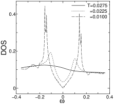
Figure 1: Temperature dependence of the DOS given by the FLEX approximation for YBCO ($n=0.9$). Note that $T_{\rm c}=0.024$.

In the FLEX approximation, the normal and anomalous self-energies are given by

$$\Sigma^{n}(\mathbf{k},i{\epsilon}_{n}) = \displaystyle\frac{{\rm U}^{2}T}{N}\sum_{\mathbf{k},l}G_{\mathbf{q+k}}(i{\epsilon}_{n}+i\omega_{l})$$ (2)

$$\times\displaystyle\left(\frac{3}{2}\chi_{s}+\frac{1}{2}\chi_{c}-\chi_{0}\right)_{\mathbf{q},\omega_{l}}$$

$$\Sigma^{a}(\mathbf{k},i{\epsilon}_{n}) = \displaystyle\frac{-{\rm U}^{2}T}{N}\sum_{\mathbf{k},l}F^{\dagger}_{\mathbf{q+k}}(i{\epsilon}_{n}+i\omega_{l})$$ (3)

$$\times\displaystyle\left(\frac{3}{2}\chi_{s}-\frac{1}{2}\chi_{c}-\phi_{0}\right)_{\mathbf{q},\omega_{l}}$$

where ${\epsilon}_{n}=\pi T(2n+1)$ and ${\omega}_{l}=2\pi Tl$ are the Matsubara frequencies for fermions and bosons, respectively. $\chi_{s}$ and $\chi_{c}$ are the dynamical spin and charge susceptibilities, which are given by

$$\chi_{s}(\mathbf{q},i\omega_{l})=\displaystyle\frac{\chi_{0}+\phi_{0}}{1-{\rm U}(\chi_{0}+\phi_{0})}$$ (4)

$$\chi_{c}(\mathbf{q},i\omega_{l})=\displaystyle\frac{\chi_{0}-\phi_{0}}{1-{\rm U}(\chi_{0}-\phi_{0})}$$ (5)

$$\chi_{0}(\mathbf{q},i\omega_{l})=-\displaystyle\frac{T}{N}\sum_{\mathbf{k},n}G_{\mathbf{k+q}}(i{\epsilon}_{n}+i\omega_{l})G_{\mathbf{k}}(i{\epsilon}_{n})$$ (6)

$$\phi_{0}(\mathbf{q},i\omega_{l})=-\displaystyle\frac{T}{N}\sum_{\mathbf{k},n}F^{\dagger}_{\mathbf{k+q}}(i{\epsilon}_{n}+i\omega_{l})F_{\mathbf{k}}(i{\epsilon}_{n})$$ (7)

where $G$ and $F$ are the normal and anomalous Green function, respectively. They are given by

$$G(i{\epsilon}_{n}) = (i{\epsilon}_{n}+{\tilde{\epsilon}}_{\mathbf{k}}+\Sigma^{n}(-i{\epsilon}_{n}))D({\epsilon}_{n})^{-1}$$ (8)

$$F(i{\epsilon}_{n}) = \Sigma^{a}(-i{\epsilon}_{n})D(i{\epsilon}_{n})^{-1}$$ (9)

$$D(i{\epsilon}_{n}) = (-{\epsilon}_{n}-{\tilde{\epsilon}}_{\mathbf{k}}+\Sigma^{n}(-i{\epsilon}_{n}))(-{\epsilon}_{n}+{\tilde{\epsilon}}_{\mathbf{k}}+\Sigma^{n}(i{\epsilon}_{n}))$$ (10)

$$-(\Sigma^{a}(-i{\epsilon}_{n}))^{2}$$

where ${\tilde{\epsilon}}_{\mathbf{k}}={\epsilon}_{\mathbf{k}}-\mu$; $\mu$ is the chemical potential. In the FLEX approximation, we solve eqs. (2)-(10) self-consistently by choosing $\mu$ to adjust the electron filling $n$. In the following numerical study, we use $64\times 64$ ${{\bf k}}$-meshes and 2048 Matsubara frequencies. Figure 1 represents the density of states (DOS); $\rho({\omega})=\frac{1}{N}\sum_{{\bf k}}G_{{\bf k}}^{A}({\omega})/\pi$. Here, the advanced (retarded) Green function $G_{{\bf k}}^{A}({\omega})$ ($G_{{\bf k}}^{R}({\omega})$) is given by the numerical analytic continuation of the Matsubara Green function from the lower (upper) half plane in the complex ${\omega}$ space.

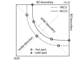
Figure 2: Position of the hot/cold spots for YBCO ($n=0.9$) and for NCCO ($n=1.10$). AFBZ represents the antiferromagnetic Brillouin zone.

Figure 2 shows the location of the hot/cold spots for both YBCO and NCCO in the normal state. The transport phenomena are governed by QPs around the cold spot, where the QP damping rate $\gamma_{{\bf k}}={\rm Im}\Sigma_{{\bf k}}^{n}(-i\delta)$ [$=1/2\tau_{{\bf k}}$] takes the minimum value. According to the FLEX approximation, the cold-spot in hole-doped [electron-doped] systems is around $(\pi/2,\pi/2)$ [$(\pi,0)$] Kontani-Hall . The position of the cold-spot in electron-doped systems was confirmed by ARPES measurements Armitage1 ; Armitage2 after the theoretical prediction Kontani-Hall .

Hereafter, we derive the electric thermal conductivity $\kappa$. According to the linear response theory Lee ; Jujo ; Kontani-nu ,

$$\kappa=\displaystyle\frac{-1}{T}\int^{\beta}_{0}d\tau\sum_{k_{1},k_{2}}\frac{1}{i\omega}\langle Q_{k_{1}}(\tau)Q_{k_{2}}(0)\rangle e^{i\omega\tau}\mid_{\omega\rightarrow 0}$$ (11)

$$\hat{Q}_{\mathbf{k}x}(\tau)=\hat{q}_{\mathbf{k}x\uparrow}+\hat{q}_{\mathbf{k}x\downarrow}+\hat{q}^{a}_{\mathbf{k}x}+\hat{q}^{a\dagger}_{\mathbf{k}x}$$ (12)

where $\hat{Q}_{\mathbf{k}x}$ is the heat current operator in the superconducting state: $\hat{q}_{\mathbf{k}x\sigma}$ and $\hat{q}^{a}_{\mathbf{k}x}$ are given by

$$\hat{q}_{\mathbf{k}x\sigma}= \omega\hat{v}_{\mathbf{k}x\sigma},\ \ \ \hat{q}^{a}_{\mathbf{k}x}= \omega\hat{v}_{\mathbf{k}x},$$ (13)

where $\hat{v}_{\mathbf{k}x\sigma}$ represents the “Fermi velocity” and $\hat{v}^{a}_{\mathbf{k}x}$ is the “gap velocity” Lee :

$$\hat{v}_{\mathbf{k}x\sigma}= v_{\mathbf{k}x}c^{\dagger}_{\mathbf{k}\sigma}c_{\mathbf{k}\sigma},\ \ \ \hat{v}^{a}_{\mathbf{k}x}= v_{\mathbf{k}x}^{a}c^{\dagger}_{\mathbf{k}\uparrow}c^{\dagger}_{-\mathbf{k}\downarrow},$$ (14)

where $v_{\mathbf{k}x}=v_{\mathbf{k}x}^{0}+\displaystyle\frac{\partial\Sigma^{n}_{\mathbf{k}}}{\partial k_{x}}$ and $v_{\mathbf{k}x}^{a}=\displaystyle\frac{\partial\Sigma^{a}_{\mathbf{k}}}{\partial k_{x}}$.

As a result, the expression for $\kappa$ in the SC state with dropping the current vertex correction (CVC) is given by Lee ; Jujo ; Kontani-nu

$$\kappa = \displaystyle\frac{1}{2T}\sum_{\mathbf{k}}\int dz\left(-\frac{\partial f(z)}{\partial z}\right)\{2q_{\mathbf{k}x}^{2}(G^{R}_{\mathbf{k}}(z)G^{A}_{k}(z)$$ (15)

$$- F^{R}_{\mathbf{k}}(z)F^{A}_{\mathbf{k}}(z))$$

$$+ q^{a2}_{\mathbf{k}x}(-G^{R}_{\mathbf{k}}(-z)G^{R}_{\mathbf{k}}(z)-G^{A}_{\mathbf{k}}(-z)G^{A}_{\mathbf{k}}(z)$$

$$+ 2F^{R}_{\mathbf{k}}(z)F^{A}_{\mathbf{k}}(z))$$

$$+ 4q_{\mathbf{k}x}q^{a}_{\mathbf{k}x}(-G^{R}_{\mathbf{k}}(z)F^{A}_{\mathbf{k}}(z)-F^{R}_{\mathbf{k}}(z)G^{A}_{\mathbf{k}}(z))\}$$

where $f(z)=(e^{z/T}+1)^{-1}$. In the normal state, heat CVC due to Coulomb interaction is small, as shown in the second-order perturbation theory with respect to $U$ Kontani-nu , and in the FLEX approximation Kontani-nu-HTSC . This fact will also be true below $T_{c}$ since the particle-nonconserving four point vertex is much smaller than the particle-conserving one Leggett . Therefore, we neglect the heat CVC in the present numerical study. We find that the first term in eq. (15), which is proportional to $\{q_{\mathbf{k}x}\}^{2}$, is predominant, and the other terms which contain the gap velocity, $q_{\mathbf{k}x}^{a}$, are negligibly small. On the other hand, the charge CVC gives anomalous transport properties for $R_{\rm H}$ Kontani-Hall , $S$ Kontani-S , magnetoresistance Kontani-MR-HTSC and Nernst coefficient Kontani-nu-HTSC both in hole-doped and electron-doped systems. Anomalous transport phenomena due to charge CVC are also observed in CeMIn₅ (M=Co,Rh) Nakajima2 and in $\kappa$-(BEDT-TTF)₂X Taniguchi .

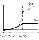
Figure 3: Schematic $T$-dependences of ${\gamma}_{{\bf k}}^{\rm FLEX}$ and $\gamma_{\rm imp}$.

Here, we include the QP damping due to impurity scattering ${\gamma}_{\rm imp}$ by replacing $\Sigma^{nR}(\mathbf{k},\omega)\rightarrow\Sigma^{nR}(\mathbf{k},\omega)-i\gamma_{\rm imp}$. Then, the total QP damping rate is ${\gamma}_{{\bf k}}={\gamma}_{{\bf k}}^{\rm FLEX}+\gamma_{\rm imp}$ Hirshfeld ; Lofwander , where ${\gamma}_{{\bf k}}^{\rm FLEX}={\rm Im}\Sigma^{nR}(\mathbf{k},\omega)$. In the $t$-matrix approximation, $\gamma_{\rm imp}=n_{\rm imp}{\rm Im}\{-1/(I^{-1}-g_{0})\}|_{{\omega}=0}$, where $n_{\rm imp}$ is the impurity concentration, $I$ is the impurity potential, and $g_{0}\equiv\frac{1}{N}\sum_{{\bf k}}G^{R}_{\mathbf{k}}$ is the local Green function. Hereafter, we consider the nearly unitary limit case $I\sim\infty$ where $\gamma_{\rm imp}(T=0)$ takes a constant value in the self-consistent calculation Hirshfeld ; Lofwander , and assume that $\gamma_{\rm imp}\ll\gamma_{{\bf k}}$ at $T=T_{\rm c}$. In this case, we are allowed to put $\gamma_{\rm imp}(T)=\gamma_{\rm imp}(T=0)$ since the $T$-dependence of $\gamma_{\rm imp}$ affects $\kappa$ near $T_{\rm c}$ only slightly. A schematic $T$-dependences of ${\gamma}_{{\bf k}}^{\rm FLEX}$ and $\gamma_{\rm imp}$ are shown in Fig. 3.

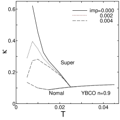
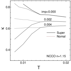
Figure 4: Obtained $\kappa$ for YBCO ($n=0.9$; $T_{\rm c}=0.024$) and for NCCO ($n=1.15$; $T_{\rm c}=0.014$), for $\gamma_{\rm imp}=0$, 0.002 and 0.004. “Normal” represents $\kappa$ given by the normal state FLEX approximation under the constraint $F=\Sigma^{a}=0$.

Figure 4 represents the temperature-dependence of $\kappa$ given by eq. (15). In YBCO, $\kappa$ increases drastically below $T_{\rm c}$ since the AF fluctuations, which are the origin of inelastic scattering, are reduced due to the SC gap. Since $\gamma_{{\bf k}}$ is much larger than $\gamma_{\rm imp}$ at $T>T_{\rm c}$, $\kappa$ in the normal state is affected by $\gamma_{\rm imp}$ only slightly. For $T\ll T_{\rm c}$, on the other hand, $\kappa$ is suppressed by $\gamma_{\rm imp}$; $\kappa$ shows the maximum when $\gamma_{{\bf k}}^{\rm FLEX}\sim{\gamma}_{\rm imp}$ is satisfied at the nodal point. The obtained result is consistent with experiments Popoviciu ; Ong ; Ong2 . In strong contrast, in NCCO, “coherence peak” in $\kappa$ is very small even for ${\gamma}_{\rm imp}=0$, which is also consistent with experiments Cohn ; Fujishiro .

Here, we discuss the reason why the coherence peak in $\kappa$ is present in YBCO whereas it is absent in NCCO. Below $T_{\rm c}$, only thermally excited QPs above the SC gap can contribute to $\kappa$, except at the nodal point. According to eq. (15), thermal conductivities in the normal state ($\kappa_{n}$) and in the line-node SC state ($\kappa_{s}$), where $\rho({\epsilon})\propto|{\epsilon}|$, are approximately given by

$$\kappa_{n}\propto T/\gamma_{\rm cold}$$ (16)

$$\kappa_{s}\propto T^{2}/\gamma_{\rm node}$$ (17)

where $\gamma_{\rm cold}$ and $\gamma_{\rm node}$ represent $\gamma_{{\bf k}}$ at the cold spot above $T_{\rm c}$ and that at the nodal point below $T_{\rm c}$, respectively.

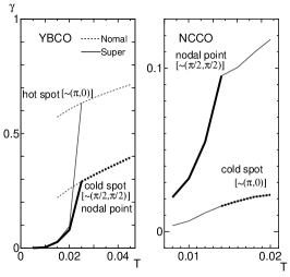
Figure 5: $T$-dependence of $\gamma_{{\bf k}}$ for both YBCO and NCCO for $\gamma_{\rm imp}=0$. Thick full lines and thick broken lines represent $\gamma_{\rm node}$ ($T<T_{\rm c}$) and $\gamma_{\rm cold}$ ($T>T_{\rm c}$), respectively.

Figure 5 shows the $T$-dependence of $\gamma_{{\bf k}}$ given by the FLEX approximation. In YBCO, both $\gamma_{\rm cold}$ and $\gamma_{\rm node}$ are given by $\gamma_{{\bf k}}$ at the same point; ${{\bf k}}\approx(\pi/2,\pi/2)$. As the temperature drops, $\gamma_{\rm cold}$ decreases moderately in proportion to $T$ in the normal state. Below $T_{\rm c}$, $\gamma_{\rm node}$ quickly approaches zero since inelastic scattering is suppressed by the SC gap. As a result, $\kappa$ shows a prominent coherence peak below $T_{\rm c}$, as recognized by eqs. (16) and (17). In NCCO, on the other hand, $\gamma_{\rm cold}$ is given by $\gamma_{{\bf k}}$ at ${{\bf k}}\approx(\pi,0)$, which is different from the nodal point of the SC gap; ${{\bf k}}\approx(\pi/2,\pi/2)$. Since $\gamma_{\rm node}$ is much larger than $\gamma_{\rm cold}$ at $T=T_{\rm c}$ in NCCO as shown in Fig. 5, $\kappa$ is not enhanced in NCCO below $T_{\rm c}$. Although the numerical accuracy becomes worse for NCCO below $T\sim 0.015$, the obtained result of $\kappa$ will be qualitatively reliable. In summary, the coherence peak in $\kappa$ is absent even in nodal SC when the cold spot and the nodal point are different.

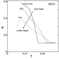
Figure 6: $n$-dependence of $\kappa$ for YBCO; $n=0.8\sim 0.9$.

Figure 6 shows the obtained doping dependence of $\kappa$ in YBCO. In over-doped case ($n=0.8$), the enhancement of $\kappa$ is largest, and it decreases in optimally ($n=0.85$) and under-doped ($n=0.9$) cases since the cold spot approaches the AFBZ as $n\rightarrow 1$. This tendency is consistent with experiments Popoviciu . Note that in real materials, $T_{\rm c}$ in under-doped case is smaller than that in optically-doped case. In the FLEX approximation, however, $T_{\rm c}$ monotonically increases as $n\rightarrow 1$ since the pseudo-gap state in under-doped region cannot be described. The characteristic pseudo-gap phenomena are well described by including the self-energy correction due to strong SC fluctuations into the FLEX approximation, which is called the FLEX+$T$-matrix approximation Yamada-text ; Kontani-nu-HTSC .

In the present work, we assumed that the inelastic scattering is dominant, and neglected the temperature dependence of ${\gamma}_{\rm imp}$. This assumption will be allowed for clean optimally-doped HTSCs. In dirty samples where elastic scattering is large, we should calculate the $T$-dependence of ${\gamma}_{\rm imp}$ using the self-consistent $t$-matrix approximation Hirshfeld ; Lofwander . In under-doped systems, however, the $t$-matrix approximation is not sufficient since the radius of “effective impurity potential” is enlarged due to electron-electron correlation, which can be described by the $GV^{I}$-method in Ref. GVI . For a reliable study of $\kappa$ in under-doped systems, it will be necessary to take account of residual disorders using the $GV^{I}$-method.

In summary, we studied thermal conductivity $\kappa$ in HTSCs. In the hole-doped case, $\kappa$ shows a prominent “coherence peak” below $T_{\rm c}$, whereas it is absent in the electron-doped case. Based on the FLEX approximation, such a contrasting behavior of $\kappa$ is well explained, although both YBCO and NCCO are pure $d_{x^{2}\mbox{-}y^{2}}$-wave superconductors. We do not have to assume a full-gap state in NCCO (such as $d+is$) to explain the absence of a coherence peak, which originates from the fact that the cold spot (line) in the normal state [$\sim(\pi,0)$] is not on the nodal point (line) of the SC gap. The present study will open the way for the theoretical study of $\kappa$ in various interesting unconventional superconductors.

The authors acknowledge fruitful discussions with Y. Matsuda and K. Izawa. This work was supported by Grant-in-Aid from MEXT. Numerical calculations were performed at the supercomputer center, ISSP.

References

- (1) J. Takeda, T. Nishikawa, and M. Sato: Physica C 231 (1994) 293.
- (2) H. Kontani, K. Kanki and K. Ueda: Phys. Rev. B 59 (1999) 14723.
- (3) H. Kontani: J. Phys. Soc. Jpn. 70 (2001) 2840.
- (4) H. Kontani and K. Yamada: J. Phy. Soc. Jpn. 74 (2005) 155.
- (5) K. Izawa, H. Yamaguchi, Y. Matsuda, H. Shishido, R. Settai and Y. Onuki: Phys. Rev. Lett. 87 (2001) 057002.
- (6) Y. Matsuda, K. Izawa and I. Vekhter, J. Phys.: Condens. Matter 18 (2006) R705.
- (7) C.P. Popoviciu and J.L. Cohn: Phys. Rev. B 55 (1997) 3155.
- (8) K. Krishana, J. M. Harris, and N. P. Ong: Phys. Rev. Lett. 75 (1995) 3529
- (9) Y. Zhang, N. P. Ong, P. W. Anderson, D. A. Bonn, R. Liang, and W. N. Hardy: Phys. Rev. Lett. 86 (2001) 890.
- (10) R. Movshovich, M. Jaime, J.D. Thompson1, C. Petrovic, Z. Fisk, P.G. Pagliuso, and J.L. Sarrao: Phys. Rev. Lett. 86 (2001) 5152.
- (11) Y. Kasahara, Y. Nakajima, K. Izawa, Y. Matsuda, K. Behnia, H. Shishido, R. Settai, and Y. Onuki: Phys. Rev. B 72 (2005) 214515.
- (12) Y. Matsuda et al, preprint.
- (13) P.J. Hirshfeld and W.O. Putikka: Phys. Rev. Lett. 77 (1996) 3909.
- (14) J. L. Cohn, M.S. Osofsky, J.L. Peng, Z. Y. Li, and R.L. Greene: Phys. Rev. B 46 (1992) 12053.
- (15) H. Fujishiro, M. Ikeba, M. Yagi, M. Matsukawa, H. Ogasawara and K. Noto: Physica B 219&220 (1996) 163.
- (16) H. Matsui, K. Terashima, T. Sato, T. Takahashi, M. Fujita, and K. Yamada: Phys. Rev. Lett. 95 (2005) 017003.
- (17) H. Yoshimura and D.S. Hirashima: J. Phys. Soc. Jpn 73 (2004) 2057.
- (18) M.M. Qazilbash, A. Biswas, Y. Dagan, R.A. Ott, and R.L. Greene: Phys. Rev. B 68 (2003) 024502.
- (19) N.P. Armitage, D.H. Lu, C. Kim, A. Damascelli, K.M. Shen, F. Ronning, D.L. Feng, P. Bogdanov, and Z.-X. Shen: Phys. Rev. Lett. 87 (2001) 147003.
- (20) N. P. Armitage, F. Ronning, D. H. Lu, C. Kim, A. Damascelli, K. M. Shen, D. L. Feng, H. Eisaki, Z.-X. Shen, P. K. Mang, N. Kaneko, M. Greven, Y. Onose, Y. Taguchi, and Y. Tokura: Phys. Rev. Lett. 88, 257001 (2002).
- (21) A.C. Durst and P.A. Lee: Phys. Rev. B 62 (2000) 1270.
- (22) T. Jujo: J. Phy. Soc. Jpn. 70 (2000) 1349.
- (23) H. Kontani, J. Phys. Rev. B 67 (2003) 014408.
- (24) H. Kontani: Phys. Soc. Jpn. 70 (2001) 1873.
- (25) H. Kontani, Phys. Rev. Lett. 89 (2002) 237003.
- (26) A.J. Leggett: Phys. Rev. 146 (1965) A1869.
- (27) Y. Nakajima, H. Shishido, H. Nakai, T. Shibauchi, K. Behnia, K. Izawa, M. Hedo, Y. Uwatoko, T. Matsumoto, R. Settai, Y. Onuki, H. Kontani, and Y. Matsuda: J. Phys. Soc. Jpn. 76 (2007) 027403.
- (28) K. Katayama, T. Nagai, H. Taniguchi, K. Satoh, N. Tajima and R. Kato, to be published in J. Low Temp. Phys. (2006).
- (29) T. Lofwander and M. Fogelstrom: Phys. Rev. Lett. 95 (2005) 107006.
- (30) K. Yamada: Electron Correlation in Metals (Cambridge Univ. Press 2004).
- (31) H. Kontani and M. Ohno: Phys. Rev. B 74, 014406 (2006).