Recovering Multiplexing Loss Through Successive Relaying Using Repetition Coding

Abstract

In this paper, a transmission protocol is studied for a two relay wireless network in which simple repetition coding is applied at the relays. Information-theoretic achievable rates for this transmission scheme are given, and a space-time V-BLAST signalling and detection method that can approach them is developed. It is shown through the diversity multiplexing tradeoff analysis that this transmission scheme can recover the multiplexing loss of the half-duplex relay network, while retaining some diversity gain. This scheme is also compared with conventional transmission protocols that exploit only the diversity of the network at the cost of a multiplexing loss. It is shown that the new transmission protocol offers significant performance advantages over conventional protocols, especially when the interference between the two relays is sufficiently strong.

I Introduction

I-A Background

In the past few years, cooperative diversity protocols [1, 2, 3, 4, 8, 9, 10, 12, 7, 11] have been studied intensively to improve the diversity of relay networks. In most of the prior work, a time-division-multiple-access (TDMA) half-duplex transmission is assumed and the most popular transmission protocol (e.g.[2]) can be described in two steps: In the first step, the source broadcasts the information to all the relays. The relays process the information and forward it to the destination (in either the same or a different time slot) in the second step, while the source remains silent. The destination performs decoding based on the message it received in both steps. We refer to this protocol as the classic protocol throughout the paper.

For digital relaying, where the relay decodes, re-encodes and forwards the message, the simplest coding method is repetition coding[2, 3], where the source and all the relays use the same codebook. This scheme can achieve full diversity and is also practically implementable. Any capacity achieving AWGN channel codes can be used to approach the performance limit of such schemes. The disadvantage of this scheme is that it requires the relays to transmit in orthogonal time slots in the second step in order for the destination to combine effectively the relays’ signals. This will result in a significant multiplexing loss compared with direct transmission. Space-time codes, which were originally applied in multiple-input multiple-output (MIMO) systems, have been suggested for use in relay networks (e.g. [3, 24]). Here all the relays can transmit the signals simultaneously to the destination in the second step and the multiplexing factor is recovered to $1/2$. However, this still causes spectral inefficiency for the high signal to noise ratio (SNR) region. In fact, the network capacity in this scenario will become only half of the non-relay network capacity for high SNR, even assuming that the message is always correctly decoded at the relays.

To fully recover the multiplexing loss, much more complicated protocols and coding strategies have been proposed in [9], where new independent random codebooks are used at the relays to transmit the same information as they received from the source, while the relays can adjust their listening times dynamically in the first step. Those approaches, which are based on Shannon’s random coding theory, are currently theoretical and extremely difficult to realize in reality. Practical coding design for relay networks often follows a quite different approach from these theoretical investigations (see [25, 26, 27, 28] for example).

Instead of using complicated coding schemes, a protocol using repetition coded relaying was proposed in [4](see also [29]) to avoid multiplexing loss for single relay channels. In this protocol, denoted as protocol I in [4], the source transmits a different message in the second time slot, so that the destination sees a collision of messages from both the relay and the source in the second time slot. Although multiplexing loss is recovered due to the continuous transmission of the source, diversity gain is lost due to the fact that the source transmission in time slot two is not relayed to the destination.

I-B Contribution of the Paper

In this paper, we study a transmission protocol based on protocol I in [4] for digital relaying. By adding an additional relay in the network and making the two relays transmit in turn, we show that multiplexing loss can be effectively recovered while diversity/combining gain can still be obtained. Specifically, $L$ codewords can be transmitted in $(L+1)$ time slots with joint decoding at the destination. Our analysis is based on two different scenarios: (a) The instantaneous channel state information (CSI) is known to the receiver and can be fed back to the transmitter; (b) The instantaneous CSI is known to the receiver but is not available to the transmitter. We make the following observations in this paper for the proposed protocol:

• For scenario (a), we derive the achievable rates for this protocol when repetition coding is assumed to be used at the relays. We show that in certain scenarios, the capacity for the network becomes that for a MIMO system with $L$ inputs and $L+1$ outputs and has a multiplexing gain of $L/(L+1)$. Assuming that the relays correctly decode the signal, we show that the proposed protocol offers significant capacity performance advantages over the classic protocol due to its improved multiplexing gain.

• We also discuss the source-relay channel conditions and the interference that arises between the relays. We derive the required channel constraints for the optimal performance of such a protocol as a function of SNR, as well as the achievable rates for different channel conditions. We believe these analyses offer strong insights for adaptive protocol design, where relaying and direct transmission can be combined. Based on our network models we show that the proposed protocol, combined with the direct transmission protocol, can also give a significant capacity performance advantage over the classic protocol, especially when the two relays are located close to each other.

• We propose a practical low-rate feedback V-BLAST decoding algorithm which approaches the theoretical achievable rates for a slow fading environment.

• For scenario (b), we analyze the diversity multiplexing tradeoff for such a network when $L$ is large, conditioned on the signals being correctly decoded at the relays. We show that in this scenario the network mimics a multiple-input single-output (MISO) system with two transmit and one receive antennas. This means it can offer a maximal diversity gain of two with almost no multiplexing loss.

I-C Relations to Previous and Concurrent Work

The idea for successive relaying first appeared in [30]. This study was focused on amplify-and-forward relaying and did not offer insight into the achievable rates and diversity multiplexing tradeoff for such relaying methods. The scheme has been further analyzed for amplify-and-forward relaying in [6, 31] and [32]. In [6] capacity analysis was performed assuming that the direct link is ignored. Hence no diversity can be obtained at the destination. The analysis in very recent papers [31] and [32] make the assumption that the relays are isolated, when there are more than one relay. Also the relay-to-relay link in [31] and [32] acts in a different way from that in our work due to a different relaying mode.

A further work [5] also analyzes the capacity for such schemes when digital relaying is used. One major difference between [5] and our work is that the direct link is ignored in [5] while it is considered in this paper. Therefore the analysis becomes different for the following reasons. First, the scheme in [5] does not offer any cooperative diversity gain, which is a very important benefit that the relay can offer. We will show in this paper that a diversity gain of 2 can be obtained by considering the direct link. Secondly, this also results in very different characteristics in terms of achievable rates and signalling methods due to the additional interference and diversity that the direct link introduces. In this paper we specifically analyze the network capacity under different channel and interference constraints, which were not given in [5]. Also the use of the V-BLAST decoder is unique to our paper. Finally, we note that the capacity analysis discussed in our paper in fact contains the scenario in [5] as a special case, i.e. the same capacity values as in [5] is obtained on assuming that the channel coefficient for the direct link is zero in our model. Therefore our analysis is more general, and the adaptive protocols introduced here fit better in the context of previous work on this topic [2].

II Protocol Design

We assume a four-node network model, where one source, one destination and two relays exist in the network. For simplicity, we denote the source as $S$, the destination as $D$, and the two relays as $R1$ and $R2$. We split the source transmission into different frames, each containing $L$ codewords denoted as $s_{l}$. These $L$ codewords are transmitted continuously by the source, and are decoded and forwarded by two relays successively in turn. Before decoding $L$ codewords, the destination waits for $L+1$ transmission time slots until all $L$ codewords are received, from both direct link and the relay links. It then performs joint decoding of all $L$ codewords. The specific steps for each transmission (reception) time slot for every frame are described as follows:

Time slot 1: $S$ transmits $s_{1}$. $R1$ listens to $s_{1}$ from $S$. $R2$ remains silent. $D$ receives $s_{1}$.

Time slot 2: $S$ transmits $s_{2}$. $R1$ decodes, re-encodes and forwards $s_{1}$. $R2$ listens to $s_{2}$ from $S$ while being interfered with by $s_{1}$ from $R1$. $D$ receives $s_{1}$ from $R1$ and $s_{2}$ from $S$.

Time slot 3: $S$ transmits $s_{3}$. $R2$ decodes, re-encodes and forwards $s_{2}$. $R1$ listens to $s_{3}$ from $S$ while being interfered with by $s_{2}$ from $R2$. $D$ receives $s_{2}$ from $R2$ and $s_{3}$ from $S$. The progress repeats until Time slot L.

Time slot L+1: $R1$ (or $R2$) decodes, re-encodes and forwards $s_{L}$. $D$ performs a joint decoding algorithm to decode all $L$ codewords received from the $L+1$ transmission time slots.

The transmission schedule for the first three time slots for each frame is shown in Fig. 1. Compared with direct transmission, the multiplexing ratio for this protocol is clearly $L/(L+1)$, which approaches 1 for large frame lengths $L$. Unlike protocol III in [4], the destination always receives two copies of each codeword, from both the direct and relay link (a delayed version). This implies that diversity gain can still be realized by this protocol.

The major issue for this protocol to be effectively implemented is to tackle the co-channel interference at the relays and the destination. As described above, except for the first and last time slot, the relays and the destination always observe collisions from different transmitters (i.e. the source or the relays). Suppression of the interference thus becomes a major problem. We will discuss this problem further in the next two sections.

III Achievable Rates

When the channel information can be fed back to the transmitter, one can implement adaptive coding and modulation to achieve the system performance limit. Thus capacity is a key measurement in this scenario. We assume a slow, flat, block fading environment, where the channel remains static for each message frame transmission (i.e. $L+1$ time slots). Note that while this assumption is made for presentation simplicity, the capacity analysis can also be applied to a more relaxed flat block fading scenario, e.g. fast fading where each channel coefficient changes for each time slot. We also assume that each transmitter transmits with equal power (i.e. no power allocation or saving among the source and relays). We denote the channel coefficient between node $a$ and $b$ by $h_{a,b}$, which may contain path-loss, Rayleigh fading, and lognormal shadowing. For simplicity, we denote the capacity function $\log_{2}\left({1+x}\right)$ by $C\left(x\right)$, in which the parameter $SNR$ denotes the ratio of signal power to the noise variance at the receiver.

III-A Source-Relay Link

In order for the relays to decode the signals correctly, the source transmission rate should be below the Shannon capacity of the source-relay channels. We express this constraint as

$$R_{i}\leq C\left({\left|{h_{S,r_{i}}}\right|^{2}SNR}\right),1\leq i\leq L$$ (1)

where $r_{i}$ is the $i$th element in the $L$ dimensional relay index vector

$${\bf{r}}={\left[{\begin{array}[]{*{20}c}{R1}&{R2}&{R1}&{R2}&{R1}\cdots\\ \end{array}}\right]},$$ (2)

and $R_{i}$ denotes the achievable rate for $s_{i}$.

III-B Interference Cancellation Between Relays

One major defect of the protocol is the interference generated among the relays when one relay is listening to the message from the source, while the other relay is transmitting the message to the destination. This situation mimics a two user Gaussian interference channel [13], where two transmitters (the source and one of the relays) are transmitting messages each intended for one of the two receivers (the other relay and the destination). The optimal solution for this problem is still open. We concern ourselves only with suppressing the interference at the relays at this stage (interference suppression at the destination will be left until all $L$ signals are transmitted). We give a very simple decoding criterion for the relays: if the interference between relays is stronger than the desired signal, we decode the interference and subtract it from the received signals before decoding the desired signal. Otherwise, we decode the signal directly while treating the interference as Gaussian noise.

The achievable rate is therefore based on different channel conditions between the source to relay and the relay to destination links. For example, when $R1$ transmits $s_{1}$ while $R2$ is receiving $s_{2}$, if $\left|{h_{R1,R2}}\right|\succ\left|{h_{S,R2}}\right|$, $R2$ first decodes $s_{1}$, subtracts it (as the interference), then decodes $s_{2}$ (as the desired signal). Therefore, besides the rate constraint proposed in the previous subsection, there will be an additional rate constraint for $s_{1}$ to be correctly decoded at $R2$, which can be expressed as follows:

$$R_{1}\leq C\left({\frac{{\left|{h_{R1,R2}}\right|^{2}SNR}}{{1+\left|{h_{S,R2}}\right|^{2}SNR}}}\right).$$ (3)

Otherwise if $s_{2}$ is decoded directly, treating $s_{1}$ as noise, the achievable rate for $s_{2}$ is further constrained and can be expressed as

$$R_{2}\leq C\left({\frac{{\left|{h_{S,R2}}\right|^{2}SNR}}{{1+\left|{h_{R1,R2}}\right|^{2}SNR}}}\right).$$ (4)

Note that this decoding criterion applies from the second time slot to the $L$th time slot when transmitting each frame. In slot $i$, inequality (3) can be adapted to a constraint on $R_{i-1}$ and inequality (4) can be adapted to a constraint on $R_{i}$.

III-C Space-Time Processing at the Destination

If the transmission rate is below the Shannon capacity proposed by the previous two subsections, the relays can successfully decode and retransmit the signals for all the $L+1$ time slots. The input output channel relation for the relay network is equivalent to a multiple access MIMO channel, which can be expressed as

$${\bf{y}}=\sqrt{SNR}\underbrace{\left[{\begin{array}[]{*{20}c}{h_{S,D}}&0&0&0&0\\ {h_{r_{1},D}}&{h_{S,D}}&0&0&0\\ 0&{h_{r_{2},D}}&{h_{S,D}}&0&0\\ 0&0&\ddots&\ddots&0\\ 0&0&0&{h_{r_{L-1},D}}&{h_{S,D}}\\ 0&0&0&0&{h_{r_{L},D}}\\ \end{array}}\right]}_{\bf{H}}{\bf{s}}+{\bf{n}},$$ (5)

where $\bf{y}$ is the $(L+1)\times 1$ received signal vector, $\bf{s}$ is the $L\times 1$ transmitted signal vector and ${\bf{n}}$ is an $(L+1)\times 1$ complex circular additive white Gaussian noise vector at the destination. Unlike conventional multiple access MIMO channels, the dimensions of $\bf{y}$, $\bf{s}$ and ${\bf{n}}$ are expanded in the time domain rather than the space domain. However, the capacity region should be the same, which can be expressed as follows [14]:

$$R_{k} \leq \log_{2}\left({\det\left({{\bf{I}}+{\bf{h}}_{k}{\bf{h}}_{k}^{H}SNR}\right)}\right),$$ (6)

$$R_{k_{1}}+R_{k_{2}} \leq \log_{2}\left({\det\left({{\bf{I}}+SNR\left({{\bf{h}}_{k_{1}}{\bf{h}}_{k_{1}}^{H}+{\bf{h}}_{k_{2}}{\bf{h}}_{k_{2}}^{H}}\right)}\right)}\right),$$

$$...$$

$$\sum\limits_{k=1}^{L}{R_{k}} \leq \log_{2}\left({\det\left({{\bf{I}}+{\bf{HH}}^{H}SNR}\right)}\right),$$ (8)

where ${\bf{h}}_{k}$ denotes the $k$th column of $\bf{H}$. As it is extremely complicated to give an exact description for the rate region of each signal when $L>2$, we will concentrate only on inequalities (6) and (8) to give a sum capacity upper bound for the network in the next subsection. However, as will be shown later in the paper, this bound is extremely tight and is achievable when a space-time V-BLAST algorithm is applied at the destination to decode the signals in a slow fading scenario.

III-D Network Achievable Rates

Combining the transmission rate constraints proposed by the previous three subsections, we provide a way of calculating the network capacity upper bound for the proposed protocol. First, we impose a rate constraint $R_{i}$ for each transmitted codeword $s_{i}$. In the first time slot (initialization), we write

$$R_{S,r_{1}}\leq C\left({\left|{h_{S,r_{1}}}\right|^{2}SNR}\right).$$ (9)

For $(i+1)$th time slot (for $1\leq i\leq L-1$), we calculate the rate constraints based on the decoding criterion at the relays. The calculation can be written as a logical if statement as follows:

if $h_{R1,R2}\succ h_{S,r_{i+1}}$,

$$R_{i}\leq\min\left({C\left({\frac{{\left|{h_{R1,R2}}\right|^{2}SNR}}{{1+\left|{h_{S,r_{i+1}}}\right|^{2}SNR}}}\right),R_{S,r_{i}},C\left({\left|{h_{S,D}}\right|^{2}SNR+\left|{h_{r_{i},D}}\right|^{2}}SNR\right)}\right),$$

$$R_{S,r_{i+1}}\leq C\left({\left|{h_{S,r_{i+1}}}\right|^{2}}SNR\right);$$ (10)

else

$$R_{i}\leq\min\left({R_{S,r_{i}},C\left({\left|{h_{S,D}}\right|^{2}SNR+\left|{h_{r_{i},D}}\right|^{2}SNR}\right)}\right),$$

$$R_{S,r_{i+1}}\leq C\left({\frac{{\left|{h_{S,r_{i+1}}}\right|^{2}SNR}}{{1+\left|{h_{R1,R2}}\right|^{2}SNR}}}\right);$$ (11)

end.

Note that the term $C\left({\left|{h_{S,D}}\right|^{2}SNR+\left|{h_{r_{i},D}}\right|^{2}SNR}\right)$ represents the constraint expressed by (6). The purpose of the if statement is to select the decoding order at the relay and to decide whether equation (3) or (4) is the correct constraint to apply.

In the $(L+1)$th time slot, we have

$$R_{L}\leq\min\left({R_{S,r_{L}},C\left({\left|{h_{S,D}}\right|^{2}SNR+\left|{h_{r_{L},D}}\right|^{2}SNR}\right)}\right).$$ (12)

Combining these constraints with the sum capacity constraint expressed by (8), an achievable rate per time slot can then be written as

$$C_{ach}=\frac{1}{L+1}\min\left(\mathop{\max}\limits_{R_{1}\cdots R_{L}}\left\{{\sum\limits_{i=1}^{L}{R_{i}}}\right\},\log_{2}\left({\det\left({{\bf{I}}+{\bf{HH}}^{H}SNR}\right)}\right)\right).$$ (13)

The first term in the $\min$ function comes from the calculation described above, the second one comes from equation (8).

III-E Interference Free Transmission

From the above discussion of the proposed protocol, it is clear that the interference between relays is one major and obvious factor that can significantly degrade the network capacity performance. However, it has been shown that for a Gaussian interference network, if the interference is sufficiently strong, the network can perform the same as an interference free network [15]. Specifically, for the scenario discussed in our model, if the interference between relays (i.e. the value of $\left|h_{R1,R2}\right|$) is so large that the following inequality holds

$$\frac{{\left|{h_{R1,R2}}\right|^{2}SNR}}{{1+\left|{h_{S,r_{i+1}}}\right|^{2}SNR}}\geq\min\left({\left|{h_{S,r_{i}}}\right|^{2}SNR,\left(\left|{h_{S,D}}\right|^{2}+\left|{h_{r_{i},D}}\right|^{2}\right)SNR}\right),i=1\cdots L,$$ (14)

then the relay can always correctly decode the interference and subtract it before decoding the desired message, without affecting the overall network capacity. In this situation, the capacity analysis for the $i$th ($1\leq i\leq L$) transmitted signal as expressed by (10)-(12) can be simplified to

$$R_{i}\leq\min\left(C\left({\left|{h_{S,r_{i}}}\right|^{2}SNR}\right),C\left({\left(\left|{h_{S,D}}\right|^{2}+\left|{h_{r_{i},D}}\right|^{2}\right)SNR}\right)\right).$$ (15)

It is obvious that the rate bounds provided by (15) are significantly larger than those provided by (10)-(12).

From the above capacity analysis, it can also be seen that the quality of the source to relay link (i.e. $h_{S,r_{i}}$) is also an important factor that may constrain the network capacity. This has also been justified and discussed in many papers (e.g. [2, 3, 7, 9, 12]). Similar to this previous work, we suggest that $h_{S,r_{i}}$ should be compared with $h_{S,D}$ or $h_{r_{i},D}$ before deciding to relay or not. For the interference free scenario discussed here, the constraint becomes

$$\left|{h_{S,r_{i}}}\right|^{2}\geq\left|{h_{S,D}}\right|^{2}+\left|{h_{r_{i},D}}\right|^{2},1\leq i\leq L.$$ (16)

The capacity expressed by (13) can be simplified to

$$C_{ach}=\frac{1}{L+1}\min\left({\sum\limits_{i=1}^{L}{C\left(\left({\left|{h_{S,D}}\right|^{2}+\left|{h_{r_{i},D}}\right|^{2}}\right)SNR\right)},\log_{2}\left({\det\left({{\bf{I}}+{\bf{HH}}^{H}SNR}\right)}\right)}\right).$$ (17)

By Jensen’s inequality [15] it is clear that

$$\sum\limits_{i=1}^{L}{C\left(\left({\left|{h_{S,D}}\right|^{2}+\left|{h_{r_{i},D}}\right|^{2}}\right)SNR\right)}\geq\log_{2}\left({\det\left({{\bf{I}}+{\bf{HH}}^{H}SNR}\right)}\right).$$ (18)

Therefore the rate is equal to the MIMO channel capacity equation with a multiplexing scaling factor:

$$C_{ach}=\frac{1}{L+1}\log_{2}\left({\det\left({{\bf{I}}+{\bf{HH}}^{H}SNR}\right)}\right).$$ (19)

This result shows that the proposed protocol can offer the best capacity performance conditioned on (14) and (16), which guarantees that the relays will correctly decode the message without affecting the network capacity. To summarize, we have the following theorem.

Theorem 1

Conditioned on (14) and (16), the capacity for the successive relaying scheme can be expressed as

$$C_{ach}=\frac{1}{L+1}\log_{2}\left({\det\left({{\bf{I}}+{\bf{HH}}^{H}SNR}\right)}\right)$$

where $\bf{H}$ denotes the channel matrix in (5).

It should be noted that this high interference scenario (i.e. condition (14)) is not uncommon in reality. A practical example is when the two relays (e.g. mobiles) are located close to each other. If the routing techniques are developed to choose these relays, the capacity performance can be significantly improved by applying the proposed protocol. To satisfy condition (16), an adaptive protocol can be developed from the proposed protocol to guarantee that the relays are used only when (16) holds, otherwise direct transmission is assumed. However, for a large dense network of relays, it is even not difficult to find two relays satisfying both (14) and (16). A simple example is a fixed relay network scenario [16], where the source to relay links are often assumed to be significantly better than the corresponding relay to destination links and the direct link. Therefore both (14) and (16) can be met by choosing the two nearby fixed relays. Furthermore, studies have shown that for a large relay network where many relays exist, choosing the best one or few relays will be preferable to using all the relays in many situations (e.g. [10, 17, 18, 20]). Therefore it is possible that the proposed relay protocol can be combined with relay selection techniques to achieve an even higher capacity gain over the classic multi-cast relay protocol, especially for high SNR conditions.

III-F The V-BLAST Algorithm

In this section we apply the low-rate feedback V-BLAST minimum mean squared error (MMSE) algorithm for detecting the signals at the destination. The V-BLAST algorithm was initially designed for spatial multiplexing MIMO systems [21]. For a system with $M$ transmit and $N$ receive antennas, the message at the transmitter is multiplexed into $M$ different signal streams, each independently encoded and transmitted to the receiver. The receiver uses $N$ antennas to detect and decode each signal stream by a V-BLAST MMSE detector [22]. The V-BLAST MMSE detection consists of $M$ iterations, each aimed at decoding one signal stream. For each iteration, the receiver applies the MMSE algorithm to detect and decode the strongest signal while treating the other signals as interference, then subtracts it from the received signal vector. The detection continues until all $M$ signal streams are decoded. The Shannon capacity of this system can be achieved if we assume that each signal is correctly decoded[23]:

$$C=\log_{2}\det\left({{\bf{I}}+{\bf{HH}}^{H}}SNR\right)=\sum\limits_{i=1}^{M}{\log_{2}}\left({1+SINR_{i}}\right),$$ (20)

where $SINR_{i}$ is the output signal to interference plus noise ratio (SINR) for signal $s_{i}$ in the V-BLAST detector. In order for each signal to be correctly decoded, a low-rate feedback channel can be used to feed the value of $SINR_{i}$ back to the transmitter. Adaptive modulation and coding should be applied to make the transmission rate for $s_{i}$ lower than ${\log_{2}}\left({1+SINR_{i}}\right)$.

Unlike traditional MIMO systems, when we apply this V-BLAST MMSE detector at the destination for the proposed protocol, each signal stream is independently encoded along the time dimension rather than the space dimension. When considering the rate bound $R_{i}$, the same analysis should be made as in Section III. The initialization step is the same as (9). For the $(i+1)$th time slot (for $1\leq i\leq L-1$), based on the same interference cancellation criterion as in Section III, the rate calculation can be performed as follows:

if $h_{R1,R2}\succ h_{S,r_{i+1}}$

$$R_{i}\leq\min\left({C\left({\frac{{\left|{h_{R1,R2}}\right|^{2}SNR}}{{1+\left|{h_{S,r_{i+1}}}\right|^{2}SNR}}}\right),R_{S,r_{i}},\log_{2}\left({1+SINR_{r_{i}}}\right)}\right),$$

$$R_{S,r_{i+1}}\leq C\left({\left|{h_{S,r_{i+1}}}\right|^{2}SNR}\right);$$ (21)

else

$$R_{i}\leq\min\left({R_{S,r_{i}},\log_{2}\left({1+SINR_{r_{i}}}\right)}\right),R_{S,r_{i+1}}\leq C\left({\frac{{\left|{h_{S,r_{i+1}}}\right|^{2}SNR}}{{1+\left|{h_{R1,R2}}\right|^{2}SNR}}}\right);$$ (22)

end.

In the $(L+1)$th time slot, we have

$$R_{L}\leq\min\left({R_{S,r_{L}},\log_{2}\left({1+SINR_{r_{L}}}\right)}\right).$$ (23)

The $SINR_{r_{i}}$ denotes the SINR for $s_{i}$, which is decoded, encoded and forwarded by relay $r_{i}$. The network capacity is therefore

$$C_{ach_{BLAST}}=\frac{1}{L+1}\mathop{\max}\limits_{R_{1}\cdots R_{L}}\left\{{\sum\limits_{i=1}^{L}{R_{i}}}\right\}.$$ (24)

The condition for interference free transmission discussed in Section III-E can be expressed as

$$C\left({\frac{{\left|{h_{R1,R2}}\right|^{2}SNR}}{{1+\left|{h_{S,r_{i+1}}}\right|^{2}SNR}}}\right)\geq\min\left({C\left({\left|{h_{S,r_{i}}}\right|^{2}SNR}\right),\log_{2}\left({1+SINR_{r_{i}}}\right)}\right).$$ (25)

The rate for the $i$th ($1\leq i\leq L$) signal under this condition can be expressed as

$$R_{i}\leq\min\left({C\left({\left|{h_{S,r_{i}}}\right|^{2}SNR}\right),\log_{2}\left({1+SINR_{r_{i}}}\right)}\right).$$ (26)

Similar to the discussion in Section III-E, we can further apply adaptive protocols or make relay selections in the network to enhance the source to relay links; i.e.,

$$C\left({\left|{h_{S,r_{i}}}\right|^{2}}SNR\right)\geq\log_{2}\left({1+SINR_{r_{i}}}\right),$$ (27)

and it is clear from (20) that (24) equals (19) under conditions (27) and (25). This implies that the V-BLAST algorithm can achieve rate (19) for the protocol if the interference channel between relays and source to relay channels are sufficiently strong.

It can be seen that the conditions in (25) and (27) have a higher probability of being fulfilled than those in (14) and (16) due to the following observation:

$$SINR_{r_{i}}\leq\left(\left|{h_{S,D}}\right|^{2}+\left|{h_{r_{i},D}}\right|^{2}\right)SNR.$$ (28)

This further implies that the conditions in (25) and (27) are better suited to assist the VBLAST algorithm to achieve the rate in (19), than those in (14) and (16). We note that in practice these conditions also imply a signalling overhead among the source, relays and destination in order to obtain the required SINR information. Furthermore, we note that V-BLAST might be applied only to a slow fading scenario in which the channel remains unchanged at least in every $L+1$ transmission time slots. This is due to the fact that SINR has to be fed back to the transmitters before the source starts transmitting at the beginning of the L+1 time slots.

III-G Comparison with Classic Protocols

III-G1 Classic Protocol I

The first classic protocol was presented by Laneman and Wornell [3], where each message transmission is divided into three time slots. In the first time slot, the source broadcasts the message to the two relays and the destination. In the next two time slots, each relay retransmits the message to the destination in turn after decoding and re-encoding it by repetition coding. The destination combines the signals it receives in the three time slots. The network capacity for this protocol can be written as:

$$C=\frac{1}{3}\times\min\Bigl{(} C\left({\left|{h_{S,R1}}\right|^{2}}SNR\right),C\left({\left|{h_{S,R2}}\right|^{2}}SNR\right),$$ (29)

$$C\left(\left({\left|{h_{S,D}}\right|^{2}+\left|{h_{R1,D}}\right|^{2}+\left|{h_{R2,D}}\right|^{2}}\right)SNR\right)\Bigr{)},$$

where the term $\frac{1}{3}$ denotes the multiplexing loss compared with direct transmission.

III-G2 Classic Protocol II

A simple improvement of Classic Protocol I is to apply distributed Alamouti codes at the relays [8]. The system uses four time slots to transmit two signals. In the first two time slots the source broadcasts $s_{1}$ and $s_{2}$ to both the relays and the destination. In the next two time slots $R1$ transmits $\left[{s_{1},-s_{2}^{*}}\right]$ and $R2$ transmits $\left[{s_{2},s_{1}^{*}}\right]$. The destination uses maximal ratio combining to combine the signals received from all four time slots in order to detect and decode them. The capacity achieved by this protocol can be written as

$$C=\frac{1}{2}\times\min\Bigl{(} C\left({\left|{h_{S,R1}}\right|^{2}}SNR\right),C\left({\left|{h_{S,R2}}\right|^{2}}SNR\right),$$ (30)

$$C\left(\left({\left|{h_{S,D}}\right|^{2}+\left|{h_{R1,D}}\right|^{2}+\left|{h_{R2,D}}\right|^{2}}\right)SNR\right)\Bigr{)}.$$

It is clear that (30) outperforms (29) as it has the same diversity gain but reduced multiplexing loss compared with direct transmission.

In practice, both protocols can be combined with relay selection or adaptive relaying protocols to make sure that

$$\min\left({C\left({\left|{h_{S,R1}}\right|^{2}}SNR\right),C\left({\left|{h_{S,R2}}\right|^{2}}SNR\right)}\right)\geq C\left(\left({\left|{h_{S,D}}\right|^{2}+\left|{h_{R1,D}}\right|^{2}+\left|{h_{R2,D}}\right|^{2}}\right)SNR\right)$$ (31)

when relaying is used. The network under this condition can achieve the best capacity performance (i.e. the third term in (29) and (30)). This result clearly mimics the performance of a $3\times 1$ single-input multiple-output (SIMO) or multiple-input single-output (MISO) system.

III-G3 Performance Comparison

It can be seen that if the two relays are close to each other so that (14) holds, then condition (16) is more likely to hold than (31). This implies that the best capacity (19) for the proposed protocol can be achieved with a higher probability than that for the classic protocols. We now simply compare the best capacities can be achieved by both proposed protocol and Classic Protocol II:

$$G\buildrel\Delta\over{=}\frac{{\frac{1}{{L+1}}{\rm E}\left[{\log_{2}\left({\det\left({{\bf{I}}+{\bf{HH}}^{H}SNR}\right)}\right)}\right]}}{{0.5\times{\rm E}\left[{C\left(\left({\left|{h_{S,D}}\right|^{2}+\left|{h_{R1,D}}\right|^{2}+\left|{h_{R2,D}}\right|^{2}}\right)SNR\right)}\right]}},$$ (32)

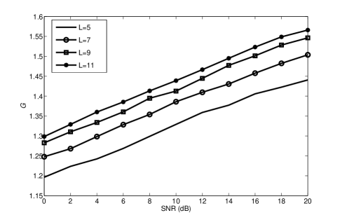
Figure 2: Capacity gain of the proposed protocol over classic protocol II.

where ${\rm E}\left[\bullet\right]$ denotes the expectation and we assume $\left\{{h_{a,b}}\right\}$ is a set of identically, independent distributed (i.i.d), complex, zero mean Gaussian random variables with unit variances. $G$ is plotted as a function of $SNR$ in Fig. 2 for different values of $L$. It is clear that the capacity gain increases as the value of SNR increases. Larger values of $L$ lead to reduced multiplexing loss and offer higher capacity gains.

IV Diversity multiplexing tradeoff

When the instantaneous CSI is not known to the transmitter, outages will occur. In this scenario diversity-multiplexing tradeoff is a powerful tool to measure the balance between the rates and error probability. In this section we study further the diversity multiplexing tradeoff [33] for such a protocol. For simplicity our analysis is based on the assumption that the signals are correctly decoded at the relays. We note that this analysis can provide insights on the best possible performance this scheme can offer. We summarize our results in the following.

Theorem 2

Define the diversity gain $d$ and multiplexing gain $r$ as those in [33]. Conditioned on the relays correctly decoding the signals (i.e, (14) and (16)), the diversity multiplexing tradeoff for the successive relaying scheme in a slow fading scenario, where the channel coefficients remain the same for $L+1$ time slots, can be expressed as:

$$d(r)=2\left(1-\frac{L+1}{L}r\right)^{+}.$$ (33)

Proof:

See Appendix. ∎

As predicted in the previous section, we can see from this theorem that a maximal diversity gain of 2 can be obtained, while the multiplexing gain can be recovered to nearly 1 for large $L$. This will offer a significant advantage in terms of spectral efficiency, which will be shown through simulations in the next section. Table I compares the maximal diversity and multiplexing gains between the successive relaying protocol and the classic protocols in a slow fading scenario. Note that for a faster fading scenario where the channel coefficient changes in every transmission time slot, the same theorem still holds if the signal transmitted in each time slot is independently encoded. Furthermore, we note that it is possible to obtain the same diversity-multiplexing tradeoff performance if proper adaptive protocols similar to those in [2] are used to consider the conditions of the source to relay links [36].

V Simulation results

In this section we make further comparison of the above protocols for different network geometries in terms of achievable rates. We compare only Classic Protocol II with the proposed protocol. As mentioned previously, to achieve better capacity performance in practice, the classic protocols should be combined with adaptive protocols so that relaying is applied only if the source to relay channels are good. There are a number of ways to enable adaptive protocols. Three examples are to base adaptation on one of the following conditions: (a) $\min\left({\left|{h_{S,R1}}\right|,\left|{h_{S,R2}}\right|}\right)\geq\left|{h_{S,D}}\right|$, i.e. the source to relay link is better than the direct link; (b) condition (16) holds; or (c) condition (31) holds. Although (b) and (c) fits better with the analysis in this paper, condition (a) is the simplest since it does not require knowledge of the relay to destination links. In the following we will only adopt (a) in the simulations. I.e, if condition (a) is not met, the system will use direct transmission. Similar results would be obtained if condition (b) or (c) were to be adopted instead.

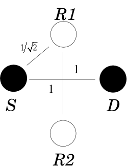
(b) Case II

(c) Case III

Figure 3: Network models for different geometries.

Our simulations are based on three network geometries: cases I, II and III, which are shown in Fig.3. We assume that each $h_{a,b}$ contains Rayleigh fading, pathloss and independent lognormal shadowing terms. These terms can be written as $h_{a,b}={v_{a,b}}\sqrt{{x_{a,b}}^{-\gamma}10^{\zeta_{k}/10}}$, where $\left\{{v_{a,b}}\right\}$ is a set of i.i.d. complex Gaussian random variables with unit variances, and $x_{a,b}$ is the distance between the nodes $a$ and $b$. The scalar $\gamma$ denotes the path loss exponent (in this paper it is always set to 4). The lognormal shadowing term $\zeta_{k}$ is a random variable drawn from a normal distribution with a mean of $0$ dB and a standard deviation $\delta=8$ (dB). We assume that the distance between the source and destination is normalized to unit distance. In case I, the distances between the source to relays and relays to destination are all normalized, so the distance between the two relays is therefore $\sqrt{3}$. In case II, the distance between relays is normalized, while the distance between the source to relays and relays to destinations is $1/\sqrt{2}$. In case III, the relays are located in the middle region between the source and destination, so that the distance between the source and relays is $1/2$ while the distance between the relays is negligible compared with the source to relays links. For the proposed protocol, these three cases represent a meaningful tradeoff between the strength of source to relay channels and the interference channel between the two relays.

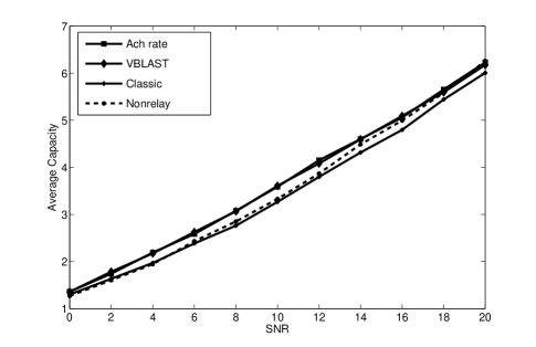
(a) Case I

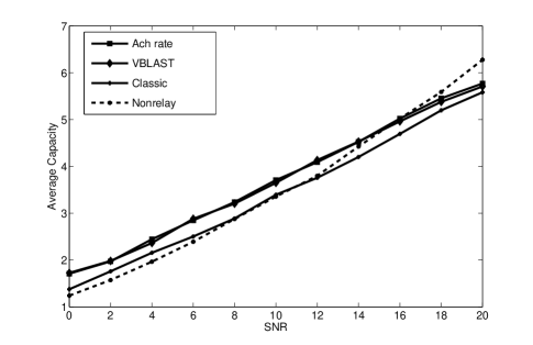
(b) Case II

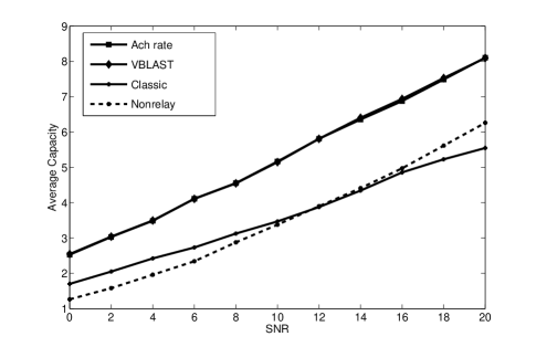
(c) Case III

Figure 4: Average capacity of the network for different network geometries in bits per transmission time slot.

We assume $L=7$ in the simulation, and the performance for the proposed protocol will certainly increase as $L$ increases. Fig.4 shows the achievable rates for the proposed protocols (ach rate), the capacity achieved by V-BLAST MMSE detection (VBLAST), the classic protocols (classic) and direct transmission (direct), all averaged over $10,000$ channel realizations. It can be clearly seen from all three figures that the V-BLAST algorithm approaches the capacity bounds for the protocol proposed in this paper.

Both Fig.4(a) and Fig. 4(b) imply that it is generally not helpful to implement relaying protocols when the source to relay link is about the same quality as the source to destination (direct) link, as the link gain due to relaying is small in this case. However, the proposed protocol still offers a performance gain over direct transmission for both the high and low SNR regions in these cases. Compared with case I and II, in case III the source to relay links are much stronger, and the relays become close to each other so that the interference is sufficiently strong to allow interference free transmission, as discussed in Sections III and IV. It can be clearly seen in Fig. 4(c) that the proposed protocol gives a significant performance advantage over direct transmission for both low and high SNR regions due to its combining gain and negligible multiplexing loss. The classic protocol still performs worse than direct transmission due to its significant multiplexing loss compared with direct transmission, although its performance gain over direct transmission for the low SNR region is improved.

VI Conclusions

In this paper we have analyzed successive relaying protocol. Our analysis shows that this protocol can maintain combining/diversity gain while recovering the multiplexing loss associated with the classic protocol. We have proposed the use of a low complexity V-BLAST detection algorithm to help implement this protocol effectively. From the simulation study based on different geometries, we can draw two main conclusions: (a) For both the proposed and classic protocols, the network capacity increases when the source-relay link becomes stronger; (b) in this scenario, while the classic protocol still loses its performance advantage for the high SNR region, the proposed protocol can give significant performance advantages for both the low and high SNR regions.

Note that one very important factor that impairs the capacity performance of the proposed protocol is interference between the two relays. Our capacity analysis does not offer the optimal capacity results for this protocol because the optimal method of suppressing the interference between the relays is not known in general. For the adaptive protocol discussed in the paper, it is also worthwhile to develop alterative forms of the protocol that explicitly account for the impact of interference between relays on the network capacity. Also it should be interesting to extend the analysis into a more than two relay scenario. These are interesting topics for future work.

[Proof of Theorem 1]

As mentioned in Section III.E, conditioned on the event that the relays correctly decode the message, the successive relaying protocol mimics a multiple access MIMO channel (5) with a capacity constraints (6) - (8). For each constraint there is a probability of not meeting it. The probability of outage is the highest among all these probabilities. Therefore there are $(2^{L}-1)$ diversity-multiplexing tradeoffs for all those conditions and the lowest curve within the range of multiplexing gain is the optimal tradeoff curve for the system [35]. To characterize the diversity-multiplexing tradeoff achieved by each constraint, we consider an $(m+1)\times m$ MIMO channel matrix ${\bf{H}}_{m}$ in the same form as in (5). Define $v_{0}$ as the exponential order [9] of $1/|h_{S,D}|^{2}$ and $v_{k}$ as the exponential order of $1/|h_{r_{k},D}|^{2}$. Furthermore, Let $\textbf{M}_{m+1}=\textbf{I}+\frac{1}{2}\Sigma_{S}\Sigma_{n}^{-1}$, where $\Sigma_{S}$ and $\Sigma_{n}$ denote the covariance matrices of the observed signal and noise components at the receiver, respectively. We assume that each source message $s_{i}$ is chosen from a Gaussian random codebook of codeword length $l$. When $m=1$, the upper bound on the ML conditional pair-wise error probability (PEP) can be calculated by

$$P_{PE\left|{v_{0},v_{1}}\right.} \leq \det\left({\textbf{I}+\frac{1}{2}\Sigma_{S_{1}}\Sigma_{n}^{-1}}\right)^{-l}$$ (34)

$$= {}\left({1+\frac{1}{2}\rho\left|{h_{S,D}}\right|^{2}+\frac{1}{2}\rho\left|{h_{r_{1},D}}\right|^{2}}\right)^{-l}$$

$$\dot{=} {}\rho^{-l(\max\{1-v_{0},1-v_{1}\})^{+}}$$

where $\dot{=}$ denotes the exponential equality [33] and $SNR$ is replaced by $\rho$ for notational simplicity. We assume each $s_{i}$ is transmitted with data rate $R$ bits in each transmission time slot. Since the successive relaying protocol uses $(L+1)$ time slots to transmit $L$ different symbols, the average transmission rate is $\overline{R}=\frac{L}{L+1}R$. On assuming that average transmission rate changes as $\overline{R}=r\log\rho$ with respect to $\rho$, then it is easy to see $R=\frac{L+1}{L}r\log\rho$. Therefore, we have a total of $\rho^{\frac{L+1}{L}rl}$ codewords. Thus, the error probability can be bounded by

$$P_{E|v_{0},v_{1}}\dot{\leq}\rho^{-l((\max\{1-v_{0},1-v_{1}\})^{+}-\frac{L+1}{L}r)}.$$ (35)

Next, we want to find the set in which the outage event always dominates the error probability performance. The analysis regarding this is similar to that in [9] and is thus omitted here. This set is given by

$$O^{+}=\left\{{(v_{0},v_{1})\in R^{2+}}\mathrel{\left|{\vphantom{(v_{0},v_{1})\in R^{2+}|(\max\{1-v_{0},1-v_{1}\})^{+}\leq\frac{L+1}{L}r}}\right.\kern-1.2pt}{(\max\{1-v_{0},1-v_{1}\})^{+}\leq\frac{L+1}{L}r}\right\}.$$ (36)

Then, for any error event which belongs to the non-outage set, we can choose $l$ to make its probability sufficiently small to ensure that the error performance is dominated by the outage probability, which can be expressed as $\rho^{-d_{o}(r)}$ for $d_{o}(r)=\mathop{\inf}\limits_{(v_{0},v_{1})\in O^{+}}(v_{0}+v_{1})$. Now using (36), $d_{o}(r)$ can be calculated as

$$d_{o}(r)=2\left(1-\frac{L+1}{L}r\right)^{+}$$ (37)

which represents the diversity-multiplexing tradeoff in the case $m=1$. When $m\geq 2$, the analysis of the determinant of $\textbf{M}_{m+1}$ can be conducted in a way similar to that in [32]; so we omit the specific calculation due to limited space. Define $D_{k}:=\det(\textbf{M}_{(k)})$, where $\textbf{M}_{(k)}$ denotes a $k\times k$ sub-matrix formed by the first $k$ rows and $k$ columns from the upper left-most corner of M. The coefficients of $D_{m+1}$ can be calculated recursively as

$$D_{m+1}\left(\frac{1}{2}\rho|h_{S,D}|^{2}\right)=\left(\frac{1}{2}\rho|h_{S,D}|^{2}\right)^{m}+\prod\limits_{j=1}^{m}{\left(1+\frac{1}{2}\rho|h_{r_{j},D}|^{2}\right)}+P\left(\frac{1}{2}\rho|h_{S,D}|^{2}\right)$$

where $P(\frac{1}{2}\rho|h_{S,D}|^{2})$ is a polynomial in $\frac{1}{2}\rho|h_{S,D}|^{2}$ and is always nonnegative. Thus, we have

$$D_{m+1}\geq\left(\frac{1}{2}\rho|h_{S,D}|^{2}\right)^{m}+\prod\limits_{k=1}^{m}{\left(1+\frac{1}{2}\rho|h_{r_{k},D}|^{2}\right)}.$$ (38)

Since we assume a slow fading environment, $v_{1}=v_{3}=\dots$ and $v_{2}=v_{4}=\dots$. On setting $v=\max\{v_{1},v_{2}\}$, it can be seen that

$$\det({\bf I}+\Sigma_{S_{m}}\Sigma_{n}^{-1})\dot{\geq}\rho^{\max\{m(1-v_{0})^{+},m(1-v)^{+}\}}.$$ (39)

If we define $\det({\bf I}+\Sigma_{S_{m}}\Sigma_{n}^{-1})\dot{=}\rho^{f(v_{0},v_{1},v_{2})}$ and

$$\rho^{\max\{m(1-v_{0})^{+},m(1-v)^{+}\}}\dot{=}\rho^{g(v_{0},v_{1},v_{2})},$$ (40)

then we have

$$f(v_{0},v_{1},v_{2})\dot{\geq}g(v_{0},v_{1},v_{2}),~{}~{}~{}~{}~{}\forall(v_{0},v_{1},v_{2})\in R^{3+}.$$ (41)

Similarly to the analysis for $m=1$, $O_{f}^{+}$ should be defined as

$$\ O_{f}^{+}=\left\{{(v_{0},v_{1},v_{2})\in R^{3+}}\mathrel{\left|{\vphantom{(v_{0},v_{1},v_{2})\in R^{3+}f(v_{0},v_{1},v_{2})\leq\frac{L+1}{L}mr}}\right.\kern-1.2pt}{f(v_{0},v_{1},v_{2})\leq\frac{L+1}{L}mr}\right\}$$ (42)

where $m$ denotes that $m$ symbols are transmitted and the equivalent data rate $R=\frac{L+1}{L}mr\log\rho$. We define

$$O_{g}^{+}=\left\{{(v_{0},v_{1},v_{2})\in R^{3+}}\mathrel{\left|{\vphantom{(v_{0},v_{1},v_{2})\in R^{3+}g(v_{0},v_{1},v_{2})\leq\frac{L+1}{L}mr}}\right.\kern-1.2pt}{f(v_{0},v_{1},v_{2})\leq\frac{L+1}{L}mr}\right\}.$$ (43)

Because of (41), it can be seen that $O_{f}^{+}\subseteq O_{g}^{+}$. Therefore

$$\mathop{\inf}\limits_{(v_{0},v_{1},v_{2})\in O_{f}^{+}}(v_{0}+v_{1}+v_{2})\geq\mathop{\inf}\limits_{(v_{0},v_{1},v_{2})\in O_{g}^{+}}(v_{0}+v_{1}+v_{2}),$$

which means that the diversity gain calculated from $O_{f}^{+}$ is always larger than that calculated from $O_{g}^{+}$.

From (40) and (43), it is not difficult to show that

$$\mathop{\inf}\limits_{(v_{0},v_{1},v_{2})\in O_{g}^{+}}(v_{0}+v_{1}+v_{2})\geq 2\left(1-\frac{L+1}{L}r\right)^{+}.$$ (44)

Comparing (37) and (44), we can see that the diversity gain achieved by a multiple access MIMO channel with channel matrix $\textbf{H}_{m}$ $(m>1)$is always larger than that for $\textbf{H}_{1}$.

Now we consider the product of the determinants of $n$ matrices $\prod\limits_{i=1}^{n}{\det({\bf I}+\frac{1}{2}\Sigma_{S_{m_{i}}}\Sigma_{n}^{-1})}$, which is related to all other rate constraints from (6) - (8). Using (39), it is easy to obtain

$$\prod\limits_{i=1}^{n}{\det\left({\bf I}+\frac{1}{2}\Sigma_{S_{m_{i}}}\Sigma_{n}^{-1}\right)}\dot{\geq}\rho^{\max\{(\sum_{i=1}^{n}m_{i})(1-v_{0})^{+},(\sum_{i=1}^{n}m_{i})(1-v)^{+}\}}$$

Define $\rho^{f_{n}(v_{0},v_{1},v_{2})}\dot{=}\prod\limits_{i=1}^{n}{\det({\bf I}+\frac{1}{2}\Sigma_{S_{m_{i}}}\Sigma_{n}^{-1})}$ and $\rho^{g_{n}(v_{0},v_{1},v_{2})}\dot{=}\rho^{\max\{(\sum_{i=1}^{n}m_{i})(1-v_{0})^{+},(\sum_{i=1}^{n}m_{i})(1-v)^{+}\}}$. It can be seen that

$$f_{n}(v_{0},v_{1},v_{2})\dot{\geq}g_{n}(v_{0},v_{1},v_{2}),~{}~{}~{}~{}~{}\forall(v_{0},v_{1},v_{2})\in R^{3+}.$$ (45)

Similarly, applying $O_{g_{n}}^{+}=\{(v_{0},v_{1},v_{2})\in R^{3+}|g(v_{0},v_{1},v_{2})\leq\frac{L+1}{L}(\sum_{i=1}^{n}m_{i})r\}$, we have that

$$\mathop{\inf}\limits_{v_{0},v_{1},v_{2}\in O_{f_{n}}^{+}}(v_{0}+v_{1}+v_{2})\geq 2\left(1-\frac{L+1}{L}r\right)^{+}.$$

The determinant of the matrix $({\bf I}+\frac{1}{2}\Sigma_{S}\Sigma_{n}^{-1})$ can always be decomposed into the product of the determinants of several submatrices $({\bf I}+\frac{1}{2}\Sigma_{S_{mi}}\Sigma_{n}^{-1})$. Therefore the error exponent is always larger than or equal to $2(1-\frac{L+1}{L}r)^{+}$ and the proof is complete.

(a) Time slot 1.

(b) Time slot 2.

(c) Time slot 3.

Figure 1: Transmission schedule for the proposed protocol.

Schemes/Maximum Gain	Multiplexing	Diversity
Direct transmission	1	1
Classic I	1/3	3
Classic II	1/2	3
Proposed scheme	$L/(L+1)$	2

TABLE I: Comparison of the different transmission schemes for the two relay case

(a) Case I

References

- [1] A. Sendonaris, E. Erkip and B. Aazhang, “User cooperative diversity-Part I and II,” IEEE Trans. Commun, vol. 51, no. 11, pp. 1927-1938, Nov. 2003.
- [2] J. N. Laneman, D. N. C. Tse and G. W. Wornell, “Cooperative diversity in wireless networks: Efficient protocols and outage behavior,” IEEE Trans. Inf. Theory, vol. 50, no. 12, pp. 3062-3080, December 2004.
- [3] J. N. Laneman and G. W. Wornell, “Distributed space-time-coded protocols for exploiting cooperative diversity in wireless networks,” IEEE Trans. Inf. Theory, vol. 49, pp. 2415-2425, Oct. 2003.
- [4] R. U. Nabar, et al. , “Fading relay channels: Performance limits and space-time signal design,” IEEE J. Sel. Areas Comm., vol. 22, no. 6, pp. 1099-1109, Aug. 2004.
- [5] B. Rankov and A. Wittneben, “Spectral efficient signaling for half-duplex relay channels,” in Proc. Asilomar Conf. Signals, syst., comput., Pacific Grove, CA, Nov.,2005.
- [6] B. Rankov and A. Wittneben, “Spectral efficient protocols for non-regenerative half-duplex relaying,” in Proc. 43th Annual Allerton Conf. Comm., Contr. and Comp., Monticello, IL, Oct. 2005.
- [7] E Zimmermann, P. Herhold and G. Fettweis, “On the performance of cooperative diversity protocols in practical wireless systems,” Proc. 2003 IEEE Vehicular Tech. Conf. - Fall, Orlando, Florida, Oct. 2003.
- [8] P.A. Anghel, G. Leus and M. Kavehl, “Multi-user space-time coding in cooperative networks,” Proc. 2003 IEEE Int’l. Conf. Acoustic, Speech & Sig. Processing, Hong Kong, China, Apr. 2003.
- [9] K. Azarian, H. El Gamal, and P. Schniter, “On the achievable diversity-multiplexing tradeoff in half-duplex cooperative channels,” IEEE Trans. Inf. Theory, vol 51, no. 12 pp. 4152-4172, Dec. 2005.
- [10] Y. Zhao, R. Adve and T. J. Lim, “Improving amplify-and-forward relay networks: Optimal power allocation versus selection,” submitted to IEEE. Trans. Wireless. Commun., Feb. 2006.
- [11] Y. Zhao, R. Adve and T. J. Lim, “Outage probability at arbitrary SNR with cooperative diversity,” IEEE Commun. Lett., vol 9, no. 8, pp. 700-702, Aug. 2005.
- [12] M. Janani, et al., “Coded cooperation in wireless communications: space-time transmission and iterative decoding,” IEEE. Trans. Signal Process., vol. 52, no. 2, pp. 362-371, Feb. 2004.
- [13] M. Costa, “On the Gaussian interference channel,” IEEE. Trans. Inf. Theory, vol. 31, no. 5, pp. 607-615, Sep. 1985.
- [14] B. Suard, et al., “Uplink channel capacity of space-division-multiple-access schemes,” IEEE Trans. Inf. Theory, vol. 44, no. 4, pp. 1468-1476, Jul. 1998.
- [15] T. Cover and J. A. Thomas, Elements of Information Theory, Wiley: New York, 1991.
- [16] R. Pabst, et al., “Relay-based deployment concepts for wireless and mobile broadband radio,” IEEE Commun. Mag., vol. 42, no. 9, pp. 80-89, Sep. 2004.
- [17] Y. Fan and J. S. Thompson, “MIMO configurations for relay channels: Theory and practice,” submitted to IEEE Trans. Wireless. Commun., to appear, 2007.
- [18] A. Bletsas, A. Lippnian, D. P. Reed, “A simple distributed method for relay selection in cooperative diversity wireless networks, based on reciprocity and channel measurements,” Proc. 2005 IEEE Vehicular Tech. Conf. - Spring, Stockholm, May - Jun. 2005.
- [19] J. Cho and Z. J. Haas, “On the throughput enhancement of the downstream channel in cellular radio networks through multihop relaying,” IEEE. J. Sel. Areas Commun., vol. 22, no. 7, pp. 1206-1219, Sep. 2004.
- [20] A. Bletsas, et al., “A simple cooperative diversity method based on network path selection,” IEEE J. Sel. Areas Commun. vol. 24, no. 3, pp. 659-672, Mar. 2006.
- [21] G. J. Foschini, et al., ”Analysis and performance of some basic space-time architectures,” IEEE J. Sel. Areas Commun., Vol. 21, No. 3, pp. 303-320, Apr. 2003.
- [22] G. J. Foschini, et al., “Simplified processing for high spectral efficiency wireless communications employing multi-element arrays,” IEEE J. Sel. Areas Commun., vol. 17, no.11, pp. 1841-1852, 1999.
- [23] S. Verdu and S. Shamai,“Spectral efficiency of CDMA with random spreading,” IEEE Trans. Inf. Theory, vol. 45, no. 2, pp. 622-640, Mar. 1999.
- [24] P. A. Anghel and M. Kaveh, “On the performance of distributed space-time coding systems with one or two non-regenerative relays,” IEEE Trans. Wireless Comm., vol. 5, no. 3, pp. 682-692, Mar. 2006.
- [25] M. Janani, et al., “Coded cooperation in wireless communications: space-time transmission and iterative decoding,” IEEE. Trans. Signal Process., vol. 52, no. 2, pp. 362?C371, Feb. 2004.
- [26] A. Stefanov and E. Erkip, “Cooperative coding for wireless networks,” IEEE Trans. Commun., vol. 52, no. 9, pp. 1470-1476, Sept. 2005.
- [27] T. E. Hunter and A. Nosratinia, “Diversity through coded cooperation,” IEEE Trans. Wireless Comm., vol. 5, no. 2, pp. 283-289, Feb. 2006.
- [28] P. Razaghi and W. Yu, “Bilayer low-density parity-check codes for decode-and-forward in relay channels,” submitted to IEEE Trans. Inf. Theory, September, 2006.
- [29] A. Wittneben and B. Rankov, “Impact of cooperative relays on the capacity of rank-deficient MIMO channels,” Proc. 12th IST Summit on Mobile and Wireless Commun., Aveiro, Portugal, pp. 421-425, June 2003.
- [30] T. Oechtering and A. Sezgin, “A new cooperative transmission scheme using the space-time delay code,” Proc. ITG Workshop Smart Antenna, pp. 41-48, Zurich, Mar. 2004.
- [31] S. Yang, J.-C. Belfiore, “Towards the optimal amplify and forward cooperative diversity scheme,” presented at the 35th IEEE Comm. Theory. Workshop, Dorado, Puerto Rico, May 2006.
- [32] S. Yang, J.-C. Belfiore, “On slotted amplify-and-forward cooperative diversity schemes,” Proc. 2006 IEEE Int’l. Sym. Inf. Theory, Seattle, USA, July 2006.
- [33] L. Zheng and D. Tse, “Diversity and multiplexing: A fundamental tradeoff in multiple antenna channels,” IEEE Trans. Inf. Theory, vol. 49, no. 5, pp. 1073-1096, May 2003.
- [34] R. A. Horn and C. R. Johnson, Matrix Analysis, Cambridge University Press, Cambridge, UK, 1985.
- [35] D. Tse, P. Viswanath and L. Zheng, “Diversity multiplexing tradeoff in multiple access channels,” IEEE Trans. Inf. Theory, vol. 50, no. 9, pp. 1859 - 1874, Sep 2004.
- [36] C. Wang, Y. Fan, J. S. Thompson and H. V. Poor, “Adaptive protocols for relay channels,” in preparation.