Scalar resonances: scattering and production amplitudes

Abstract

Scattering and production amplitudes involving scalar resonances are known, according to Watson’s theorem, to share the same phase $\delta(s)$. We show that, at low energies, the production amplitude is fully determined by the combination of $\delta(s)$ with another phase $\omega(s)$, which describes intermediate two-meson propagation and is theoretically unambiguous. Our main result is a simple and almost model independent expression, which generalizes the usual $K$-matrix unitarization procedure and is suited to be used in analyses of production data involving scalar resonances.

In reactions such as $D^{+}\rightarrow\pi^{+}\pi^{-}\pi^{+}$ or $D^{+}\rightarrow\pi^{+}K^{-}\pi^{+}$, Dalitz plots of experimental data display a wealth of resonating states (see for instance E791 ; Meadows ), indicating that contributions from final state interactions (FSIs) to observed quantities are important. In order to disentangle basic interactions from this kind of empirical information, a reliable theoretical description of the final three-meson system is required. As the full treatment of this problem is rather involved, one usually resorts to an approximation, which consists in assuming that one of the final mesons acts as a spectator. The limitations of this approximation are not well established and the issue is being debated Meadows ; Caprini . In this quasi two-body approach, theoretical work becomes much simpler, since one deals with two-body FSIs directly related with elastic scattering. This idea underlies Watson’s theorem Watson , which was produced more than fifty years ago and states that the same phase $\delta(s)$ occurs in both scattering and production amplitudes. Important as it is, the theorem does not determine how scattering information is to be used in the interpretation of production data and one finds a multitude of mutually contradictory prescriptions in the literature. In particular, there are parametrized production expressions based on either $(\sin\delta)$ BediagaMiranda ; Babar or $(\cos\delta)$ Achasov ; Pennington ; CLEO ; Furman . In other cases, expressions used in data analyses bear no connection with the scattering phase. For instance, the pioneering study of the $\sigma(500)$ scalar resonance in the decay $D^{+}\to\pi^{+}\pi^{-}\pi^{+}$ E791 was based on a trial amplitude of the form

$$\mathcal{A}=a_{nr}\mathcal{A}_{nr}+\sum_{n}a_{n}\mathcal{A}_{n}^{res},$$ (1)

where $nr$ stands for a non-resonant background, the $\mathcal{A}_{n}^{res}$ represent the contributions of various resonances and the complex weights $a_{i}$ are determined from fitting to the data. The main ingredient of the $\mathcal{A}_{n}^{res}$ amplitudes is a relativistic Breit-Wigner function, aimed at describing resonance propagation and decay. This expression makes no use of the $\pi\pi$ scattering amplitude. An obvious problem with this loose adoption of trial functions to interpret empirical data is that information about the position of the resonance pole in the complex energy plane becomes contaminated by unreliable assumptions.

We tackle the scattering-production problem in the case of a scalar resonance. In order to simplify the notation, we refrain from writing angular momentum or isospin labels explicitly in amplitudes and phases. We assume that the scalar resonance $R$ is coupled to a pair of pseudoscalar mesons $P_{a}P_{b}$ which, in practice, represents systems such as $\pi\pi$, $\pi K$, $K\bar{K}$, in the presence of $\sigma(500)$, $\kappa(800)$ and $f_{0}(980)$ resonances. The meson masses are $\mu_{a}$ and $\mu_{b}$. As we are mostly interested in relatively low-energy processes involving pions and kaons, in this work we follow both the conceptual and mathematical descriptions of resonances proposed in Ref. Pich .

The amplitude $T$ describing the elastic process $P_{a}P_{b}\rightarrow P_{a}P_{b}$ must respect unitarity, and below the first inelastic threshold, it can always be written as

$$T(s)={\cal{S}}\,\frac{16\pi}{\rho(s)}\,\sin\delta(s)\,e^{i\delta(s)},$$ (2)

where ${\cal{S}}$ is a statistical factor such that $P_{a}=P_{b}\rightarrow{\cal{S}}=2$, $P_{a}\neq P_{b}\rightarrow{\cal{S}}=1$, and $\rho(s)=\sqrt{[1-(\mu_{a}+\mu_{b})^{2}/s][1-(\mu_{a}-\mu_{b})^{2}/s]}$. Unitarity is implemented automatically in this parametrization, by means of the real function $\delta(s)$, which encompasses the full dynamical content of the interaction.

In decays of heavy mesons, such as $D$ or $B$, a part of the width may be due to the direct production of a resonance at the weak vertex. When this happens, FSIs become important and the interpolation between the decay vertex and the observed $|{P_{a}P_{b}}\rangle$ state is described by the subset of diagrams shown in Fig. 1, involving both the bare resonance propagator and the unitarized elastic scattering amplitude Achasov ; CLEO . This subset of Feynman diagrams is represented by the function $\Pi(s)$ and, for the sake of conciseness, referred to as production subamplitude.

At low energies, $\Pi(s)$ is designed to replace the Breit-Wigner function associated with the scalar resonance in Eq. (1) and has the advantage of exhibiting a clear relation to the scattering amplitude. We demonstrate, in the sequence, that it can be expressed in terms of the elastic phase $\delta(s)$ as

$$\mathrm{\bf{form\;\;1:}}\;\;\;\Pi(s)=g\;\frac{\cos\delta(s)}{m_{R}^{2}-s}\,\left[1+\frac{\tan\delta(s)}{\tan\omega(s)}\right]\,e^{i\delta(s)},$$ (3)

where $g$ is the resonance-mesons coupling constant, $m_{R}$ is the nominal resonance mass, such that $\delta(s=m_{R}^{2})=\pi/2$, and $\omega(s)$ is a meson loop phase given by

$$\tan\omega(s)=\frac{\pi\rho(s)}{\Re[L(s)-L(m_{R}^{2})]},$$ (4)

where,

$$\Re L(s)=\rho(s)\log\left[\frac{\sqrt{s-(\mu_{a}-\mu_{b})^{2}}-\sqrt{s-(\mu_{a}+\mu_{b})^{2}}}{\sqrt{s-(\mu_{a}-\mu_{b})^{2}}+\sqrt{s-(\mu_{a}+\mu_{b})^{2}}}\right]-\frac{\mu_{b}^{2}-\mu_{a}^{2}}{s}\log\left(\frac{\mu_{b}}{\mu_{a}}\right).$$ (5)

This is our main result. Simple manipulations allow it to be recast in two alternative forms, namely

$$\mathrm{\bf{form\;\;2:}} \Pi(s)=g\;\frac{\cos\delta(s)}{{\cal{M}}^{2}(s)-s}\,e^{i\delta(s)},$$ (6)

$$\mathrm{\bf{form\;\;3:}} \Pi(s)=g\;\frac{\sin\delta(s)}{m_{R}\,\Gamma(s)}\,e^{i\delta(s)},$$ (7)

where ${\cal{M}}(s)$ is a running mass and $\Gamma(s)$ is a running width. It is important to note that these two functions are not independent, since both of them are unambiguously determined by the phase $\omega(s)$.

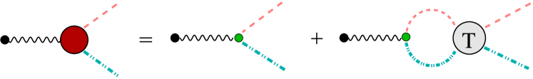
Figure 1: Resonance (wavy line) propagation and decay into mesons $P_{a}$ (dashed line) and $P_{b}$ (dot-dashed line). $T$ stands for the the unitary scattering amplitude, Eq. (2).

We now demonstrate the results given by Eqs. (3)-(7). In the spirit of the Bethe-Salpeter equation, the dynamical content of a unitarized elastic scattering amplitude can be realized as a series involving kernels and propagators. This idea is represented in Fig. 2, where the iteration of the kernel ${\cal{K}}$ by means of a two-body mesonic Green’s function yields the full amplitude $T$.

In the case of low-energy meson-meson scattering, the problem is much simplified by the fact that the two-body propagator can be described by a renormalized analytic loop function, which we denote by $\bar{\Omega}(s)$. In order to construct it, we note that the finite part of the two-meson propagator is given by a function $L(s)$ such that

$$\bullet \,\,\mbox{for}\,\,0<s<(\mu_{b}-\mu_{a})^{2}$$

$$L(s)=\rho(s)\log\left[\frac{\sqrt{(\mu_{a}+\mu_{b})^{2}-s}+\sqrt{(\mu_{a}-\mu_{b})^{2}-s}}{\sqrt{(\mu_{a}+\mu_{b})^{2}-s}-\sqrt{(\mu_{a}-\mu_{b})^{2}-s}}\right]-\frac{(\mu_{b}^{2}-\mu_{a}^{2})}{s}\log\left(\frac{\mu_{b}}{\mu_{a}}\right),$$ (8)

$$\bullet \,\,\mbox{for}\,\,(\mu_{b}-\mu_{a})^{2}<s<(\mu_{b}+\mu_{a})^{2}$$

$$L(s)=\frac{\sqrt{-\lambda(s)}}{s}\left\{\tan^{-1}\left[\frac{\mu_{a}^{2}+\mu_{b}^{2}-s}{\sqrt{-\lambda(s)}}\right]-\frac{\pi}{2}\right\}-\frac{(\mu_{b}^{2}-\mu_{a}^{2})}{s}\log\left(\frac{\mu_{b}}{\mu_{a}}\right),$$ (9)

$$\bullet \,\,\mbox{for}\,\,s>(\mu_{b}+\mu_{a})^{2}$$

$$L(s)=\rho(s)\log\left[\frac{\sqrt{s-(\mu_{a}-\mu_{b})^{2}}-\sqrt{s-(\mu_{a}+\mu_{b})^{2}}}{\sqrt{s-(\mu_{a}-\mu_{b})^{2}}+\sqrt{s-(\mu_{a}+\mu_{b})^{2}}}\right]-\frac{(\mu_{b}^{2}-\mu_{a}^{2})}{s}\log\left(\frac{\mu_{b}}{\mu_{a}}\right)+i\pi\rho(s),$$ (10)

where $\lambda(s)=(s-\mu_{a}^{2}-\mu_{b}^{2})^{2}-4\mu_{a}^{2}\mu_{b}^{2}$. The expression for $L(s)$ is simplified if $\mu_{a}=\mu_{b}$ and can be found in Robilotta . Above threshold, the function $\bar{\Omega}(s)$ is written as

$$\bar{\Omega}(s) = -\frac{1}{{\cal{S}}\,16\pi^{2}}\left\{\Re\left[L(s)-L(m_{R}^{2})\right]+i\,\Im L(s)\right\}$$ (11)

$$\equiv \bar{R}(s)+iI(s)$$

and, by construction, $\bar{R}(m_{R}^{2})=0$. The imaginary component is particularly simple and reads $I(s)=-\rho(s)/({\cal{S}}\,16\pi)$. The phase $\omega(s)$ entering Eq. (4) is defined as

$$\tan\omega(s)\equiv I(s)/\bar{R}(s)\;.$$ (12)

The representation of $T$ given in Fig.2 corresponds to a geometrical series and yields

$$T={\cal{K}}+{\cal{K}}(-\bar{\Omega}){\cal{K}}+{\cal{K}}(-\bar{\Omega}){\cal{K}}(-\bar{\Omega}){\cal{K}}+\cdots=\frac{{\cal{K}}}{1+\bar{\Omega}{\cal{K}}}.$$ (13)

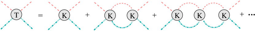
Figure 2: Geometrical series for the elastic unitary $P_{a}P_{b}$ scattering $T$-matrix. $K$ stands for the kernel, Eq. (14).

In a theory containing a resonance as an explicit degree of freedom, it is convenient to factorize its $s$-channel denominator in the kernel ${\cal{K}}$ and we write

$${\cal{K}}\equiv\frac{\gamma^{2}(s)}{m_{R}^{2}-s}\;,$$ (14)

where $\gamma(s)$ is a function satisfying the condition $\gamma(m_{R}^{2})\neq 0$. It is important to stress that Eq. (14) corresponds just to a definition, which is completely independent of dynamical assumptions. The specific form of $\gamma(s)$ for $\pi\pi$ scattering in the framework of a $SU(2)$ implementation of chiral symmetry was discussed in Ref. Robilotta , but it may be ignored in the present work. Using Eq.(14) into Eq.(13), one finds

$$T={\cal{S}}\,\frac{16\pi}{\rho(s)}\;\frac{m_{R}\,\Gamma(s)}{{\cal{M}}^{2}(s)-s-i\,m_{R}\,\Gamma(s)}\;,$$ (15)

where we have defined a running mass and a running width by

$${\cal{M}}^{2}(s)\equiv m_{R}^{2}+\gamma^{2}(s)\,\bar{R}(s)\;,$$ (16)

$$m_{R}\,\Gamma(s)\equiv\frac{\gamma^{2}(s)\,\rho(s)}{{\cal{S}}\,16\pi}$$ (17)

and, by construction, ${\cal{M}}^{2}(m_{R}^{2})=m_{R}^{2}$. Comparing this result with Eq.(2), one has

$$\tan\delta(s)=\frac{m_{R}\,\Gamma(s)}{{\cal{M}}^{2}(s)-s}\;.$$ (18)

On the other hand, the elimination of $\gamma^{2}(s)$ from Eqs. (16) and (17) makes the constraint between the running functions evident and allows one to write

$$\frac{1}{{\cal{M}}^{2}(s)-s}=\frac{1}{m_{R}^{2}-s}\left(1+\frac{\tan\delta(s)}{\tan\omega(s)}\right),$$ (19)

after using Eq.(12). This result plays an important role in our derivation, because it indicates that the running mass is completely determined just by the information contained in the empirical function $\delta(s)$ and the theoretically reliable phase $\omega(s)$.

The production subamplitude $\Pi(s)$ can be evaluated directly from Fig. 1 and reads

$$\Pi(s)=\frac{g}{m_{R}^{2}-s}\left[1+(-\bar{\Omega})\frac{{\cal{K}}}{1+\bar{\Omega}{\cal{K}}}\right]=\frac{g}{m_{R}^{2}-s}\left[\frac{1}{1+\bar{\Omega}{\cal{K}}}\right].$$ (20)

As stressed by Pennington Pennington , this shows that production and scattering share a “universal denominator”, namely $(1+\bar{\Omega}\,{\cal{K}})$, which imposes the Watson phase to the production subamplitude and transmits the physical poles from one amplitude to the other. Using Eqs. (13) and (14), one finds Eq. (7)

$$\Pi(s)=\frac{g}{\gamma^{2}(s)}\left[\frac{{\cal{K}}}{1+\bar{\Omega}\,{\cal{K}}}\right]=\frac{g\,T}{\gamma^{2}(s)}=\frac{g}{m_{R}\Gamma(s)}\sin\delta(s)e^{i\delta(s)},$$ (21)

which is form 3. Using Eq. (18) it can be transformed into form 2, Eq. (6). Finally, Eq. (19) yields form 1, Eq (3). This concludes our demonstration.

Another interesting relationship that can be derived from Eqs. (3) and (21) is

$${\cal{K}}=\mathcal{S}\frac{16\pi}{\rho(s)}\frac{\tan\delta}{\left(1+\tan\delta/\tan\omega\right)},$$ (22)

showing that the kernel is determined just by $\delta$ and $\omega$.

Results (3)-(7) extend previous ones available in the literature. Our unitarization, based on the $\bar{\Omega}$ two-body Green’s function, generalises the usual $K$-matrix approach Achasov ; Black . In the latter, the particles propagating inside the loop are taken to be on-shell, which amounts to ignoring the real part of $\bar{\Omega}(s)$: making $\bar{R}\to 0$ in Eq. (11), one has $\cot\omega\to 0$ and ${\cal{M}}^{2}\to m_{R}^{2}$. The deviation of form 1 from the $K$-matrix result is quantified by the factor $(1+\tan\delta/\tan\omega)$.

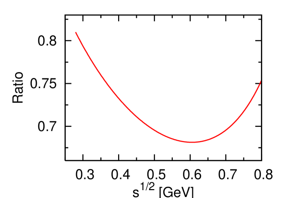
Figure 3: Ratio of the result from the $K$-matrix approximation to our Eq. (3), given by $(1+\tan\delta_{0}^{0}/\tan\omega)^{-1}$, for the $\pi\pi$ system.

In order to produce a feeling for the numerical importance of this discrepancy, we concentrate on the $\pi\pi$ system and adopt the parametrization for the scalar-isoscalar phase shift $\delta_{0}^{0}(s)$ quoted by Colangelo, Gasser and Leutwyler (CGL) CGL . We compute $\Pi(s)/g$ using Eq. (3) and identifying $m_{R}$ with their $\sqrt{s_{0}}=0.846$ GeV, which corresponds to $\delta_{0}^{0}(s_{0})=\pi/2$. We show in Fig. 3 the ratio of the result obtained in a $K$-matrix approach to ours and note that the former is typically $20-30\%$ smaller in the range $2\mu_{\pi}<\sqrt{s}<0.8$ GeV. In Fig. 4 we show results for the real and imaginary parts of $\Pi(s)/g$, as well as its modulus. The profile of $|\Pi(s)/g|$ has a broad peak-like structure close to the $\sigma(500)$ pole position quoted in CGL namely, $\sqrt{s_{\sigma}}\approx 0.475-i0.290$ GeV. This agrees with both empirical peaks in production experiments E791 ; BES ; CLEO and theoretical works dealing with pionic FSIs based on Chiral Perturbation Theory MeissnerOller ; MeissnerGardner .

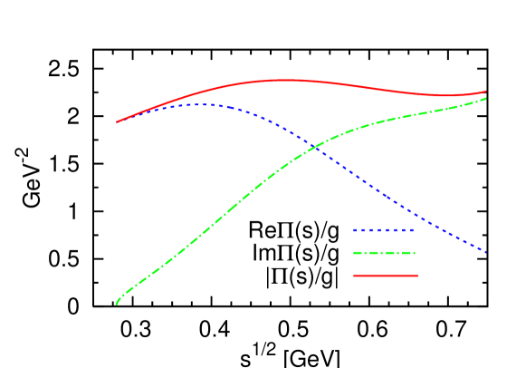
Figure 4: Result for $\Pi(s)/g$ obtained by means of Eq. (3) using $\delta_{0}^{0}(s)$ from CGL .

In summary, we have presented a prescription that allows the production subamplitude of a low-energy scalar resonance to be determined from the elastic scattering phase, supplemented by another one, describing a two-meson Green’s function. This prescription has a number of nice features, namely:

1. It has very little model dependence. As far as dynamics is concerned, the only assumption made is that the kernel entering the Bethe-Salpeter structure shown in Fig. 2 can be considered as point-like at low-energies. This assumption, which is standard in the study of mesonic systems by means of effective theories, allows one to use the rather well known bubble-like two-meson propagator.

2. It contains the $K$-matrix approach as a particular case. In that approach, corrections from the meson loops to the resonance mass are neglecteded. However, as shown in Fig. 3 for the $\pi\pi$ system, the loss of accuracy induced by this simplification is of the order of 30% in the region of physical interest.

3. It gives rise to a bump which is also visible in experiments for the $\pi\pi$ case.

4. It indicates, by means of alternative forms 2 and 3, that expressions involving both ($\sin\delta$) and ($\cos\delta$) are acceptable, provided the coherent running mass and width are used. In case other forms for these functions are adopted, consistency is lost and results may go astray.

5. It shows that precise measurements of both scattering and production amplitudes can produce direct information about the meson-meson interaction kernel. The effects of the unitarization procedure, encoded in the $\bar{\Omega}$ function, can be separated from the low-energy dynamics of the scattering process, which is represented by the function $\gamma^{2}(s)$ in Eq. (14). Using Eq. (22) one learns that this function can be determined from $\delta$ and $\omega$. This is important because $\gamma^{2}(s)$ shapes the denominator of Eq. (15) and plays a crucial role in the extraction of resonance parameters by means of pole extrapolation. Last, but not least, Eq. (22) yields directly ${\cal{K}}$ in terms of $\delta$ and $\omega$.

6. It complements Watson’s theorem, by showing that scattering and production amplitudes share not only a phase, but also neat information about the meson-meson interaction kernel.

7. It can be tested experimentally by simply replacing a Breit-Wigner function with $\Pi(s)$ in Eq. (1).

A more detailed analysis of production data involving $\pi\pi$ and $\pi K$ resonances using the formalism developed here is in progress.

- (1) E. M. Aitala et al. (E791), Phys. Rev. Lett. 86 770 (2001).
- (2) E. M. Aitala et al. (E791), Phys. Rev. D 73, 032004 (2006) [Erratum-ibid. D 74, 059901 (2006)].
- (3) I. Caprini, Phys. Lett. B 638, 468 (2006).
- (4) K. M. Watson, Phys. Rev. 88, 1163 (1952).
- (5) I. Bediaga and J. M. de Miranda, Phys. Lett. B 633, 167 (2006).
- (6) B. Aubert et al. [BABAR Collaboration], Phys. Rev. D 76, 011102 (2007).
- (7) N. N. Achasov and G. N. Shestakov, Phys. Rev. D 49, 5779 (1994).
- (8) M. R. Pennington, arXiv:hep-ph/9710456.
- (9) G. Bonvicini et al. [CLEO Collaboration], Phys. Rev. D 76, 012001 (2007).
- (10) A. Furman, R. Kaminski, L. Lesniak and B. Loiseau, Phys. Lett. B 622 207 (2005).
- (11) G. Ecker, J. Gasser, A. Pich and E. de Rafael, Nucl. Phys. B 321, 311 (1989).
- (12) L. O. Arantes and M. R. Robilotta, Phys. Rev. D 73 034028 (2006).
- (13) J. A. Oller and E. Oset, Nucl. Phys. A 620, 438 (1997) [Erratum-ibid. A 652, 407 (1999)]
- (14) D. Black, A. H. Fariborz, S. Moussa, S. Nasri and J. Schechter, Phys. Rev. D 64, 014031 (2001).
- (15) G. Colangelo, J. Gasser and H. Leutwyler, Nucl. Phys. B 603, 125 (2001).
- (16) I. Caprini, G. Colangelo and H. Leutwyler, Phys. Rev. Lett. 96, 132001 (2006).
- (17) M. Ablikim et al. (BES), Phys. Lett. B 598, 149 (2004).
- (18) Ulf-G. Meißner and J. A. Oller, Nucl. Phys. A 679, 671 (2001).
- (19) S. Gardner and Ulf-G. Meißner, Phys. Rev. D 65 094004 (2002).