Chemical chronology of the Southern Coalsack

Abstract

We demonstrate how the observed H₂O ice column densities toward three dense globules in the Southern Coalsack could be used to constrain the ages of these sources. We derive ages of $\sim 10^{5}$ yr, in agreement with dynamical studies of these objects. We have modelled the chemical evolution of the globules, and show how the molecular abundances are controlled by both the gas density and the initial chemical conditions as the globules formed. Based on our derived ages, we predict the column densities of several species of interest. These predictions should be straightforward to test by performing molecular line observations.

1 Introduction

Chemical reactions alter the composition of dense interstellar gas and theoretical models of this evolution offer the prospect of determining the relative ages of dense cores and molecular clouds (e.g., Stahler 1984; Leung, Herbst & Huebner 1984). The accuracy of these derived ages will increase with that of the initial conditions of the model calculations, i.e. knowledge of the chemical state of the gas at some arbitrary time in the past. In regions of active star formation the prompt ($t$$\buildrel<\over{\sim}\$1yr) removal of icy grain mantles of known composition, either by thermal evaporation or sputtering in shocks, almost simultaneously alters the chemical composition of protostellar cores and leads to a prolonged phase ($\sim 10^{5}$ years) of ‘hot core’ chemical evolution. The destruction of abundant ‘parent’ molecules and the formation of ‘daughter’ species in principle allows the time since mantle removal to be measured from the presently observed gas phase composition (Charnley, Tielens & Millar 1992; Charnley 1997; Hatchell et al. 1998).

Despite the fact that they are probably formed from more diffuse material, of fairly simple chemical composition, estimating relative ‘chemical ages’ for molecular clouds and for dense (starless) cores within those clouds is more problematic. Models of quiescent dark clouds have largely been based on so-called ‘pseudo-time-dependent’ models (e.g., Leung et al. 1984). In this case, the physical conditions remain fixed at dense cloud values throughout the calculation whereas the initial conditions for the heavy elements are those expected from the diffuse interstellar medium. The chemical evolution in these purely gas phase models can be roughly divided between the abundances present at ‘early-times’, prior to a major fraction of the gas phase carbon being incorporated into CO ($\sim 10^{5}$ years), and ‘late-times’, approximately when the chemistry has reached a steady-state ($\sim 10^{6}-10^{7}$ years). Time-dependent models of dark clouds have shown that the carbon-chain molecules are best explained by ‘early-time’ chemistry whereas several other molecular abundances, such as $\rm N_{2}H^{+}$ and $\rm NH_{3}$, are closer to the predicted steady-state values. This has led to the idea that observed spatial compositional gradients (e.g. involving the carbon-chains and ammonia) are due to a differing chemical ages in individual clouds (e.g. Hirahara et al. 1992; Taylor, Morata & Williams 1998).

Much effort has been made by theoretical astrochemists to reconcile the apparent chemical youth of molecular clouds with other evidence which suggests that these objects are long-lived entities (e.g., Nejad, Williams & Charnley 1990). For example, in the ‘classical’ picture of molecular cloud evolution and low-mass star formation (Shu, Adams & Lizano 1987), the ambipolar diffusion time-scale of a plasma with fractional ionization $x_{\rm e}$

$${t_{\rm AD}~{}=~{}7.3\times 10^{6}\left({x_{\rm e}\over 10^{-7}}\right)\rm~{}~{}yr}$$ (1)

(McKee et al. 1993) governs the loss of magnetic support which is a prerequisite for gravitational collapse (Shu et al. 1987). In this picture, molecular clouds are inferred to have lifetimes of $\sim 10$ Myr (Mouschovias, Tassis & Kunz 2006). However, recent studies suggest that molecular cloud formation, dissipation and star formation, are all rapid dynamical processes (Elmegreen 2000; Hartmann, Ballasteros-Paredes & Bergin 2001; Mac Low & Klessen 2004). In this revised picture, clouds form through the dissipation of supersonic turbulence and the important dynamical time-scale is the gravitational free-fall time at number density $n_{\rm H}$

$${t_{\rm ff}~{}=~{}{{4.35\times 10^{7}}{n_{\rm H}^{-1/2}}}\rm~{}~{}~{}yr}$$ (2)

Although the debate over the mode of star formation is not yet settled (e.g., Mouschovias et al. 2006; Ballesteros-Paredes & Hartmann 2006), if dense clouds and stars form within a few free-fall times, with the cloud life-time being $\sim$ 1–3 Myr (Hartmann et al. 2001), determining the chemical ages of molecular clouds may, after all, only require consideration of the abundances during the ‘early time’ phase.

To test and refine the idea that chemical models could be used to measure the (relative) ages of molecular clouds requires two additional criteria. First, we would like to model the chemical evolution in a molecular cloud for which there is independent evidence that it formed recently. The Southern Coalsack is a well-studied region which fulfills this criterion. The Coalsack is a group of molecular globules (or clumps) where the low average gas densities and the lack of discernible star formation activity (Nyman, Bronfman & Thaddeus 1989; Kato et al. 1999), the presence of a diffuse inter-clump medium, as evidenced by CH⁺ observations (Centurión, Càssola & Vladilo 1995), and the apparent dynamical youth of the major globule (Lada et al. 2004), all suggest that it is a region where simplistic chemical models may actually be applicable. Second, we would like to use another time-scale to constrain the chemical evolution. The time-scale over which icy grain mantles are laid down in molecular clouds provides a natural constraint that is independent of the precise chemical state of the gas (Charnley, Whittet & Williams 1990). This time-scale, $t_{\rm ice}$, is determined by the rate at which oxygen atoms collide with and stick to dust grains, and depends on the gas density, the atomic oxygen abundance, and the total effective grain surface area (see $\S$3).

Ice mantles have been detected towards several globules in the Southern Coalsack by Smith et al. (2002) and this allows us to estimate the mantle formation time-scale for each. In this paper, we use the mantle formation time-scale as the basic clock by which to measure the chemical chronology of dense globules in the Southern Coalsack, and thereby predict their relative chemical compositions.

2 The Southern Coalsack

The Southern Coalsack is a conspicuous dark molecular cloud complex in the southern sky. Unlike similar regions in the northern Milky Way, such as Taurus, Ophiuchius and Perseus, a striking feature of the Southern Coalsack is the, apparently complete, absence of star formation (Nyman et al. 1989; Kato et al. 1999; Bourke, Hyland & Robinson 1995; Racca, Gómez & Kenyon 2002). Optical and millimetre-wave observations of molecules towards the background field star HD 110432, which sample a line-of-sight through the inter-clump medium, show that the Southern Coalsack is pervaded by translucent ($A_{V}\approx 1-3$ mag.), diffuse ($n_{\rm H}\sim 10^{2}\rm cm^{-3}$) material (Codina et al. 1984; van Dishoeck & Black 1989; Gredel, van Dishoeck & Black 1994; Centurión et al. 1995; Rachford et al. 2001). The low CO abundance (Codina et al. 1984), and the presence of only simple molecules, are consistent with the chemistry expected in translucent clouds.

Tapia (1973) identified three dark globules (hereafter Globules 1,2 & 3) which showed higher than average extinction. Apart from isotopomers of CO, the Southern Coalsack has thus far only been mapped in OH, H₂CO, and H I (Brooks, Sinclair & Manefield 1976; McClure-Griffiths et al. 2001). Nyman et al. (1989) mapped the Southern Coalsack in CO lines and showed that Tapia’s globules were also peaks in CO emission. Observations of ¹³CO and C¹⁸O have identified several other distinct cores (Vilas-Boas, Myers & Fuller 1994; Kato et al. 1999). These studies indicate that dense condensations in the Coalsack have densities in the range $n_{\rm H}\sim 10^{3}-10^{4}~{}\rm cm^{-3}$ with gas and dust temperatures of around 10 K (Jones, Hyland & Bailey 1984). An infrared extinction study of Globule 2 (Lada et al. 2004) indicates that it is in a state of dynamical equilibrium, and suggest that it formed only recently. Thus, the Southern Coalsack is a region where dense cloud cores have recently condensed out of a more diffuse, low-extinction, interclump medium.

Smith et al. (2002) performed 3$\rm\mu m$ spectroscopy towards eight field stars, located behind the Southern Coalsack, to search for H₂O ice absorption towards several of the dense globules. Six of these sources lay behind or near Globule 2 and one behind each of the other two. Smith et al. detected water ice in each of Tapia’s globules with an additional four tentative detections in Globule 2. The largest ice column densities were found toward stars with the largest visual extinctions, as found in many other interstellar clouds (e.g., Whittett et al. 1988). In general, the fact that the water features are only apparent above a certain level of $A_{V}$ is not direct proof that the ice must be present in the densest regions, although it is suggestive that this is the case. In the Coalsack, however, the fact that Smith et al.’s field stars lay behind the globules, and we know from the CO line maps that these are regions of higher density, leads us to conclude that the observed H₂O ice is frozen out in the cold, dense globules, and not in the inter-clump medium. In what follows, we use data from Smith et al. for their sources designated SS1-2, SS2-2 and SS3-1 to derive a mantle formation time-scale in each of Tapia’s Globules 1, 2 & 3.

3 Ice formation time-scales

We now show how observations of the ice column density can be used to estimate the ice mantle formation time-scales. Accretion and hydrogenation of oxygen atoms will lead to a spherical (silicate) grain core of radius $a$ being covered by a water ice mantle, and the mean particle radius growing as

$${r(a,t)~{}=~{}a~{}+~{}d(a,t)}$$ (3)

where $d(a,t)$ is the instantaneous mean mantle thickness. A spherical grain of instantaneous radius $r(a,t)$ increases in size by accretion of mass through oxygen atoms sticking to the surface at a rate (Wickramasinghe 1967)

$${dr\over dt}~{}=~{}{S\over\rho_{\rm ice}}\left({kTm_{\rm O}\over 2\pi}\right)^{1/2}n_{\rm O}(t)$$ (4)

where $T$ is the gas temperature, $S$ is the sticking efficiency, $m_{\rm O}$ is the mass of an oxygen atom, $\rho_{\rm ice}$ is the bulk density of water ice, and $n_{\rm O}(t)$ is the number density of O atoms in the gas. For simplicity, we have ignored the increase in mass due to the accretion of two hydrogen atoms per oxygen. Because both the molecular accretion rate and the number of molecules required to build up one monolayer of coverage are proportional to the surface area of the grain, the radial growth of grains is independent of grain size. Hence, at any particular time all grains will be covered by the same thickness of ice.

An ice mantle will contain on average $W(a,t)$ water molecules

$${W(a,t)~{}=~{}{4\pi\rho_{\rm ice}\over 54m_{\rm H}}[r^{3}(a,t)~{}-~{}a^{3}]}$$ (5)

where $m_{\rm H}$ is the hydrogen nucleon mass. A pathlength $L$ through a molecular cloud with uniform dust and gas number densities, $n_{\rm gr}(a)$ and $n_{\rm H}$, has an ice column density of

$${N_{\rm ice}(t)~{}=~{}\int_{0}^{L}\int_{a_{-}}^{a_{+}}W(a,t){n_{\rm gr}(a)}~{}da~{}dl}$$ (6)

If the hydrogen column density, $N_{\rm H}$ ($=n_{\rm H}L$), is related to the visual extinction through

$${N_{\rm H}~{}=~{}1.6\times 10^{21}A_{V}\rm~{}~{}cm^{-2}}$$ (7)

(Bohlin, Savage & Drake 1978) then the time to accumulate this much ice, the mantle formation time-scale, $t_{\rm ice}$, satisfies

$${\int_{a_{-}}^{a_{+}}[r^{3}(a,\mbox{$t_{\rm ice}$})~{}-~{}a^{3}]a^{-3.5}~{}da~{}=~{}5.8\times 10^{-20}{N_{\rm ice}(\mbox{$t_{\rm ice}$})\over\rho_{\rm ice}A_{V}}}$$ (8)

Here we have assumed that the dust obeys an MRN size distribution (Mathis, Rumpl & Nordsieck 1977) such that

$${{n_{\rm gr}(a)}~{}=~{}Aa^{-3.5}n_{\rm H}}$$ (9)

in a range bounded by ${a_{-}}=0.005~{}\mu\rm m$ and ${a_{+}}=0.25~{}\mu\rm m$, and where $A=7.76\times 10^{-26}\rm cm^{2.5}/H$ for silicate dust (Draine & Lee 1984). The ice mantle thickness at this time, $d_{\rm m}=d(\mbox{$t_{\rm ice}$})$, is just $r(a,\mbox{$t_{\rm ice}$})-a$, and so we can evaulate the integral in (8) to obtain a cubic equation in $d_{\rm m}$. As $N_{\rm ice}$/$A_{V}$ is determined observationally, the cubic can be solved to obtain $d_{\rm m}$ for any source.

We must now calculate the time, $t_{\rm ice}$, required to accrete this thickness of ice. Accretion on to grains removes oxygen atoms from the gas at a rate

$${dn_{\rm O}\over dt}~{}=~{}-\frac{\Lambda_{\rm gr}(t)}{4}n_{\rm H}S\left({8kT}\over\pi m_{\rm O}\right)^{1/2}n_{\rm O}(t)$$ (10)

where the total available grain surface area per nucleon at time $t$, $\Lambda_{\rm gr}(t)$, is

$$\Lambda_{\rm gr}(t)~{}=~{}\left\langle 4\pi r^{2}(a,t)n_{\rm gr}(a)/n_{\rm H}\right\rangle$$ (11)

$$~{}~{}~{}=~{} \int_{a_{-}}^{a_{+}}4\pi r^{2}(a,t)n_{\rm gr}(a)/n_{\rm H}~{}da$$

$$~{}~{}~{}=~{} 9.75\times 10^{-25}\int_{a_{-}}^{a_{+}}r^{2}(a,t)a^{-3.5}~{}da$$

The factor of 4 in eqn. (10) is due to the fact that $\Lambda_{\rm gr}$ represents the total grain surface area ($4\pi r^{2}$), whereas the cross-section for accretion onto each grain is equal to $\pi r^{2}$.

Subject to some approximations, an analytical solution for $t_{\rm ice}$ can be obtained. Firstly, accretion on to grains is the dominant loss route for O atoms in dark clouds, so we neglect the effects of other chemical processes on $n_{\rm O}(t)$. We also assume that the underlying power-law for $n_{\rm gr}(a)$ is not modified by coagulation. For time-scales sufficiently short that $\Lambda_{\rm gr}(t)$ is approximately unchanged (i.e. only thin mantles have formed), the total surface area of the bare grains integrated over the MRN size distribution, $\Lambda_{\rm gr}(0)$, is equal to $2.37\times 10^{-21}$ cm²/H. For constant $\Lambda_{\rm gr}(0)$, the solution of eqn. (10) is

$$n_{\rm O}(t)=n_{\rm O}(0)e^{-t/t_{\rm acc}}$$ (12)

where $n_{\rm O}(0)$ is the initial gas-phase oxygen atom abundance and $t_{\rm acc}$ is their accretion time-scale

$$t_{\rm acc}=\frac{1}{\Lambda_{\rm gr}(0)n_{\rm H}S}\left(\frac{2\pi m_{\rm O}}{kT}\right)^{1/2}$$ (13)

Integration of eqn. (4) then yields

$$d(t)=d_{\rm max}\left[1-e^{-t/t_{\rm acc}}\right]$$ (14)

where $d_{\rm max}=(18m_{\rm H}n_{\rm O}(0)/\Lambda_{\rm gr}(0)n_{\rm H}\rho_{\rm ice})$ is the maximum thickness of ice that can be attained when all the oxygen has frozen out. With $d_{\rm m}$ set from the observational data through equation (8), the mantle formation time is found from

$$\mbox{$t_{\rm ice}$}=t_{\rm acc}\,\ln\left[1-\frac{d_{\rm m}}{d_{\rm max}}\right]^{-1}$$ (15)

In order to calculate $t_{\rm ice}$ in the Coalsack, we adopt a sticking coefficient of unity, and assume a gas and dust temperature of 10 K (Jones et al. 1984). Experimental measurements of amorphous water ice deposited at low temperatures indicate densities in the range 0.6–1 g cm^-3, depending on the details of the ice deposition (e.g. Jenniskens & Blake 1994; Stevenson et al. 1999). Therefore, we adopt $\rho_{\rm ice}=0.75$ g cm^-3. Values of $N_{\rm ice}$, $A_{V}$, and $n_{\rm H}$ for each of the three globules are taken from the observations of Kato et al. (1999) and Smith et al. (2002). The only remaining parameter required to calculate $t_{\rm ice}$ is the initial oxygen atom abundance in the gas, which depends on the elemental abundances in the Coalsack, and on the original chemical conditions in each globule (i.e. how much oxygen was locked up in CO and other molecules). For the chemical models described in the following section, O atom abundances of $n_{\rm O}(0)/n_{\rm H}=1.6\times 10^{-4}$ and $2.9\times 10^{-4}$ are assumed, depending on whether the chemistry in each globule was initially appropriate for translucent (T) or diffuse (D) material.

Table 1 lists the physical conditions observed in each globule, and the corresponding values of $d_{\rm m}$ and $t_{\rm ice}$ derived for each object. In all cases the derived mantle thicknesses are significantly less than the maximum possible value, $d_{\rm max}$, showing that only a small fraction of the total oxygen is frozen out as water, and that each globule must be much significantly younger than the accretion time-scale. The $t_{\rm ice}$ values derived are consistent with these globules having formed recently (cf. $\sim 2\times 10^{5}$ years; Lada et al. 2004). The principal uncertainties in our derived values of $t_{\rm ice}$ come from uncertainties in the values of $\Lambda_{\rm gr}(0)$ and the initial gas-phase oxygen atom abundance. For example, if we truncate the grain size distribution at $a_{-}=100$ Å instead of 50 Å, this reduces the effective grain surface area by a factor of almost two-thirds, and thus increases the derived values of $t_{\rm ice}$ by 50 per cent. Similarly, because the initial values for $n_{\rm O}$ differ by a factor of two between models D and T, the derived ages differ by a similar factor. Hence, determining the absolute age of each core requires knowledge of the initial chemical conditions and the grain size distribution. However, it is likely that each globule coalesced from material with similar properties, and so the relative ages will be much more accurate.

Table 1: Globule properties and ice mantle formation time-scales in the Coalsack

Globule	$N_{\rm ice}^{\dagger}$	$A_{\rm V}^{\dagger}$	$n_{\rm H}^{\ddagger}$	x(CO)‡	$d_{\rm m}$	$t_{\rm ice}$(D)	$t_{\rm ice}$(T)
	$(10^{17}~{}\rm cm^{-2})$	(mag.)	$(10^{3}~{}\rm cm^{-3})$	$(10^{-5})$	(Å)	($10^{5}~{}\rm yr$)	($10^{5}~{}\rm yr$)
1	9.1	11.2	4.0	7.5	85	2.0	3.7
2	5.7	13.3	8.2	13.7	45	0.5	1.0
3	2.0	9.9	5.4	8.6	21	0.4	0.7

^† Smith et al. (2002). ^‡ Kato et al. (1999); for globule 3 we have used values quoted for their core 4. $t_{\rm ice}$(D) and $t_{\rm ice}$(T) are the ice formation time-scales corresponding to different values of the initial O atom abundance (see text).

4 Chemical model

We now want to use the derived $t_{\rm ice}$ values to find chemical discriminants of the different ages. The values of $t_{\rm ice}$ measure the time since the ice mantles began to be laid down, and it is well known that mantle formation does not occur until the visual extinction reaches a critical threshold of $A_{\rm V}\sim 3$ mag. (e.g. Whittet et al. 1988). In the Coalsack, Smith et al. (2002) derive an extinction threshold in the range 2.6–7.6 mag. Therefore, the appropriate initial conditions for the chemical model at $t=0$ are determined by the chemical state of the cloud when $A_{\rm V}\approx 3$–8 mag., which are in turn determined by the physical evolution of the cloud from the diffuse phase to a dense core. In the limit that core formation occured rapidly, the initial abundances will be identical to those in the diffuse ISM, i.e. principally atomic oxygen and nitrogen with carbon and sulphur in ionic form. On the other hand, if the cloud evolved slowly, so that it spent a long time in the ‘translucent’ phase ($1\lower 3.01385pt\hbox{$\buildrel<\over{\sim}\ $}A_{\rm V}\lower 3.01385pt\hbox{$\buildrel<\over{\sim}\ $}3$ mag.), then the cloud material will have been mainly molecular (CO and N₂, with only O atomic) when $A_{\rm V}$ reached the critical value and ices began to form. Therefore, we have considered two models corresponding to initally diffuse and translucent chemical abundances: the abundances at $t=0$ for both models are listed in table 2.

The gas-phase elemental abundances are taken from Savage & Sembach (1996), except for sulphur which is assumed to be significantly depleted relative to the diffuse ISM (Ruffle et al. 1999). In our ‘standard’ model runs we also assume complete depletion of heavy elements, although the effects of non-zero metal abundances are discussed below in $\S$5.1. The chemical reaction network is described in Rodgers & Charnley (2001), and has been updated to incorporate several recently measured dissociative recombination channels (e.g. Geppert et al. 2006). All neutral species except H₂ and He freeze out onto grain mantles with a sticking coefficient of unity. We adopt a temperature of 10 K and a cosmic ray ionization rate of $3\times 10^{-17}$ s^-1. Values for $n_{\rm H}$ and $A_{\rm V}$ are set equal to those derived for each of the three globules (table 1).

Table 2: Initial abundances relative to H₂

Species	Abundance
	Model D	Model T
C+	2.8(-4)	2(-8)
C	0	2(-5)
CO	0	2.6(-4)
O	5.8(-4)	3.2(-4)
N	1.6(-4)	0
N2	0	8(-5)
S+	1(-7)	1(-7)
He	0.2	0.2

Model D corresponds to the abundances expected if the globules condense rapidly from diffuse cloud material. In model T the initial conditions represent those in low-density translucent ($A_{\rm V}\approx 2$) gas. $a(-b)$ represents $a\times 10^{-b}$.

5 Results

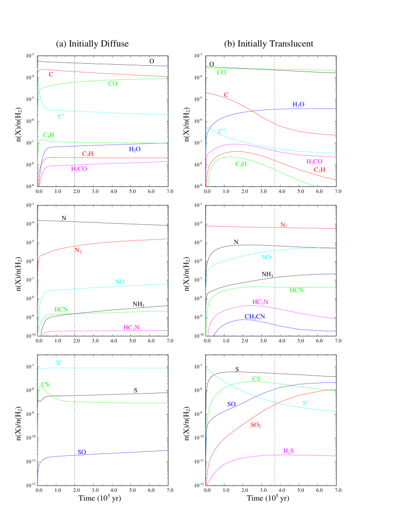
Figure 1: Chemical evolution in Coalsack Globule 1. (a) The left panels show the model results for initially diffuse cloud abundances, and (b) the right hand panels show the evolution from initially transclucent cloud conditions. The gray vertical dashed lines mark the ice mantle formation time-scale, $t_{\rm ice}$. The time-scale is longer in (b) because the initial abundance of atomic oxygen is smaller.

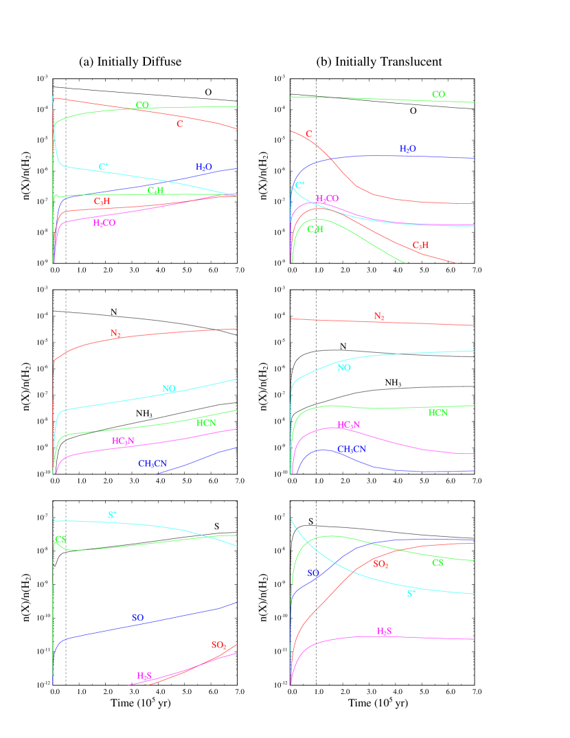
Figure 2: As figure 1, but for Globule 2.

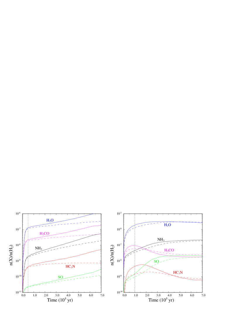
Figure 3: Effects of metals on the chemical evolution in Coalsack Globule 2. As in figures 1 and 2, the left and right panels show the results for models D and T respectively, and the gray vertical dashed lines mark the ice mantle formation time-scale, $t_{\rm ice}$. Solid lines show the results for models with zero metals, and dashed lines show the results with a silicon abundance of 10^-7.

Figure 1 shows the chemical evolution in Globule 1 for both the initially diffuse and initially translucent model runs. Also indicated on the graphs are the mantle formation timescales, $t_{\rm ice}$, derived from the H₂O ice observations. The values of $t_{\rm ice}$ are different for each model since $t_{\rm ice}$ depends on the initial abundance of atomic O. Figure 2 shows the evolution in the denser Globule 2. Globule 3 has a density intermediate to Globules 1 and 2, and the chemical evolution in this source is similar to that in Globule 1.

Table 3: Calculated molecular column densities in each of the three globules.

Molecule	Globule 1		Globule 2		Globule 3
	D	T	D	T	D	T
$t_{\rm ice}$($10^{5}$ yr)	2.0	3.7	0.5	1.0	0.4	0.7
C	4.6(17)	4.1(15)	7.0(17)	6.1(14)	1.3(18)	1.0(15)
C+	1.0(15)	1.9(14)	1.9(14)	9.2(13)	4.0(15)	1.4(14)
CO	1.3(18)	7.1(17)	1.6(18)	1.5(18)	8.3(17)	1.6(18)
CH4	7.6(15)	6.8(14)	5.3(16)	7.0(14)	6.1(14)	7.8(14)
H2CO	4.0(15)	4.5(14)	1.4(16)	1.8(14)	6.1(14)	2.0(14)
H2O	7.4(15)	1.1(16)	3.5(16)	1.9(16)	2.7(15)	2.1(16)
OH	6.6(14)	5.4(15)	5.3(14)	4.0(15)	2.1(14)	3.2(15)
O2	4.6(14)	6.2(16)	6.2(14)	1.7(17)	1.5(14)	1.1(17)
NH3	7.8(14)	4.1(15)	9.0(14)	3.0(15)	6.8(13)	1.5(15)
NO	1.6(15)	4.5(16)	1.0(15)	3.3(16)	3.1(14)	2.1(16)
HCN	6.4(14)	1.6(15)	4.6(15)	4.7(14)	1.0(14)	2.6(14)
HNC	2.9(14)	7.8(14)	1.2(15)	2.7(14)	3.4(13)	1.6(14)
CN	3.6(14)	5.8(14)	2.7(14)	1.2(14)	8.9(13)	1.2(14)
CS	3.8(14)	8.8(13)	4.8(14)	7.4(13)	2.4(14)	1.3(14)
SO	6.7(11)	9.9(13)	2.4(11)	2.5(14)	3.3(11)	1.5(14)
SO2	2.2(10)	6.0(13)	3.7(10)	1.8(14)	5.3(9)	5.6(13)
H2S	1.0(11)	4.5(11)	1.8(11)	6.0(11)	1.1(10)	3.0(11)
H2CS	3.7(13)	9.6(11)	7.0(13)	2.4(12)	6.4(12)	7.0(12)
C2H	5.7(14)	2.4(13)	3.8(14)	5.5(12)	1.1(14)	7.9(12)
C3H	3.9(15)	4.6(13)	7.6(15)	1.6(13)	1.1(15)	9.2(13)
C3N	4.9(15)	4.6(12)	2.5(16)	2.3(12)	4.7(15)	1.8(13)
C4H	4.1(15)	1.5(13)	8.7(15)	4.7(12)	2.4(15)	3.4(13)
C3H2	2.1(14)	2.9(13)	1.2(14)	7.7(12)	5.4(13)	2.1(13)
HC3N	2.5(14)	2.5(13)	3.4(15)	9.0(12)	2.6(13)	2.2(13)
HCO+	4.0(13)	9.8(13)	7.2(13)	1.4(14)	3.5(12)	1.2(14)
O	9.7(17)	3.9(17)	2.3(18)	9.0(17)	2.8(18)	1.3(18)
CH	2.4(14)	6.6(12)	2.7(14)	2.6(12)	2.8(14)	3.0(12)
CH2	2.9(13)	6.7(11)	5.3(13)	2.9(11)	5.7(13)	3.1(11)
C2H2	1.5(14)	5.7(13)	1.7(14)	5.2(13)	3.3(13)	1.1(14)
N2	4.8(17)	6.4(17)	4.2(17)	8.1(17)	1.3(17)	6.0(17)
NH	2.1(14)	1.5(15)	2.7(13)	2.8(14)	9.7(12)	1.2(14)
CH3CN	6.2(13)	1.3(13)	1.4(15)	1.6(12)	1.7(12)	1.5(12)
CH3OH	9.6(9)	4.6(10)	1.7(11)	:.0(10)	1.1(8)	1.5(11)
CH3OCH3	6.3(6)	4.2(6)	3.6(8)	6.0(6)	1.2(4)	8.3(6)
OCS	1.3(12)	4.1(11)	2.4(12)	1.7(12)	1.8(11)	1.9(12)
N2H+	9.7(12)	5.4(13)	7.0(12)	3.0(13)	3.3(11)	1.8(13)

a(b) represents $a\times 10^{b}~{}\rm cm^{-2}$.
Column densities are calculated by multiplying the abundance calculated by our chemical model at time $t_{\rm ice}$ by the H₂ column densities determined from the visual extinction measurements of Smith et al. (2002).
D and T refer to models with the initial conditions appropriate for diffuse or translucent material respectively (see table 2).

Comparing figures 1 and 2 it is apparent that although the chemical evolution of both globules is similar in many respects, the difference in density results in a slightly different chemistry in each source. If the globules formed rapidly from diffuse cloud material, it takes a long time for the conversion of the initially atomic material into predominantly molecular form, but in the denser Globule 2 the CO/C ratio becomes $>1$ after $3\times 10^{5}$ yr, whereas in the lower density Globule 1 the transition takes almost 1 Myr. The transformation of atomic nitrogen into N₂ takes even longer in each source. The large abundances of C⁰ and N⁰ act to suppress the abundances of species such as CN, NO, and SO, which in turn tend to reduce the abundances of many other species below their ‘typical’ dark cloud values. In both globules HCN, NH₃, HC₃N, and CH₃CN remain at low abundances for $t<1$ Myr, although their abundances become somewhat larger in Globule 2 at later times. Based on our values of $t_{\rm ice}$, Globule 1 is older than Globule 2, and so the difference in abundances between the two regions will not be as pronounced as if both were the same age, but we predict that in Globule 2 the abundances of H₂CO, HCN, HC₃N, and CS, should be $\approx 2$–3 times larger than in Globule 1.

The alternative scenario, in which CO and N₂ formed prior to the cores reaching the critical extinction for water ice formation to occur, results in larger abundances of several molecules, especially sulphur-bearing species. For example, SO, SO₂, and H₂S are much more abundant in panels (b) of figures 1 and 2. Again, chemical differences between the two sources arise primarily due to their different ages, and we expect that carbon chain species such as C₃H and C₄H should be 2–3 times more abundant in the younger Globule 2, whereas NH₃, SO and SO₂ should be more abundant in Globule 1.

In terms of discriminating between the two model scenarios, there are large differences in the abundances of several species. If the globules formed directly from diffuse material, the abundances of carbon-chain molecules such as C₄H will be larger than if the gas was initially molecular. On the other hand, the reduced C⁰ abundance in the latter case leads to larger abundances of many other molecules such as H₂CO, NH₃, HCN, HNC, and especially SO and SO₂. Therefore, observations of these species in the Coalsack can in principle be used to determine which model is correct. In order to allow comparison with observations, table 3 lists the column densities for selected species in each of the three globules at the appropriate time, $t_{\rm ice}$, calculated for each model.

5.1 Effects of model parameters

We have also investigated the effects of altering various parameters of our models. As discussed above, we used the elemental abundances of Savage & Sembach (1996). However, if we consider the only direct measurement taken toward the Coalsack, Jensen, Rachford & Snow (2005) reported a low elemental O/H ratio of only $6.5\times 10^{-5}$ toward HD 110432, a factor of four less than used in our model (although the error bars on this measurement are also consistent with a ‘normal’ O/H ratio.) We therefore ran our model with the abundances of all elements depleted by a factor of four. In the case of initially translucent conditions (model T) the effects are relatively minor, but for model D we find that the reduced elemental abundances act to speed up the transition from the diffuse-cloud-type chemistry to the dark-cloud-type chemistry, resulting in enhanced abundances of species such as H₂CO, NH₃, HCN, SO, and SO₂. However, a key aspect of this change is that it also increases the values of $t_{\rm ice}$ by a factor of four, since the O atom freeze-out rate is reduced. For the observed ice thicknesses in Globule 1 this implies that that this source must have an age comparable to or greater than the accretion time-scale, which is equal to 1.2 Myr. This conflicts with other evidence that the Southern Coalsack is a relatively young region (see $\S$ 2), and so we consider it likely that the elemental abundances (or at least the oxygen abundance) in the Coalsack are close to standard interstellar values.

We also investigated the effects of a non-zero metal abundance, by running each model with an initial abundance of Si⁺ equal to $10^{-7}$. We find that the effects on the chemistry of Globule 1 are minor, but in the denser Globule 2 the effects are more important. Figure 3 compares the abundances of those species most affected by the metal abundance in models D and T for Globule 2. We see that the effects are largest in model D at late times; at the early times implied by the observed water ice column densities the presence or absence of metals has little influence on the predicted abundances. One exception is HC₃N, where the early-time abundance is depressed in model T when Si⁺ is included.

6 Discussion

Most models of interstellar dark cloud chemistry assume initial conditions appropriate for diffuse clouds, i.e. they assume that the cloud formation timescale is much less than the chemical timescale. For typical dark cloud densities of $n({\rm H}_{2})=10^{4}$ cm^-3, the exact choice of the initial conditions is not so important, as the chemistry rapidly evolves from the diffuse cloud conditions into ‘standard’ dense cloud chemistry. Our results show that, for lower density gas such as the globules in the Coalsack, the transformation time may be much longer, of order Myr. In this case, the time spent in the translucent phase is a key parameter of the model, and the dense globules retain a chemical ‘memory’ of the prior conditions. Hence, in principal, molecular observations of the dark globules can be used to constrain the dynamics of their origins.

Rachford et al. (2001) observed CO and H₂ toward the field star HD 110432, and derived a CO/H₂ column density ratio of $\approx 3\times 10^{-7}$, suggesting that the molecular fraction in the inter-clump medium is low. However, at such low H₂ column densities the overall CO/H₂ ratio may be low due to CO dissociation in the outer layers where $A_{\rm V}\lower 3.01385pt\hbox{$\buildrel<\over{\sim}\ $}1$, and is still consisitent with almost all C in CO in the central regions (e.g. van Dishoeck & Black 1989). It is difficult to use such observations to tightly constrain the C/CO ratio in the interclump medium.

Although there have been several studies of dust and extinction in the Coalsack, there is a dearth of molecular line observations of this region. As far as we know, the only molecules observed in the Coalsack are CO (Huggins et al. 1977; Codina et al. 1984; Kato et al. 1999), OH, and H₂CO (Brooks et al. 1976). The latter observed the 6 cm formaldehyde $1_{11}$–$1_{10}$ line in absorption, and derived a H₂CO/H₂ abundance of $\sim$ 10^-9, at least an order of magnitude smaller than the abundances we derive for the globules in Table 3. However, the 6 cm line absorption feature appears to arise preferentially from the lower density regions surrounding the dense core rather than from the dense core itself (Snell 1981). This would appear to be confirmed by the fact that Brooks et al. report the emission from the H₂CO is extended over a size of 12 arcminutes (similar to that of the OH emission), and also by the fact that our chemical model predicts a H₂CO abundance of $\sim 10^{-9}$ in low-density, translucent material. A second effect to consider is that extinction maps reveal the densest regions of the globules are likely of order 1–3 arcminutes in size (Bok 1977; Jones et al. 1980; Lada et al. 2004), smaller than the 4 arcminute beamsize of Brooks et al. Hence, H₂CO features arising from the centers of the globules will suffer from beam dilution. We conclude that the 6 cm observations of Brooks et al. most likely trace the interclump medium.

Figure 4: Integrated pencil-beam H₂ column density (i.e. $A_{\rm v}$; solid line) and water ice column densites (dashed lines) as a function of impact parameter for a Bonnor-Ebert sphere with central density $n_{\rm H}=10^{4}$ cm^-3, appropriate for Globule 2 in the Coalsack. Ice column densities are shown at times of 2, 4, 6, 8, & 10 $\times$ $10^{5}$ yr.

We have only considered the case of a single sightline through a constant density medium since that is the nature of the observational constraints currently available to us (Smith et al. 2002). In reality, such prestellar globules have spatial density gradients, and the observed ice column density depends on the particular line-of-sight path integral through the cloud. Recent studies of the infrared extinction of field stars which lay behind these globules have allowed detailed maps to be made of the visual extinction through several globules (Alves, Lada & Lada 2001; Kandori et al. 2005). For isolated globules, the dust density profile is usually well matched by a Bonnor-Ebert sphere (Alves et al. 2001; Racca et al. 2002) and many appear to be on the critical limit of gravitational instability against runaway collapse (Kandori et al. 2005). The ice formation time-scale derived for any sightline will always lag that of the dynamical time-scale over which the mass distribution was assembled. Hence, if 3 micron observations towards fields stars behind such globules can be made to allow their radial ice profile to be constructed, this could eventually be employed as a good measure of the dynamical time. The analysis presented in this paper allows us to calculate the water ice column density as a function of both time and offset, $\xi$, from the core center in Coalsack Globule 2, where $n_{\rm H}(r,\xi)$ is from a Bonnor-Ebert sphere (Racca et al. 2002). As an example, Figure (4) shows that the ice profile has a distinctive shape at each time, and so fitting the observed $N_{\rm ice}(\xi)$ distribution with such models will allow a global derivation of $t_{\rm ice}$ for each source.

7 Conclusions

Oxygen atom accretion and reaction to form H₂O ice is a ‘one-way’ process (at least until a protostar has formed), is essentially unaffected by gas-phase chemistry, and begins only when the dense core forms. Hence, ice column densities can be employed as an independent measure of physical age. A combination of ice absorption and molecular emission observations can thus lead to quantitative measures of globule age, and allow correlations between physical and chemical evolution to be explored.

We have determined the ‘ice mantle age’, $t_{\rm ice}$, of three dense globules in the Southern Coalsack, based on the time needed to deposit the H₂O ice abundances observed by Smith et al. (2002) in these sources. In conjunction with a simple chemical model, we have used these values of $t_{\rm ice}$ to predict the abundances of numerous gas-phase molecules toward each of these sources. These predictions can be easily tested by future molecular line observations of the Coalsack. Our main findings can be summarized as follows:

• In each globule only a small fraction of the total available gas-phase oxygen is frozen out as water, indicating that each must be significantly younger than the accretion time-scale.

• We derive values for $t_{\rm ice}$ of a few times $10^{5}$ yr. for Globule 1 and $\la 10^{5}$ yr. for Globules 2 and 3. These ages are consistent with the dynamical age for Globule 2 derived by Lada et al. (2004).

• The principal uncertainty in determining exact values for $t_{\rm ice}$ arises from our lack of knowledge of the gas-phase O atom abundance in each source and the grain size distribution. However, assuming each globule formed from chemically similar gas, the relative ages of the globules are easily constrained.

• The chemical evolution is very sensitive to the initial conditions when the visual extinction becomes large enough for water ice to accrete. In particular, whether carbon and nitrogen are atomic or locked up in CO and N₂ has a profound influence on the chemistry: if ${\rm C/CO>1}$ at $t=0$, the abundances of many species are less than if the material is initially in molecular form.

• As the globules age, the abundances of some species change, and should be different in each of the three globules. Observations of several species in each of the three globules can be used to test the validity of our model.

• The relative abundances of sulphur-bearing species, particularly SO and H₂S, appear to be useful diagnostics of the differences between the various models.

• Combining water ice observations with gas-phase molecular line observations toward pre-stellar cores provides a method of dating these objects. Such measurements can potentially discriminate between ‘fast’ and ‘slow’ scenarios for molecular cloud formation.

References

- [1]
- [2] Alves, J.F., Lada, C.J., & Lada, E.A. 2001, Nature, 409, 159
- [3] Ballasteros-Paredes, J., Hartmann, L., Rev. Mex. Astron. y Astrofis., in press
- [Bohlin et al.(1978)] Bohlin, R.C., Savage, B.D., Drake, J.F., 1978, ApJ, 224, 132
- [4] Bok, B.J., 1977, PASP, 89, 597
- [5] Bourke, T.L., Hyland, A.R., Robinson, G. 1995, MNRAS, 276, 1052
- [6] Brooks J.W., Sinclair M.W., Manefield G.A., 1976, MNRAS, 175, 117
- [7] Centurión, M., Càssola, C., Vladilo, G. 1995, A&A, 302, 243
- [8] Charnley, S.B. 1997, ApJ, 481, 396
- [9] Charnley, S.B., Tielens, A.G.G.M. and Millar, T.J. 1992, ApJL, 399, L71
- [10] Charnley, S.B., Whittet, D.C.B. and Williams, D.A. 1990, MNRAS, 245, 161
- [Codina et al.(1984)] Codina, S. J., de Freitas Pacheco, J. A., Lopes, D. F., Gilra, D. 1984, A&AS, 57, 239
- [Draine & Lee(1984)] Draine, B. T., Lee, H. M., 1984, ApJ, 285, 89
- [11] Elmegreen B.G., 2000, ApJ, 530, 277
- [12] Geppert W.D. et al., 2006, in Astrochemistry Throughout the Universe: Recent Successes and Current Challenges, eds. D.C. Lis, G.A. Blake & E. Herbst, Cambridge University Press, p. 117
- [13] Gredel, R., van Dishoeck, E.F., Black, J.H. 1994, A&A, 285, 300
- [14] Hartmann L., Ballesteros-Paredes J, and Bergin E. A. 2001, ApJ, 562, 852
- [15] Hatchell, J., Thompson, M.A., Millar, T.J., MacDonald, G.H., 1998, A&A, 338, 713
- [16] Hirahara, Y. et al. 1992, ApJ, 394, 539
- [17] Huggins P.J., Gillespie A.R., Sollner T.C.L.G., Phillips T.G., 1977, A&A, 54, 955
- [Jensen et al.(2005)] Jensen, A. G., Rachford, B. L., & Snow, T. P. 2005, ApJ, 619, 891
- [18] Jenniskens P., Blake D.F., 1994, Science, 265, 753
- [Jones et al.(1980)] Jones, T.J., Hyland, A.R., Robinson, G., Smith, R., Thomas, J., 1980, ApJ, 242, 132
- [19] Jones, T.J., Hyland, A.R., Bailey, J. 1984, ApJ, 282, 675
- [20] Kandori R., et al., 2005, AJ, 130, 2166
- [Kato et al.(1999)] Kato, S., Mizuno, N., Asayama, S.-i., Mizuno, A., Ogawa, H., Fukui, Y., 1999, Pub. Astron. Soc. Japan, 51, 883
- [21] Lada, C.J., Huard, T.L., Crews, L.J., Alves, J.F. 2004, ApJ, 610, 303
- [] Leung, C.M., Herbst, E., Huebner, W.F. 1984, ApJS, 56, 231
- [] Mac Low M.-M. and Klessen R. S. 2004, Rev. Mod. Phys., 76, 125
- [Mathis et al.(1977)] Mathis, J. S., Rumpl, W., Nordsieck, K. H., 1977, ApJ, 217, 425
- [McClure-Griffiths et al.(2001)] McClure-Griffiths, N. M., Dickey, J. M., Gaensler, B. M., Green, A. J., 2001, ApJ, 562, 424
- [22] McKee, C.F., Zweibel, E.G., Goodman, A.A. and Heiles, C. 1993, in Protostars and Planets III, University of Arizona Press, Tucson, p. 327,
- [Mouschovias et al.(2006)] Mouschovias, T. C., Tassis, K., & Kunz, M. W. 2006, ApJ, 646, 1043
- [23] Nejad, L.A.M., Williams, D.A. & Charnley, S.B. 1990, MNRAS, 246, 183
- [24] Nyman, L.-Å., Bronfman, I., Thaddeus, P. 1989, A&A, 216, 185
- [25] Racca, G., Gómez, M., Kenyon, S.J. 2002, ApJ, 124, 2178
- [Rachford et al.(2001)] Rachford B.L., et al., 2001, ApJ, 555, 839
- [Rodgers & Charnley(2001)] Rodgers S.D., Charnley S.B., 2001, ApJ, 546, 324
- [Ruffle et al.(1999)] Ruffle, D. P., Hartquist, T. W., Caselli, P., & Williams, D. A. 1999, MNRAS, 306, 691
- [Savage & Sembach(1996)] Savage, B. D., & Sembach, K. R. 1996, Ann. Rev. Astron. Astrophys., 34, 279
- [Shu et al.(1987)] Shu, F. H., Adams, F. C., & Lizano, S. 1987, Ann. Rev. Astron. Astrophys., 25, 23
- [Smith et al.(2002)] Smith, R. G., Blum, R. D., Quinn, D. E., Sellgren, K., & Whittet, D. C. B. 2002, MNRAS, 330, 837
- [26] Snell, R.L., 1981, ApJ Supp., 45, 121
- [27] Stahler, S.W., 1984, ApJ, 281, 209
- [28] Stevenson K.P., Kimmel G.A., Dohnálek Z., Smith R.S., Kay B.D., 1999, Science, 283, 1505
- [29] Tapia, S. 1973, in Interstellar Dust and Related Topics, J.M. Greenberg & H.C. van de Hulst (eds.), Kluwer: Dordrecht, 43
- [30] Taylor, S.D., Morata, O., Williams, D.A. 1998, A&A, 336, 309
- [31] van Dishoeck, E.F., Black, J.H. 1989, ApJ, 340, 273
- [32] Vilas-Boas, J.W.S., Myers, P.C., Fuller, G.A. 1994, ApJ, 433, 96
- [Whittet et al.(1988)] Whittet, D. C. B., Bode, M. F., Longmore, A. J., Admason, A. J., McFadzean, A. D., Aitken, D. K., & Roche, P. F. 1988, MNRAS, 233, 321
- [33] Wickramasinghe, N.C. 1967, Interstellar Dust, Chapman and Hall, London.