BEATS OF THE MAGNETOCAPACITANCE OSCILLATIONS IN LATERAL SEMICONDUCTOR SUPERLATTICES

We present calculations on the magnetocapacitance of the two-dimensional electron gas in a lateral semiconductor superlattice under two-dimensional weak periodic potential modulation in the presence of a perpendicular magnetic field. Adopting a Gaussian broadening of magnetic-field-dependent width in the density of states, we present explicit and simple expressions for the magnetocapacitance, valid for the relevant weak magnetic fields and modulation strengths. As the modulation strength in both directions increase, beats of the magnetocapacitance oscillations are observed, in the low magnetic field range (Weiss-oscillations regime), which are absent in the one-dimensional weak modulation case.

KEYWORDS: lateral surface superlattices; density of states; magnetocapacitance.

1 Introduction

A lateral surface superlattice (LSSL) combines a system of nano-fabricated gates with a MODFET, where a periodic pattern is imposed onto 2DEG at the semiconductor heterostructure[1]. This pattern can be a one- or two-dimensional periodic potential modulation of different strength allowing for a variety of artificial periodic structures. The periodic potential is applied through an array of metal gates whose bias can be varied[2]. The modulation which is purely induced by the modulated gate potential, leads predominantly to a sinusoidal potential shape and its strength can be tuned by a nano-patterned top gate as well as by a back gate electrode[3]. Magnetotransport measurements in LSSL devices have revealed novel oscillations in the conductivity, the Weiss oscillations[4] which are superimposed on top of the well-known Shubnikov-de Haas oscillations. Weiss oscillations were first discovered in LSSL devices with holographically defined one-dimensional (1D) superlattices[5], and were explained[6, 7] in terms of a commensurability criterion between the cyclotron orbit diameter at the Fermi level $2R_{c}=2\sqrt{2\pi n_{e}}\hskip 2.0ptl^{2}$ (where $n_{e}$ is the electron density and $l=\sqrt{\hbar/eB}$ the magnetic length) and the superlattice period $\alpha$:

$$2R_{c}=(\lambda+{\phi})\alpha\hskip 12.0pt\lambda=0,1,2,...$$ (1)

where $\phi$ is a phase factor.

Besides Weiss oscillations, novel magneto-resistance oscillations with $1/B$ periodicity have been observed in short-period superlattices when one flux quantum $h/e$ passes through an integral number of lattice unit cells[8, 26]. A large fraction of these studies was performed on square[10] or rectangular lattices[11, 12], while only a few experiments on hexagonal lattices have been published[13, 14]. For the majority of the effects, the lattice type is, in principle, irrelevant. Nevertheless, Altshuler-Aronov-Spivak oscillations have been observed around zero magnetic field in hexagonal lattices, while Aronov-Bohm oscillations can be detected in larger magnetic fields[14].

The capacitance of a mesoscopic structure is of electrochemical nature. It depends in an explicit manner via the thermodynamical density of states on the electronic properties of the structure. The investigation of the magnetic-field dependence of the electrochemical capacitance plays a significant role in several experiments, especially those using capacitance spectroscopy. Capacitive studies of the density of states of a two-dimensional electron gas are possible because the thermodynamical density of states appears as a series capacitance to the geometrical capacitance[15]. The behavior of the electrochemical capacitance can be also be examined from a dynamical point of view[16]. At low frequencies, the frequency dependent capacitance can be expanded in frequency and at the linear order it is a series combination of the static capacitance and a charge relaxation resistance. This approach has been performed to the analysis of mesoscopic capacitors in Refs[17, 18].

The oscillatory characteristics caused by commensurability between the cyclotron diameter $2R_{c}$ and the modulation period $\alpha$ in a LSSL, reveal themselves in the electrochemical magnetocapacitance measurements. A pronounced modulation of both the minima and maxima of the capacitance oscillations has been observed in LSSLs with 1D weak periodic potential and explained as a consequence of the oscillatory bandwidth of the modulation-broadened Landau levels[4]. Although in recent years special attention has been paid to investigate the magnetic miniband structure as well as the magneto-transport properties in a LSSL under two-dimensional weak modulation[8, 26], magnetocapacitance calculations pertinent to this case are rather limited[19].

In this paper we present calculations on the density of states and the magnetocapacitance of the 2DEG in a LSSL under two-dimensional weak periodic potential modulation in the presence of a perpendicular magnetic field. Adopting a Gaussian broadening of magnetic-field-dependent width, we present explicit and simple expressions for the DOS, valid for the relevant weak magnetic fields and modulation strengths. We investigate the magnetocapacitance, as a function of the magnetic field, for various strengths of the periodic potential modulation. In the low-field range (Weiss-oscillations regime), a beating structure in the oscillating magnetocapacitance is observed.

The paper is organized as follows: In Section 2 we briefly present the magnetic spectrum of the 2DEG in a LSSL under two-dimensional weak periodic potential modulation. In Section 3, the DOS is calculated analytically and numerically as a function of energy and magnetic field. In section 4 we present numerical results concerning the magnetocapacitance oscillations. We conclude with a summarizing Section 5.

2 Energy spectrum under weak 2D-periodic modulation potential

To describe the electrons in the conduction band of a lateral superlattice at the AlGaAs-GaAs interface in a constant perpendicular magnetic field $\mbox{\boldmath$B$}=B\hat{z}$, we employ a model of strictly 2DEG with a 2D periodic potential modulation $V(\mbox{\boldmath$r$})$, $\hskip 3.0pt\mbox{\boldmath$r$}\equiv(x,y)$. Following the common practice, we adopt an effective mass approximation to take into account the effect of the crystalline atomic structure over the charge carriers. The system is described by the well-known single-particle Hamiltonian of Bloch electrons in a homogeneous magnetic field:

$$\mathcal{H}=\frac{1}{2m^{\star}}\big{(}\mbox{\boldmath$p$}+e\mbox{\boldmath$A$}\big{)}^{2}+V(\mbox{\boldmath$r$})$$ (2)

where we neglect the Zeeman splitting and spin-orbit interactions which are very small in GaAs systems. The effective mass $m^{\star}$ for electrons in AlGaAs-GaAs is taken $m^{\star}=0.067~{}m_{e}$, where $m_{e}$ is the free-electron mass.

We consider a two-dimensional periodic modulation with rectangular symmetry, i.e:

$$V(x,y)=V_{x}\cos{(\frac{2\pi}{a_{x}}x)}+V_{y}\cos{(\frac{2\pi}{a_{y}}y)}$$ (3)

where $V_{x}$, $V_{y}$ are the modulation strengths and $a_{x}$, $a_{y}$ the periods in the corresponding directions. We assume that the modulation is weak compared to the cyclotron energy $\hbar\omega_{c}$ so that mixing of different Landau levels can be neglected. The homogeneous magnetic field is represented by the vector potential $\mbox{\boldmath$A$}=(-By/2,-Bx/2,0)$.

Applying a direct perturbation theory[26] or a projection operator approach[20] to unmodulated system, the energy spectrum is obtained as a function of the crystal momentum $(k_{x},k_{y})$ and the number of flux quanta through a lattice-unit cell $\Phi/\Phi_{0}$, where $\Phi_{0}=h/e$ is the magnetic flux quantum.

$$E(k_{x},k_{y})=(n+\frac{1}{2}\hskip 3.0pt)\hbar\hskip 1.0pt\omega_{c}\hskip 2.0pt+V_{x}F_{n}(u_{x})\cos{(\frac{2a_{x}}{\pi}u_{x}k_{y})}+V_{y}F_{n}(u_{y})\cos{(\frac{2a_{y}}{\pi}u_{y}k_{x})}$$ (4)

where $F_{n}(u)=\exp{(-u/2)}L_{n}(u),\hskip 3.0ptu_{x}=(\pi\Phi_{0}/\Phi){a_{y}}/{a_{x}},\hskip 3.0ptu_{y}=(\pi\Phi_{0}/\Phi){a_{x}}/{a_{y}}$ and $L_{n}(u)$ are the Laguerre polynomials. The perturbation approach has been shown to be an extremely good approximation to the direct diagonalization of the Hamiltonian, for the parameter values of interest ($V_{x},V_{y}<<E_{F}$, where $E_{F}$ is the Fermi energy) and for magnetic fields $0.1~{}T<B<1~{}T$. Thus, the unperturbed Landau levels broaden into bands, with width $W_{n}(B)=2(V_{x}|F_{n}(u_{x})|+V_{y}|F_{n}(u_{y})|)$, that oscillates with magnetic field $B$.

In the low-magnetic-field range it is a good approximation to take the large n-limit of the Laguerre polynomials[21] that appear in $W_{n}(B)$. For a square lattice with $a_{x}=a_{y}=a$, the width of the bandwidth is then obtained as

$$W_{n}(B)=\frac{2(V_{x}+V_{y})}{\pi}\sqrt{\frac{a}{R_{c}}}\hskip 5.0pt\bigg{|}\cos\bigg{(}\frac{2{\pi}R_{c}}{a}-\frac{\pi}{4}\bigg{)}\bigg{|}$$ (5)

where $R_{c}=l\sqrt{2n_{F}+1}$ is the cyclotron radius with $n_{F}=E_{F}/\hbar\omega_{c}$ the Landau index at the Fermi level. From equation (5) we obtain that the bandwidth reaches zero (flat band) when $2R_{c}/a=(\lambda+1/4)$ and maximum when $2R_{c}/a=(\lambda+3/4)$ with $\lambda=0,1,2,...$ .

3 Density of States

The DOS per unit area of the 2DEG, in the absence of disorder, can be expressed as a series of $\delta$-functions:

$$D(E)=\frac{g_{s}}{2\pi l^{2}}\sum_{nk_{x}k_{y}}\delta(E-E_{nk_{x}k_{y}})\;$$ (6)

where $g_{s}=2$ is the electron-spin degeneracy.

In the case of 1D electrostatic modulation, the $\delta$-functions in Eq. (6) are broadened into bands with Van Hove singularities at the edges of each Landau band. On the other hand, if 2D modulation is imposed, the DOS does not exhibit Van Hove singularities reflecting the 2D nature of the electron motion in the Landau bands with finite mean velocities[20].

In practical two-dimensional electron systems, there is always some broadening present due to scattering centers. We assume a Gaussian broadening of zero shift and a width $\Gamma$ which, according to short-range scattering theory of Aoki and Ando[22], is proportional to $\sqrt{B}$. In this case Eq. (6) takes the form

$$\begin{array}[]{llc}D(E)&=\displaystyle{\frac{g_{s}}{2\pi l^{2}}}\sum_{nk_{x}k_{y}}\frac{1}{\sqrt{2\pi}\Gamma}\exp{\bigg{(}-(E-E_{nk_{x}k_{y}})^{2}/2\Gamma^{2}\bigg{)}}\\ &=\displaystyle{\frac{g_{s}}{2\pi^{3}l^{2}}\sum_{n}\int_{0}^{\pi}}dt_{x}\int_{0}^{\pi}dt_{y}\frac{1}{\sqrt{2\pi}\Gamma}\exp{\bigg{(}-(E-E_{nt_{x}t_{y}})^{2}/2\Gamma^{2}\bigg{)}}\end{array}$$ (9)

We expand the integrand of Eq. (9) in powers of $\epsilon_{n,t_{i}}=V_{i}F_{n}(u_{i})cos(t_{i})$, $i=x,y$, assuming weak modulation strengths. The odd powers of $\epsilon_{n,t_{i}}$ vanish after integrating over $t_{x}$ and $t_{y}$. Then, to second order in the modulation potential, the even powers can be easily integrated and finally we obtain

$$\frac{D(E)}{D_{0}}=\frac{\hbar\omega_{c}}{\sqrt{\pi}}\frac{1}{\Gamma}\sum_{n}e^{-(E-E_{n})^{2}/\Gamma^{2}}\Big{[}1+\frac{\Delta_{n}^{2}}{2}\frac{2(E-E_{n})^{2}-\Gamma^{2}}{\Gamma^{4}}\Big{]}$$ (10)

where $\Delta_{n}^{2}=|V_{x}F_{n}(u_{x})|^{2}+|V_{y}F_{n}(u_{y})|^{2}$ and $D_{0}=m^{\star}/\pi\hbar^{2}$ is the DOS of a free 2DEG at $B=0$. Near the center of the $\it{n}th$ Landau level, the expression is valid only when $|V_{i}F_{n}(u_{i})|^{2}\leq\Gamma$, $i=x,y$.

Using the Poisson’s summation formula[21], we carry out the summation over $\it{n}$ and the DOS becomes

$$\begin{array}[]{llc}\displaystyle{\frac{D(E)}{D_{0}}}=1&-\frac{\displaystyle{1}}{\displaystyle{4\pi}}\bigg{(}\displaystyle{\frac{V_{x}}{E}}\bigg{)}^{2}\kappa_{x}\exp{\big{(}-(\kappa_{x}\Gamma/2E)^{2}\big{)}}\Big{[}\sin{(2\kappa_{x})}+\cos{(2\kappa_{x})/\kappa_{x}}\Big{]}\\ &\\ &-\displaystyle{\frac{1}{4\pi}\bigg{(}\frac{V_{y}}{E}\bigg{)}^{2}\kappa_{y}\exp{\big{(}-(\kappa_{y}\Gamma/2E)^{2}\big{)}}\Big{[}\sin{(2\kappa_{y})}+\cos{(2\kappa_{y})/\kappa_{y}}\Big{]}}\\ &\\ &+2\displaystyle{\sum\raisebox{-10.76385pt}{ \mbox{\scriptsize$n$}}}\hskip 5.0pt(-1)^{n}\exp{\big{(}-(n\pi\Gamma/\hbar\omega_{c})^{2}\big{)}}\cos{(2\pi nE/\hbar\omega_{c})}\\ &\\ &\times\Big{[}1-\displaystyle{\frac{2\pi n^{2}}{\kappa_{x}}\Big{(}\frac{V_{x}}{\hbar\omega_{c}}\Big{)}^{2}\cos^{2}{(\kappa_{x}-\frac{\pi}{4})}-\frac{2\pi n^{2}}{\kappa_{y}}\Big{(}\frac{V_{y}}{\hbar\omega_{c}}\Big{)}^{2}\cos^{2}{(\kappa_{y}-\frac{\pi}{4})}\Big{]}}\end{array}$$ (18)

where

$$\kappa_{x}=\sqrt{\frac{2E}{\hbar\omega_{c}}}\hskip 4.0pt\frac{2{\pi}l}{a_{x}},\hskip 10.0pt\kappa_{y}=\sqrt{\frac{2E}{\hbar\omega_{c}}}\hskip 4.0pt\frac{2{\pi}l}{a_{y}}$$ (19)

Figure 1(a) shows the DOS as a function of energy. We have adopted

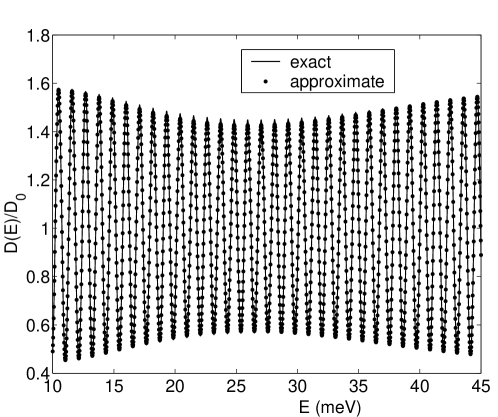
(a)

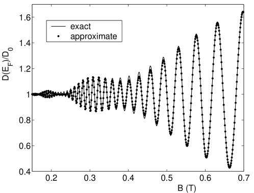
(b)

Figure 1: Calculated DOS of a 2DEG in a periodic 2D electrostatic modulation (a) as a function of energy at $B=0.64$ T and (b) as a function of magnetic field B. The solid curve corresponds to exact numerical results and the dotted to approximate from Eq.(18). The parameters used are $V_{x}=V_{y}=0.3$ meV, $a_{x}=a_{y}=365$ nm, $E_{F}=11.43$ meV, $\Gamma=0.35\sqrt{B}$ meV.

a field-dependent width $\Gamma=0.35\sqrt{B}$ meV which is consistent with most of the earlier numerical studies in the low magnetic field range[23]. The other parameters used in the numerical calculation are $V_{x}=V_{y}=0.3$ meV, $B=0.64$ T, $a_{x}=a_{y}=365$ nm. The solid curve shows the result from the analytic expression (18) and the doted one is obtained numerically from Eq. (9). As it can be seen, the agreement between the curves is good for most of the energies. In Figure 1(b) we show the DOS at the Fermi energy as a function of the magnetic field. The Fermi energy is evaluated for given electron density $n_{e}$ inserting Eq. (6) in the relation

$$n_{e}=\int_{0}^{\infty}dEf(E-E_{F})D(E)$$ (20)

where $f(x)=[1+e^{x/KT}]^{-1}$ is the Fermi-Dirac distribution function. For the parameters listed above, the correction to the Fermi energy due to weak two-dimensional modulation, is found to be of order $10^{-3}$ over the range $B<0.7$ T and hence, for $n_{e}=3.2\times 10^{11}$ $cm^{-2}$, a fixed value of $E_{F}=11.43$  meV has been adopted. Good agreement is found between the numerical and the approximate curves except at certain magnetic fields for which the amplitude of the DOS-oscillations is slightly underestimated. The DOS exhibits a peak at each Landau-band center. We observe that the weak 2D-periodic potential produces clear modulation of the envelope of the DOS-oscillations and a beating structure appears in the range $0.15~{}T<B<0.45~{}T$ (Weiss - oscillations regime). The above beating structure is not observed in the 1D weak modulation case.

4 Beats in the magnetocapacitance oscillations

The capacitance of a system consisting of a metal gate-insulator-semiconductor sandwich (e.g. gated AlGaAs/GaAs heterostructure), depends not only on the thickness of the insulator but also on the DOS at the semiconductor side and on the material’s parameters. If the two depletion layers interpenetrate each other, the gate voltage $V_{G}$, is connected to the electron density by[24]

$$V_{G}=\frac{eL}{\epsilon_{i}}n_{e}+\frac{E_{F}}{e}+K$$ (21)

where $L$ is the thickness of the AlGaAs-layer, $\epsilon_{i}$ is the dielectric constant of the layer and $K$ is a constant that takes into account fixed charges in the AlGaAs. Differentiating Eq.(21) with respect to $n_{e}$, one obtain the total inverse magneto-capacitance[25] per unit area $C(B)$ at a given temperature T:

$$\frac{1}{C(B)}-\frac{1}{C_{0}}=\frac{1}{e^{2}D_{T}(0)}\Big{[}\ \frac{D_{T}(0)}{D_{T}(B)}-1\Big{]}$$ (22)

where $C_{0}$ denotes the total capacitance at zero magnetic field, and

$$D_{T}(B)=\frac{\partial n_{s}}{\partial E_{F}}=\int_{0}^{\infty}dED(E)\frac{df(E-E_{F})}{dE_{F}}$$ (23)

Expression (22) is valid when a change in the gate voltage affect only the charge in the 2DEG and the gate, leaving intact the charge of impurities in the heterostucture. This condition is fulfilled at low temperatures in a LSSL based on AlGaAs/GaAs heterostructure. Following a dynamical approach[16], an analogue expression has been recently derived by Wang et.al.[26] for the frequency dependent electrochemical capacitance in order to study high-frequency inductive corrections in a quantum capacitor similar to the experiment of Gabelli et.al.[27]

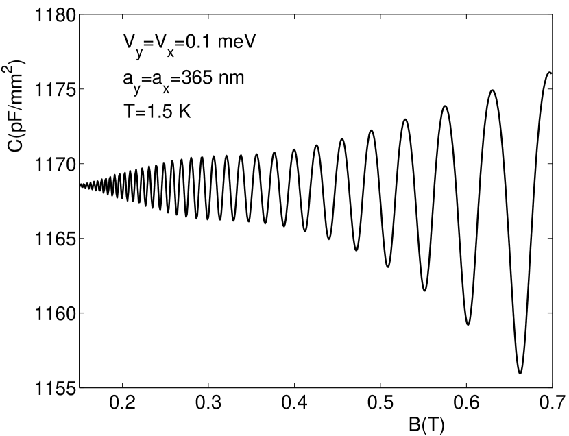
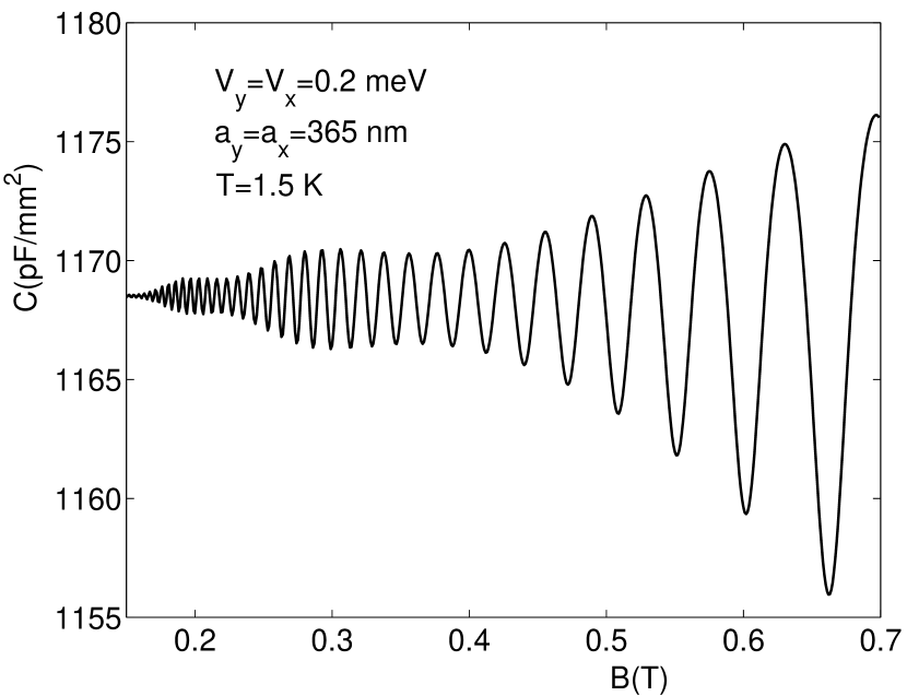
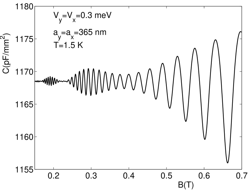
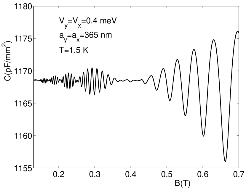
Figure 2: Calculated magnetocapacitance versus magnetic field for potential strengths $V_{x}=V_{y}=0.1,~{}0.2,~{}0.3,~{}0.4$ meV, scattering broadening $\Gamma=0.35\sqrt{B}$ meV, and periods $a_{x}=a_{y}=365$ nm.

Figure 2 shows our numerical results for the capacitance between the gate and the 2DEG as a function of magnetic field at temperature $T=1.5$ K. We consider the case of square-symmetric modulation with $a_{x}=a_{y}=365$ nm and $V_{x}=V_{y}=0.1,~{}0.2,~{}0.3,~{}0.4$ meV. The zero-filed capacitance has been taken from experiment[29] equal to $C_{0}=1168$ pF/ mm². As the modulation strength in both directions increases, modulated magnetocapacitance oscillations with nodes (a beating pattern) are observed in the low magnetic filed range $0.15~{}T<B<0.45~{}T$. The phases of the oscillations changes at these nodes and the number as well as the amplitude of beatings increases as the modulation strength increases. We should note that the potential strengths, are kept in the weak modulation regime ($V_{x}<<E_{F},V_{y}<<E_{F}$), so that Landau Level mixing is prevented. Concerning larger magnetic fields $B>0.5$ T (Shubnikov-de Hass oscillations range), the envelope of magnetocapacitance maxima increases monotonically with increasing magnetic field, while the the envelope of the magnetocapacitance minima decreases monotonically with increasing magnetic field.

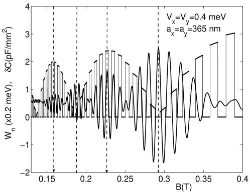
Figure 3: Modulated bandwidth $W_{n}(B)$ and beating patterns of magnetocapacitance oscillations for the square $LSSL$ with $a_{x}=a_{y}=365$ nm and $V_{x}=V_{y}=0.4$ meV.

The origin of the above beating structure is the oscillatory behavior of the bi-directionally modulated bandwidth. This behavior is clearly shown in Figure 3 where the contribution ${\delta}C(B)=C(B)-C_{0}$ is plotted together with the bandwidth oscillations in the magnetic-field range of interest. The beatings of the magnetocapacitance oscillations, at a certain magnetic field $B$, correspond to adjacent minima or maxima of the modulated bandwidth $W_{n}(B)$ and the amplitudes of the oscillations under each envelope are closely related to the value of $W_{n}(B)$. In other words, the beatings occur nearly in the middle between adjacent ‘flat-band’ conditions. Especially, for the beating structure of Figure 3, we found that the cental peaks of the beatings appear at the magnetic fields $B=0.157~{}T,~{}0.185~{}T,~{}0.227~{}T,~{}0.292~{}T$. These values coincide with the magnetic fields given by the following commensurability relation derived from Eq.(1)

$$B_{\lambda}=\frac{2\hbar\sqrt{2\pi n_{e}}}{ea(\lambda+\phi)}$$ (24)

with $\phi=\pm 1/4$ and $\lambda=2,~{}3$.

5 Concluding Remarks

We have studied the magnetocapacitance oscillations of a 2DEG in a LSSL under 2D weak periodic modulations at low temperatures ($T\sim 1$ K). Adopting a Gaussian broadening of magnetic-field-dependent width, an explicit analytic expression for the oscillatory behavior of the DOS has been obtained. An overall agreement between the exact and approximate results is found for the relevant weak magnetic fields ($B<1$ T) and modulation strengths ($V_{x}<<E_{F},V_{y}<<E_{F}$). The calculated magnetocapacitance has been shown to have a rich oscillatory structure in this regime. As the modulation strength in both directions increases, a beating pattern is observed in the low magnetic field range $0.15~{}T<B<0.45~{}T$ due to the oscillatory behavior of the bi-directionally modulated Landau-level bandwidth. It is our aim to extend our calculations for the case of a square LSSL with non-symmetric 2D modulation as well as the case of a LSSL with different periods in both directions. We are not aware of any directly relevant experimental work. We hope though that the results described above will motivate experiments in which the low-field magnetocapacitance could be measured in a weakly bi-directionally modulated 2DEG of a LSSL.

References

- [1] U. Rossler and M. Suhrke,Ad. Solid State Phys. 40 (2000) 35.
- [2] F. M. Peeters and J. D. Boeck, Handbook of Nanostructured Materials and Nanotechnology Vol. 3, H. S. Nalwa, Ed., New York: Academic Press, 2000, ch. 7.
- [3] S. Lindemann et al., Phys. Rev. B66 (2002) 165317.
- [4] D. Weiss, K. v. Klitzing, K. Ploog and G. Weimann, Phys. Rev. Lett. 62 (1989) 179; D. Weiss, C. Zhang, R. R. Gerhardts, K. v. Klitzing and G. Weimann, Phys. Rev. B39 (1989) 13020.
- [5] R. W. Winkler, J. P. Kotthaus and K. Ploog Phys. Rev. Lett. 62 (1989) 1177.
- [6] C. W. J. Beenakker , Phys. Rev. Lett.62 (1989) 2020.
- [7] R. R. Gerhardts, D. Weiss, and K. v. Klitzing, Phys. Rev. Lett. 62, (1989) 1173; R. R. Gerhardts, D. Weiss, and U. Wulf, Phys. Rev. B43 (1991) R5192.
- [8] S. Chowdhury, A. Long, E. Skuras, J. Davies, K. Lister, G. Panneli and C. Stanley, Phys. Rev. B69 (2004) 035330.
- [9] X. F. Wang, P. Vasilopoulos and F. M. Peeters, Phys. Rev. B69 (2004) 035331.
- [10] T. Schlosser, K. Ensslin and J. Kotthaus, Surf. Sci. 362 (1996) 847.
- [11] C. Albrecht , J. H. Smet , K. von Klitzing, D. Weiss, V. Umansky and H. Schweizer, Phys. Rev. Lett. 86 (2001) 147.
- [12] R. Schuster, K. Ensslin, J. P. Kotthaus, G. Bohm, and W. Klein , Phys. Rev. B55 (1997) 2237.
- [13] F. Nihey, S. W. Hwang and K. Nakamura, Phys. Rev. B51 (1995) 4649.
- [14] Y. Iye , M. Ueki, A. Endo and S. Katsumoto, J. Phys. Soc. Jpn. 73 (2004) 3370.
- [15] T. P. SmithIII, W. I. Wang and P. J. Stiles, Phys. Rev. B34 (1986) 2995; T. P. SmithIII, B. B. Goldberg, P. J. Stiles, and M. Heiblum, Phys. Rev. B32 (1985) 2696.
- [16] M. Buttiker, J. Phys: Condens. Matter 5 (1993) 9361; M. Buttiker, H. Thomas and A. Pretre, Phys. Lett. A180 (1993) 364.
- [17] H. Q. Wei, N. Zhu, J. Wang and H. Guo, Phys. Rev. B56 (1997) 9657.
- [18] P. Pomorski, H. Guo, R. Harris and J. Wang, Phys. Rev. B58 (1998) 15393.
- [19] K. Ismail, T. P. SmithIII and W. T. Masselink, Appl. Phys. Lett. 58 (1998) 2766.
- [20] G. S. Kliros and P. C. Divari, Int. J. Mod. Phys. B 20 (2006) 5427.
- [21] M. Abramovitz and I. Stegun, Handbook of Mathematical Functions, Dover, New York, 1972.
- [22] H. Aoki and T. Ando, Solid State Commun. 38 (1981) 1079.
- [23] R. Knobel, N. Samart, J. G. Harris and D. D. Awschalom, Phys. Rev. B 65 (2002) 235327; M. Zhu et. al., Phys. Rev. B67 (2003) 155329.
- [24] D. Delagebeaudeuf and N. Linh, IEEE Trans. Elec. Dev. 29 (1982) 955.
- [25] T. Jungwirth and L. Smrcka, Phys. Rev. B51 (1995) 10181.
- [26] J. Wang, B. Wang and H. Guo, arXiv.org: cond-mat/0701360v1.
- [27] J. Gabelli et.al., Science 313 (2006) 499.
- [28] M. C. Geisler, S. Chowdhury, J. Smet, L. Hopel, V. Umansky, R. R. Gerhardts and K. v. Klitzing, Phys. Rev. B72 (2005) 045320.
- [29] V. Mosser, D. Weiss, K. v. Klitzing, K. Ploog, and G. Weimann, Solid State Commun. 58 (1986) 5.