Coexistence of Weak and Strong Wave Turbulence in a Swell Propagation.

Abstract

By performing two parallel numerical experiments — solving the dynamical Hamiltonian equations and solving the Hasselmann kinetic equation — we examined the applicability of the theory of weak turbulence to the description of the time evolution of an ensemble of free surface waves (a swell) on deep water. We observed qualitative coincidence of the results.

To achieve quantitative coincidence, we augmented the kinetic equation by an empirical dissipation term modelling the strongly nonlinear process of white-capping. Fitting the two experiments, we determined the dissipation function due to wave breaking and found that it depends very sharply on the parameter of nonlinearity (the surface steepness). The onset of white-capping can be compared to a second-order phase transition. This result corroborates with experimental observations by Banner, Babanin, Young BBY2000 .

I Introduction.

Wave turbulence is realized in plasmas, liquid helium, magnetohydrodynamics, nonlinear optics, etc. A perfect example of wave turbulence is a wind-driven sea. The major conceptual difference between wave turbulence and “classical” turbulence in an incompressible fluid is the presence of a characteristic dimensionless parameter $\mu$, characterizing the level of nonlinearity. Turbulence is considered to be “weak” if $\mu\ll 1$, otherwise it is “strong”. In classical hydrodynamic turbulence $\mu\rightarrow\infty$.

A more rigorous definition of weak turbulence is the following: this is the turbulence which is well described by the kinetic equation for waves. These equations are the quantum kinetic equations for bosons in the limit of very high occupation numbers. They were derived in statistical physics in the late twenties Nordheim1928 ; Peierls1929 and rediscovered in nonlinear wave dynamics in the sixties. The kinetic equation, describing four-wave resonant interaction of gravity waves, was named after K. Hasselmann, who derived it in 1962-1963 Hasselmann1962 .

The theory of weak turbulence is well-developed ZFL1992 . The kinetic equation has rich families of Kolmogorov-Zakharov (KZ) and self-similar solutions, which can be efficiently used for explaining a wide range of experimental data Zakharov2005 ; BPRZ2005 . However, today we have a clear understanding of the following fact: even for small values of $\mu$, the theory of weak turbulence may be incomplete. In many important physical situations weak and strong turbulence coexist.

Even if the weak turbulent resonant interaction effects dominate in the greater part of space, strongly nonlinear effects could appear as rare localized coherent events. If they are smooth and regular, they are solitons, quasisolitons or vortices. However, they could be catastrophic, in which case they are wave collapses, similar to self-focusing in nonlinear optics or Lagmuir collapses in plasma. Even rare sporadic collapse events can essentially affect the physical picture of wave turbulence.

There are two main types of wave collapse events in a wind-driven sea. The first is the formation of freak waves; this is not a subject of our study. The second, which is much more common, is wave-breaking or white-capping, which is an essential mechanism of wave energy dissipation. It would be hopeless to develop an efficient operational model of wave forecasting without an understanding and a proper parametrization of this fundamental effect. Meanwhile, a reliable analytical theory of this phenomenon is still not developed, while field and laboratory experimental data are scarce. The most promising approach to resolving this problem is a massive numerical experiment.

The most informative experiment would be one that could provide a direct numerical solution of the primitive dynamic equations describing the wave ensemble. In 1992, Dyachenko, Pushkarev, Newell and Zakharov numerically solved 2-D focusing NLSE and observed the coexistence of self-focusing collapses with weak turbulence DNPZ1992 . Later on, the 1-D MMT (Maida, McLaughlin and Tabak) model and its generalizations were solved numerically by different authors (see summary in DPZ2004 ). Again, the coexistence of wave collapses and weak turbulence was verified. In our article, we present (as we hope, for the first time in the literature) the results of a far more detailed experiment. We performed the numerical simulation of the evolution of an ocean swell using two different approaches.

In the first, we solved the Euler equations for the 3-D potential flow of an ideal incompressible fluid with a free surface in the presence of gravity. We used the Hamiltonian form of these equations Zakharov1968 ; Zakharov1999 . For gravity waves, the parameter of nonlinearity is the average steepness $\mu$. We expanded the Hamiltonian in powers of $\mu$ up to order $\mu^{4}$. In the second experiment, we solved the Hasselman kinetic equation.

The comparison of the results demonstrates qualitative accordance. Both experiments describe expected effects, such as the downshift of the spectrum peak, the angular spreading of the spectrum and the formation of Zakharov-Filonenko spectral tails $F_{\omega}\sim\omega^{-4}$ Zakharov1966 ; ZFL1992 . To obtain quantitative coincidence of the results, we have to augment the Hasselmann equation by an empirical dissipation term $S_{diss}$, modelling white-capping effects. We tried several versions of this term. The versions of $S_{diss}$ used in the industrial wave-predicting models WAM3 and WAM4 essentially overestimate the dissipation for a moderate steepness. The comparison with dynamical computations shows that white-capping dissipation decreases dramatically with decreasing steepness and that it is probably a threshold phenomenon, similar to a second-order phase transition. Similar results were earlier obtained in the field experiment by Banner, Babanin and Young BBY2000 .

II Dynamical model

In this part of our experiment, the surface of the liquid is described by two functions of the horizontal variables $x,y$ and the time $t$: the surface elevation $\eta(x,y,t)$ and the velocity potential on the surface $\psi(x,y,t)$. In our approximation, they satisfy the following equations Zakharov1968 :

$$\begin{array}[]{rl}\displaystyle\dot{\eta}=&\hat{k}\psi-(\nabla(\eta\nabla\psi))-\hat{k}[\eta\hat{k}\psi]+\\ \displaystyle\hfil&+\hat{k}(\eta\hat{k}[\eta\hat{k}\psi])+\frac{1}{2}\nabla^{2}[\eta^{2}\hat{k}\psi]+\\ \displaystyle\hfil&\frac{1}{2}\hat{k}[\eta^{2}\nabla^{2}\psi]+\hat{F}^{-1}[\gamma_{k}\eta_{k}],\\ \displaystyle\dot{\psi}=&-g\eta-\frac{1}{2}\left[(\nabla\psi)^{2}-(\hat{k}\psi)^{2}\right]-\\ \displaystyle\hfil&-[\hat{k}\psi]\hat{k}[\eta\hat{k}\psi]-[\eta\hat{k}\psi]\nabla^{2}\psi+\hat{F}^{-1}[\gamma_{k}\psi_{k}].\end{array}$$ (1)

Here $\hat{k}$ is the linear integral operator $\hat{k}=\sqrt{-\nabla^{2}}$, $\hat{F}^{-1}$ corresponds to the inverse Fourier transform.

Equations (1) are nowadays widely used in numerical experiments and are solved by different versions of the spectral code PZ1996 ; Pushkarev1999 ; PZ2000 ; Tanaka2001 ; Onorato2002 ; DKZ2003grav ; DKZ2004 ; Yokoyama2004 ; ZKPD2005 ; LNP2006 ; Nazarenko2006 ; DKZ2003cap . In the present experiment, we solved the equations in the real space domain $2\pi\times 2\pi$ using the finest currently possible rectangular grid $512\times 4096$, putting $g=1$. The dissipative terms $\hat{F}^{-1}[\gamma_{k}\eta_{k}]$ and $\hat{F}^{-1}[\gamma_{k}\psi_{k}]$ are taken in the form of pseudo-viscous high frequency damping. We put

$$\begin{array}[]{l}\displaystyle\gamma_{k}=\left\{\begin{array}[]{l}\displaystyle 0,k<k_{d},\\ \displaystyle-\gamma(k-k_{d})^{2},k\geq k_{d},\\ \end{array}\right.\\ \displaystyle k_{d}=1024,\gamma=5.65\times 10^{-3}.\end{array}$$ (2)

In accordance with recent results DyachenkoDiasZakharov , the dissipation term should be included in both equations.

The distribution of the wave action is described by the function $n(k,t)=|a_{\vec{k}}(t)|^{2}$, where

$$a_{\vec{k}}=\sqrt{\frac{\omega_{k}}{2k}}\eta_{\vec{k}}+\mathrm{i}\sqrt{\frac{k}{2\omega_{k}}}\psi_{\vec{k}},$$ (3)

are complex normal variables. Here $\omega_{k}=\sqrt{gk}$.

As the initial condition, we used a Gaussian-shaped distribution in the Fourier space:

$$\begin{array}[]{l}\displaystyle\left\{\begin{array}[]{l}\displaystyle|a_{\vec{k}}|=A_{i}\exp\left(-\frac{1}{2}\frac{\left|\vec{k}-\vec{k}_{0}\right|^{2}}{D_{i}^{2}}\right),\left|\vec{k}-\vec{k}_{0}\right|\leq 2D_{i},\\ \displaystyle|a_{\vec{k}}|=10^{-12},\left|\vec{k}-\vec{k}_{0}\right|>2D_{i},\end{array}\right.\\ \displaystyle A_{i}=0.92\times 10^{-6},D_{i}=60,\\ \displaystyle\vec{k}_{0}=(0;300),\omega_{0}=\sqrt{gk_{0}}.\end{array}$$ (4)

The initial phases of all harmonics were random. The average steepness of this initial condition, defined as $\mu=\sqrt{2\langle|\nabla\eta|^{2}\rangle}$, was $\mu\simeq 0.176$.

The period of the most intensive wave was $T_{0}=2\pi/\sqrt{300}=0.362$. Calculations continued until $t=3378T_{0}$. We observed an angular spreading of the initial spectral distribution together with a downshift of the spectral peak. Level-lines of the initial and the final spectra are presented on Figs. 1, 2.

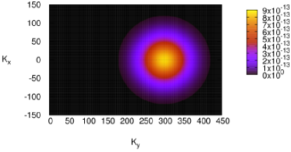
Figure 1: Initial spectrum $|a_{\vec{k}}|^{2}$. $t=0$.

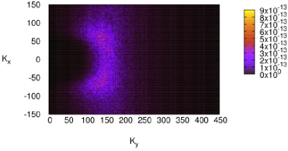
Figure 2: Final spectrum $|a_{\vec{k}}|^{2}$. $t\simeq 2809T_{0}$.

We observed the following indications of wave-turbulent behavior:

1. The statistics of energy-capacity spectral modes is close to the Rayleigh distribution. We observed the presence of a few very intensive harmonics (so-called oligarchs, cf. ZKPD2005 ), which did not obey the Rayleigh statistics, but their contribution to the total balance of the wave action is small (no more than $5\%$). This means that we almost overcame negative effects caused by the finite size of our system (see ZKPD2005 ; LNP2006 ; Nazarenko2006 ), and that our grid is fine enough.

2. We observed the formation of the Zakharov-Filonenko spectral tail in the energy spectrum $|\eta_{\omega}|^{2}$ (see Fig. 3).

Figure 3: The time-averaged spectrum of a point on the surface $n_{\omega}=\langle|\eta_{\omega}|^{2}\rangle$ in the double logarithmic scale. The tail of the distribution fits to the Zakharov-Filonenko spectrum $\omega^{-4}$.

At the same time, we observed a manifestation of strong-turbulent effects. They are manifested by the formation of “fat tails” on the PDF for surface elevations and especially for its gradients (see Fig.4)

Figure 4: PDF for $(\nabla\eta)_{y}$ at the moment of the maximum surface roughness. $t\simeq 14T_{0}$.

The presence of these tails indicates that the surface has a tendency to become rough and to produce white-capping. In our model, wave-breaking is arrested by the strong pseudo-viscosity.

III Statistical experiments

In the second experiment, we solved the Hasselmann kinetic equation for $n_{\vec{k}}=\langle|a_{\vec{k}}|^{2}\rangle$ Hasselmann1962

$$\begin{array}[]{l}\displaystyle\frac{\partial n_{\vec{k}}}{\partial t}=S_{nl}[n]+S_{diss}+2\gamma_{k}n_{\vec{k}},\\ \displaystyle S_{nl}[n]=2\pi g^{2}\int|T_{\vec{k},\vec{k}_{1},\vec{k}_{2},\vec{k}_{3}}|^{2}\left(n_{\vec{k}_{1}}n_{\vec{k}_{2}}n_{\vec{k}_{3}}+\right.\\ \displaystyle\left.+n_{\vec{k}}n_{\vec{k}_{2}}n_{\vec{k}_{3}}-n_{\vec{k}}n_{\vec{k}_{1}}n_{\vec{k}_{2}}-n_{\vec{k}}n_{\vec{k}_{1}}n_{\vec{k}_{3}}\right)\times\\ \displaystyle\times\delta\left(\omega_{k}+\omega_{k_{1}}-\omega_{k_{2}}-\omega_{k_{3}}\right)\times\\ \displaystyle\times\delta\left(\vec{k}+\vec{k}_{1}-\vec{k}_{2}-\vec{k}_{3}\right)\,\mathrm{d}\vec{k}_{1}\mathrm{d}\vec{k}_{2}\mathrm{d}\vec{k}_{3}.\end{array}$$ (5)

Here $\gamma_{k}$ is the pseudo-viscosity and $S_{diss}$ is the phenomenological dissipation term modelling the white-capping process.

Eq. (5) was solved on the grid $71\times 36$ in polar coordinates on the frequency-angle plane by the Resio-Tracy code RT1982 , improved in Zakharov2005 ; BPRZ2005 . We first performed the experiment with $S_{diss}=0$. We observed good qualitative coincidence with the dynamical experiment. We observed a downshift of the spectral peak, angular spreading and the formation of $\omega^{-4}$ spectral tails. But the quantitative agreement of the experiments was not good: it was clear that the inclusion of some phenomenological dissipation is necessary.

We examined the standard from of $S_{diss}$ used in in the industrial operational models of wave forecasting — WAM Cycle 3 and WAM Cycle 4 (hereafter WAM3 and WAM4) SWAN :

$$S_{diss}=C_{ds}\tilde{\omega}\frac{k}{\tilde{k}}\left((1-\delta)+\delta\frac{k}{\tilde{k}}\right)\left(\frac{\tilde{S}}{\tilde{S}_{pm}}\right)^{p}n_{k}$$ (6)

where $k$ and $\omega$ are the wave number and the frequency, tilde denotes the mean value; $C_{ds}$, $\delta$ and $p$ are tunable coefficients; $S=\tilde{k}\sqrt{H}$ is the overall steepness; $\tilde{S}_{PM}=(3.02\times 10^{-3})^{1/2}$ is the value of $\tilde{S}$ for the Pierson-Moscowitz spectrum (note that the characteristic steepness is $\mu\simeq\sqrt{2}S$). It is worth noting that according to BBY2000 , the theoretical value of the steepness for the Pierson-Moscovitz spectrum is $S_{PM}\simeq(4.57\times 10^{-3})^{1.2}$, which gives us $\mu\simeq 0.095$.

The values of tunable coefficients in the WAM3 case are:

$$C_{ds}=2.36\times 10^{-5},\,\,\,\delta=0,\,\,\,p=4$$ (7)

and in the $WAM4$ case are:

$$C_{ds}=4.10\times 10^{-5},\,\,\,\delta=0.5,\,\,\,p=4$$ (8)

The evolution of the total wave action is presented on Fig. 5. One can see that in the long run, the models WAM3 and WAM4 overestimate white-capping dissipation. To achieve better agreement of both experiments, we used the following form of the dissipative term:

$$C_{ds}=1.00\times 10^{-6},\,\,\,\delta=0,\,\,\,p=12$$ (9)

The total wave action curve corresponding to this new dissipation term is shown on Fig. 5 by the thick solid line and displays excellent correspondence with the dynamical model.

Figure 5: Total wave action as a function of time. The solid line corresponds to the dynamical equations, the dashed-dotted line — to the kinetic equation with artificial viscosity, the dashed line — to the kinetic equation with the WAM3 damping term, the dotted line — to the kinetic equation with the WAM4 damping term, and the thick solid line — to the kinetic equation with the new damping term,

IV Conclusion

Our experiments can be interpreted as a confirmation of the theory of weak turbulence. However, even at moderate values of the parameter of the nonlinearity $\mu$, the strongly nonlinear effects of white-capping are essential. They manifest themselves as fat tails of the $PDF$ and lead to additional dissipation of wave energy. This dissipation demonstrates a very strong dependence on the steepness. At steepness $\mu=0.176$ they dominate, at steepness $\mu=0.09$ they are negligibly small. The results of our experiments are in good qualitative agreement with the field experiment of Banner, Babanin and Young BBY2000 , who found that wave-breaking is a threshold effect, similar to a second-order phase transition.

We stress that the dependence (9) is much sharper than it is usually stated. So far, the sharpest dependence $p=5$ was given by Donelan Donelan2001 . We can guess that the real dependence of $S_{diss}$ on $\mu$ is even stronger, and that the onset of the wave breaking is a threshold-type phenomenon like a second-order phase transition.

V Acknowledgments

This work was partially supported by ONR grant N00014-03-1-0648, US Army Corps of Engineers grant DACW 42-03-C-0019 and by NSF grant NDMS0072803, RFBR grant 06-01-00665-a, INTAS grant 00-292, the Program “Nonlinear dynamics and solitons” from the RAS Presidium and “Leading Scientific Schools of Russia” grant NSh-7550.2006.2. A.O. Korotkevich was also supported by the Russian President grant for young scientists MK-1055.2005.2.

The authors would also like to thank the creators of the open-source fast Fourier transform library FFTW FFTW for this fast, portable and completely free piece of software.

References

- (1) L.W. Nordheim, Proc.R.Soc., A 119, 689 (1928).
- (2) R. Peierls, Ann. Phys. (Leipzig), 3, 1055 (1929).
- (3) K. Hasselmann, J.Fluid Mech., 12, 48, 1 (1962).
- (4) V. E. Zakharov, G. Falkovich, and V. S. Lvov, Kolmogorov Spectra of Turbulence I (Springer-Verlag, Berlin, 1992).
- (5) V. E. Zakharov, Nonlin. Proc. Geophys., 12, 1011 (2005).
- (6) S. I. Badulin, A. Pushkarev, D. Resio and V. E. Zakharov, Nonlin. Proc. Geophys., 12, 891 (2005).
- (7) A. I. Dyachenko, A. C. Newell, A. Pushkarev and V. E. Zakharov, Physica D 57, 96 (1992).
- (8) F. Dias, A. Pushkarev and V. E. Zakharov, Physics Reports, 398, 1 (2004).
- (9) V. E. Zakharov, J. Appl. Mech. Tech. Phys. 2, 190 (1968).
- (10) V. E. Zakharov, Eur. J. Mech. B/Fluids, 18, 327 (1999).
- (11) V. E. Zakharov and N. N. Filonenko, Doklady Acad. Nauk SSSR, 160, 1292 (1966).
- (12) M. L. Banner, A. V. Babanin, I. R. Young, J. Phys. Oceanogr., 30, 3145 (2000).
- (13) A. N. Pushkarev and V. E. Zakharov, Phys. Rev. Lett. 76, 18, 3320 (1996).
- (14) A. N. Pushkarev, European Journ. of Mech. B/Fluids 18, 3, 345 (1999).
- (15) A. N. Pushkarev and V. E. Zakharov, Physica D 135, 98 (2000)
- (16) M. Tanaka, Fluid Dyn. Res. 28, 41 (2001).
- (17) M. Onorato, A. R. Osborne, M. Serio at al., Phys. Rev. Lett. 89, 14, 144501 (2002).
- (18) A. I. Dyachenko, A. O. Korotkevich and V. E. Zakharov, JETP Lett. 77, 10, 546 (2003). arXiv:physics/0308101
- (19) A. I. Dyachenko, A. O. Korotkevich and V. E. Zakharov, Phys. Rev. Lett. 92, 13, 134501 (2004). arXiv:physics/0308099.
- (20) N. Yokoyama, J. Fluid Mech. 501, 169 (2004).
- (21) V. E. Zakharov, A. O. Korotkevich, A. N. Pushkarev and A. I. Dyachenko, JETP Lett. 82, 8, 487 (2005). arXiv:physics/0508155.
- (22) Yu. Lvov, S. V. Nazarenko and B. Pokorni, Physica D 218, 1, 24 (2006). arXiv:math-ph/0507054.
- (23) S. V. Nazarenko, J. Stat. Mech. L02002 (2006). arXiv:nlin/0510054.
- (24) A. I. Dyachenko, A. O. Korotkevich and V. E. Zakharov, JETP Lett. 77, 9, 477 (2003). arXiv:physics/0308100.
- (25) F. Dias, A. I. Dyachenko, and V. E. Zakharov, arXiv:0704.3352 (2007).
- (26) SWAN Cycle III user manual, http://fluidmechanics.tudelft.nl/swan/index.htm
- (27) D. Resio, B. Tracy, Theory and calculation of the nonlinear energy transfer between sea waves in deep water, Hydraulics Laboratory, US Army Engineer Waterways Experiment Station, WIS Report 11 (1982).
- (28) M. A. Donelan, A nonlinear dissipation function due to wave breaking. Proc. ECMWF Workshop on ocean wave forecasting, Reading, United Kingdom, ECMWF, 87-94 (2001).
- (29) http://fftw.org, M. Frigo and S. G. Johnson, Proc. IEEE 93, 2, 216 (2005).