Coulomb Gas on the Keldysh Contour: Anderson-Yuval-Hamann representation of the Nonequilibrium Two Level System

Abstract

The nonequilibrium tunneling center model of a localized electronic level coupled to a fluctuating two-state system and to two electronic reservoirs, is solved via an Anderson-Yuval-Hamann mapping onto a plasma of alternating positive and negative charges time-ordered along the two “Keldysh” contours needed to describe nonequilibrium physics. The interaction between charges depends both on whether their time separation is small or large compared to a dephasing scale defined in terms of the chemical potential difference between the electronic reservoirs and on whether their time separation is larger or smaller than a decoherence scale defined in terms of the current flowing from one reservoir to another. A renormalization group transformation appropriate to the nonequilibrium problem is defined. An important feature is the presence in the model of a new coupling, essentially the decoherence rate, which acquires an additive renormalization similar to that of the energy in equilibrium problems. The method is used to study interplay between the dephasing-induced formation of independent resonances tied to the two chemical potentials and the decoherence which cuts off the scaling and leads to effectively classical long-time behavior. We determine the effect of departures from equilibrium on the localization-delocalization phase transition.

I Introduction

Understanding the nonequilibrium behavior of interacting quantum mechanical systems is one of the important open issues in condensed matter physics, with applications in nanoscience Paaske06 , the study of cold atoms in optical lattices Morsch06 , nonlinear spectroscopies Axt98 and, transport at quantum critical points Hogan06 . One may distinguish three classes of nonequilibrium situations: response of a system initially in an equilibrium state to a strong transient pulse, time evolution of a system from a particular initial condition, and the steady state behavior of a driven system. In this paper we shall be concerned with one of the simplest examples of the third class of problems: a quantum mechanical system with only a few degrees of freedom, coupled to two reservoirs with which particles and energy may be exchanged, and with the nonequilibrium drive arising from a difference, $\Delta\mu$, in chemical potential $\mu$ between the reservoirs. This model is of experimental relevance in the context of single molecule devices singlemolecule and of quantum dots kondoinquantumdot and is important as a paradigm problem for the development of techniques and insights. Two crucial issues in nonequilibrium physics are dephasing and decoherence. In the model we study dephasing arises because the wave functions in the two reservoirs evolve in time at rates which differ by $\Delta\mu$ whereas decoherence arises from the flow of energy and particles across the system. An important issue in nonequilibrium physics is to develop methods which allow these effects to be systematically analyzed.

On the formal level, investigation of equilibrium systems is based on the partition function. Powerful techniques, most importantly the renormalization group method, enable one to eliminate putatively unimportant degrees of freedom and derive an effective theory governing the low energy behavior of interest. The renormalization group has been implemented in two intimately related ways: by considering changes in the self energies, vertex functions, and correlation functions in diagrammatic calculations, and by working directly with the partition function, generating an effective action describing only the degrees of freedom of interest.

Most applications of renormalization group ideas to nonequilibrium problems have been based on the first approach: a diagrammatics is constructed using the Keldysh technique and then the flow of vertices, self energies and response functions under changes in cutoff is studied. In pioneering work Rosch and co-workers Rosch01 ; Rosch03 constructed a nonequilibrium scaling theory for the Kondo problem by identifying logarithms in perturbative calculations. Measurable quantities are computed, scaling equations for the coupling constants of the Hamiltonian were inferred from logarithmic dependences of observables on the upper frequency cutoff. In a very recent paper Borda et al Borda07 used similar techniques to study the nonequilibrium behavior of the tunneling center model by perturbation theory in the dot-lead coupling. Paaske et. al provided further insight Paaske04a ; Paaske04b into the physically crucial issue of decoherence rates, showing that voltage-induced decoherence enters differently into different observables, so that the analogy between temperature and decoherence is not precise. In a more recent set of approaches, a transformation is performed on the Hamiltonian itself.  Kehrein05 ; Gezzi07

While these approaches have established a number of basic results and concepts, the development of the subject remains incomplete. In equilibrium, defining a renormalization group transformation directly on the free energy provided important insights into the meaning of the transformations and the formal structure of the theory. A similar analysis out of equilibrium should lead to valuable insights including a clearer understanding of decoherence and dissipation and a more precise definition of the charges in the renormalization group equations and the ability to map one problem onto another. In this paper we therefore examine a simple model, the tunneling center problem, from the effective action point of view. The “tunneling center” model is perhaps the simplest example of a wide class of quantum impurity models such as the Kondo problem or the spin-boson problem, which involve a finite number of local degrees of freedom coupled to reservoirs. The equilibrium behavior of these models is very rich, involving nontrivial correlated states, dynamically generated energy scales and quantum phase transitions TLS . The equilibrium physics revolves around a competition between formation of a quantum coherent state of the local degrees of freedom and the decoherence associated with coupling to the reservoir. We wish to characterize the effect of departures from equilibrium on this physics.

Effective actions for nonequilibrium problems have been discussed by several authors; for a review see e.g. Kamenev04 . Here we define and analyze a renormalization group transformation directly on the effective action. Our approach is somewhat similar to previous work of König and collaborators, Konig96 ; Konig00 who defined a renormalization group transformation directly on the equation of motion for the density matrix. These authors treated the dot-lead coupling via (self-consistently resummed) perturbation theory. We study a simpler model in which we are able to treat the dot-lead coupling exactly. Our formalism allows us to deal with decoherence and orthogonality physics on the same footing. We show that the dephasing scale $\Delta\mu$ defines a crossover beyond which both the physics and the formalism changes. We find that the effective theory valid for energy scales lower than $\Delta\mu$ is characterized by a richer structure of charges than is the corresponding equilibrium theory. It also involves, as a new parameter, a decoherence rate. This arises physically from the flow of current through the system. It enters the theory as an additional parameter, which is subject to additive renormalization (as is the total energy in usual RG treatments). This is discussed in more detail in section III.

The rest of the paper is organized as follows. In section  II we define the model we consider and obtain the effective action. In section III we derive the relevant scaling equation, and in section IV we present the solution and its physical content, among other things displaying the different physics of decoherence and dephasing. Section V is a summary and conclusion, which outlines implications for other problems.

Figure 1: Sketch of energy levels and cutoffs; band energy cutoffs chosen for each lead to be symmetrical about Fermi energy in that lead. (A) (upper panel): chemical potential difference $\Delta\mu=\mu_{L}-\mu_{R}=0$. (B) (middle panel) Chemical potential difference $\Delta\mu\neq 0$ but less than cutoff $2\xi^{-1}$. (C) (lower panel) Chemical potential difference $\Delta\mu$ greater than cutoff $2\xi^{-1}$; no dissipation processes possible.

II Model and derivation of the Coulomb gas

There are many realizations of the tunneling center model SBexamples . We consider a two-state system, which we represent in spin notation, linearly coupled to the density of electrons in an N-fold degenerate electronic level (creation operator $d^{\dagger}_{\alpha}$ with $\alpha=1...N$), which is itself hybridized with two ($L$ and $R$) leads characterized by free-fermion statistics with possibly different chemical potentials i.e., $\Delta\mu=\mu_{L}-\mu_{R}\neq 0$. We consider mainly temperature $T=0$. We assume that the coupling to the leads preserves the “pseudospin” index $\alpha$. The Hamiltonian may then be written as ($S_{z,x}=\frac{1}{2}\sigma_{x,z}$ is a spin matrix)

$$H = H_{loc}+H_{bath}$$ (1)

$$H_{loc} = S_{z}B+\Delta_{T}S_{x}+\lambda DS_{z}\sum_{\alpha=1..N}d^{\dagger}_{\alpha}d_{\alpha}$$ (2)

$$H_{bath} = \sum_{a=L,R,\alpha=1..N}\int d\epsilon\frac{\epsilon}{D}c_{\epsilon a\alpha}^{\dagger}c_{\epsilon a\alpha}+\sqrt{\frac{1}{\pi}}\int d\epsilon\sum_{a=L,R,\alpha=1..N}\left(\cos\theta_{a}c_{\epsilon a\alpha}^{\dagger}d_{\alpha}+h.c.\right)$$

where $0\leq\theta_{L}=\frac{\pi}{2}-\theta_{R}\leq\frac{\pi}{2}$ and we have absorbed the mean hybridization strength into the variable $\varepsilon$. The density of states per pseudospin $\alpha$ in the leads is $D^{-1}$. For the two level system we choose the spin basis which diagonalizes the coupling to the $d$ electrons, and parameterize this coupling by a dimensionless variable $\lambda$ and the lead density of states. The “magnetic field” $B$ is the level splitting of the two level system and the parameter $\Delta_{T}$ gives the tunneling between the states. Note that if $B=0$ the Hamiltonian has a particle-hole symmetry, so its energies are invariant under combined operations of changing the state of the two level system from “up” to “down” and changing particles to holes ($d\leftrightarrow d^{\dagger}$); this simplifies the algebra without changing the conclusions.

The model requires an upper cutoff, $\xi^{-1}$ for the energy integrals. It is most convenient to assume that in each lead the cutoff is symmetrical about the chemical potential in that lead, i.e. in lead $a$ the energy integrals run from $\mu_{a}-\xi^{-1}$ to $\mu_{a}+\xi^{-1}$ (see Fig. 1). We assume that in the starting model the cutoff energies are much larger than the chemical potential difference or than the level splitting parameter $B$.

Crucial parameters of the model are the nonequilibrium phase shifts introduced in Ng96 and defined by

$$\delta_{a}=\arctan{\left[\frac{\lambda\cos^{2}\theta_{a}}{1-\frac{\lambda^{2}}{4}-isgn(\mu_{a}-\mu_{\bar{a}})\lambda\sin^{2}\theta_{a}}\right]}$$ (4)

Note that the phase-shifts are not independent variables, but are related to each other as $\delta_{eq}=\delta_{L}+\delta_{R}=\arctan\lambda/(1-\lambda^{2}/4)$. Also note that while $\delta_{eq}$ is just the difference of the equilibrium phase shifts $\pm\tan^{-1}\frac{\lambda}{2}$ associated with the two states $S_{z}=\pm\frac{1}{2}$, $\delta_{L,R}$ are not the differences of the nonequilibrium phase shifts associated with the two states.

The behavior of the two level system is specified by the reduced density matrix, given at time $t$ in terms of an initial condition $\rho(0)$ at time $t=0$ by

$$\hat{\rho}_{S}=Tr_{el}\left[e^{-iHt}\rho(0)e^{iHt}\right]$$ (5)

Here $Tr_{el}$ indicates a trace over all of the electronic degrees of freedom. We follow Anderson, Yuval and Hamann Anderson69 and expand $\hat{\rho}_{S}$ perturbatively in the “spin-flip” amplitude $\Delta_{T}$. The spin flip events are viewed as particles with “fugacity” $ln\left[\xi\Delta_{T}\right]$ and interaction determined by the trace over electrons. The new features are the need for two time contours and a dependence of the interaction on the chemical potential difference $\Delta\mu$.

A term in the expansion of the density matrix consists of $n_{-}$ spin-flip events at times running from $0_{-}$ to $t$ along the time-ordered contour, followed by $n_{+}$ anti-time-ordered from $t$ to $0_{+}$. Some examples are shown on the left side of Fig 2: the top panel has $n_{+}=4$, $n_{-}=0$ whereas in the two lower panels $n_{+}=n_{-}=2$. Labeling the times in this “Keldysh order” (time ordered on the $-$ contour and anti-time ordered on the $+$ contour) we have for the diagonal components of the density matrix ($\sigma=\pm 1$ below represents the state of the impurity spin),

$$\langle\sigma|\hat{\rho}_{S}(t)|\sigma\rangle =\sum_{n_{-}+n_{+}=even}(-i)^{n_{-}}i^{n_{+}}\langle\sigma|\tau_{x}^{n_{-}}\rho_{S0}\tau_{x}^{n_{+}}|\sigma\rangle$$

$$\left[\int_{0}^{t}\frac{dt_{n_{-}}}{\xi}\int_{0}^{t_{n_{-}}}\frac{dt_{n_{-}-1}}{\xi}\ldots\int_{0}^{t_{2}}\frac{dt_{1}}{\xi}\right]\left[\int_{0}^{t}\frac{dt_{n_{-}+1}}{\xi}\int_{0}^{t_{n_{-}+1}}\frac{dt_{n_{-}+2}}{\xi}....\int_{0}^{t_{n_{-}+n_{+}-1}}\frac{dt_{n_{+}+n_{-}}}{\xi}\right]$$

$$\left(\Delta_{T}\xi\right)^{n_{-}+n_{+}}\exp\left[I_{0}(\{t_{k}\})\right]$$

The interaction $I_{0}$ is obtained by evaluating the $Tr_{el}$, in other words by solving the Keldysh problem of electrons in the time dependent potential specified by the spin flips. In principle this is a multiparticle interaction depending on all of the times $\{t_{k}\}$. In the equilibrium problem an essentially complete analytical solution exists Anderson69 , showing that the interaction is pairwise, with a logarithmic time dependence and coefficients given by the product of the sign of the charges (i.e. whether the spin flips from up to down) and the changes in scattering phase shifts. In the nonequilibrium case general analytical expressions are not known. The available evidence, including solutions at times short and long compared to $\Delta\mu$, perturbative calculations mitra06 and numerics segal06 suggests the following structure, which is slightly more involved than in equilibrium.

To specify the structure, it is convenient to collapse the two-contour problem onto a single time axis by defining classical ($V_{cl}=\frac{\lambda D}{2}\{S_{z}(t_{-})+S_{z}(t_{+})\}$) and quantum fields ($V_{q}=\frac{\lambda D}{2}\{S_{z}(t_{-})-S_{z}(t_{+})\}$). We then have a four state system, in which either $V_{q}=0$ and $V_{cl}=\pm\lambda D/2$ or $V_{cl}=0$ and $V_{q}=\pm\lambda D/2$. Transitions between these states are instantons, which we label by an integer $n=\pm 1$ giving the sign of the change in the quantum field (this is just the usual Coulomb gas charge) and an integer $q=\pm 1$ corresponding to the sign of the quantum field in the region where it is non-zero. The right hand panels of Fig 2 show some examples.

There are in principle 16 pairwise interactions between the 4 kinds of instantons, but calculations reveal a simpler structure (see Appendix $A$). We find that the interaction between instantons at times $t_{i}$ and $t_{j}$ is pairwise, as in equilibrium. As in equilibrium the sign of the interaction between instantons $i$ and $j$ is determined in the usual way by the product of the charges $n_{i}n_{j}$, while the magnitude is determined by the product of the scattering phase shifts. However in the general nonequilibrium case the phase shifts are complex and take value $\delta_{i}$ if $q_{i}=1$ and $\delta^{*}_{i}$ if $q_{i}=-1$ (see Appendix $A$). Finally, with each interaction is a phase factor. The interaction has a logarithmic time dependence, given approximately by $ln\frac{ia_{ij}|t_{i}-t_{j}|+\xi}{\xi}$, with phase factor $a_{ij}=\pm 1$ determined by the Keldysh time-ordering of $t_{i}$ and $t_{j}$, so that in the upper panel of Fig 2 $a_{23}=1$ whereas in the middle panel $a_{23}=-1$. We find it convenient to combine the phase factors into an over-all phase $\Phi$. The result is

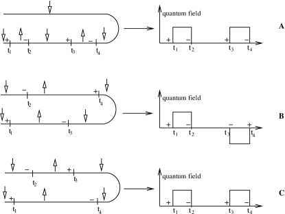
Figure 2: Examples of spin-flip events in the Keldysh two axis representation (left side), and in the single axis representation employing quantum and classical fields (right side). The charges $n_{i}$ are indicated on the Figure. In the top and bottom examples the fields $q=+1$ for all instantons. In the middle example $q=+1$ for the left hand pair of instantons and $=-1$ for the right hand pair. Although the first and the third examples have the same quantum field configuration, but the different positions of the times on the Keldysh contour leads to different phase factors.

$$\langle\sigma|\hat{\rho}_{S}(t)|\sigma\rangle =\sum_{n_{-}+n_{+}=even}(-i)^{n_{-}}i^{n_{+}}\langle\sigma|\tau_{x}^{n_{-}}\rho_{S0}\tau_{x}^{n_{+}}|\sigma\rangle\int_{0}^{t}\frac{dt_{n_{-}+n_{+}}}{\xi}\int_{0}^{t_{n_{-}+n_{+}-1}}\ldots\int_{0}^{t_{2}}dt_{1}\left(\Delta_{T}\xi\right)^{n_{-}+n_{+}}$$

$$\sum^{\prime}_{n_{i},q_{i}v_{i}}\exp\left[\sum_{j<i}n_{i}n_{j}C_{0}(q_{i},q_{j},\frac{t_{i}-t_{j}}{\xi},\Delta\mu\xi)+i\Phi\right]$$

The prime symbol on the sum above is to keep track of constraints such as, two charges of the same sign cannot appear more than twice in sequence, and $\sum_{i}n_{i}=0$ for an expansion involving the diagonal component of the density matrix.

The long Ng96 and short Anderson69 ; Nozieres69 time limits of the interaction function $C_{0}$ are known. At short times $t<1/\Delta\mu$

$$C_{0}(\Delta\mu t\ll 1)=N\left(\frac{\delta_{L}+\delta_{R}}{\pi}\right)^{2}\ln\left(\frac{|t|}{\xi}\right)$$ (8)

independent of quantum fields. At long times $t>\frac{1}{\Delta\mu}$, we have

$$C_{0}(q=+,q=+,\Delta\mu t>1;\Delta\mu\xi\ll 1)(t)=\{C_{0}(q=-,q=-)\}^{*} = N\left(\frac{\delta_{L}^{2}}{\pi^{2}}+\frac{\delta_{R}^{2}}{\pi^{2}}\right)\ln{\left(|\Delta\mu t|\right)}+\Gamma_{neq}|t|$$ (9)

$$+ N\left(\frac{\delta_{L}+\delta_{R}}{\pi}\right)^{2}\left[\ln{\frac{1}{\Delta\mu\xi}}\right]$$

$$C_{0}(q=+,q=-,\Delta\mu t>1;\Delta\mu\xi\ll 1)(t)=C_{0}(q=-,q=+) = N\left(\frac{|\delta_{L}|^{2}}{\pi^{2}}+\frac{|\delta_{R}|^{2}}{\pi^{2}}\right)\ln{\left(|\Delta\mu t|\right)}+\Gamma_{neq}|t|$$ (10)

$$+ N\left(\frac{\delta_{L}+\delta_{R}}{\pi}\right)^{2}\left[\ln{\frac{1}{\Delta\mu\xi}}\right]$$

From Eqns. 9 and  10, note that the dynamics is characterized by an exponential time decay, which we use to define the decoherence rate $\Gamma_{neq}$ which plays a fundamental role in the subsequent analysis:

$$\Gamma_{neq}=\gamma_{neq}\Delta\mu=N\Delta\mu\frac{|\delta_{L}^{\prime\prime}-\delta_{R}^{\prime\prime}|}{2\pi}=N\Delta\mu\xi\left(\frac{1}{\pi}\lambda^{2}\cos^{2}\theta_{L}\sin^{2}\theta_{L}+\ldots\right).$$ (11)

.

The physics expressed by the interaction $C_{0}$ in the $\Delta\mu\xi\ll 1$ limit is as follows: for times less than the dephasing scale $t_{dephasing}=(\Delta\mu)^{-1}$ one has the equilibrium result: the two level system interacts with one coherent combinations of the two leads ($\bar{c}^{\dagger}=\cos\theta_{L}c_{L}^{\dagger}+\sin\theta_{R}c_{R}^{\dagger}$); the other combination decouples. The coupling leads to the usual power law interaction with exponents given by the coherent phase shift $\delta_{eq}=\delta_{L}+\delta_{R}$. Note that $\delta_{eq}$ is independent of quantum fields. For times longer than the dephasing scale, one has a richer structure. The model is effectively a two channel model with separate couplings to left and right leads. The interaction between instantons acquires a dependence on the quantum field. At times longer than the decoherence scale $\Gamma_{neq}^{-1}$ the interaction is cut off altogether.

These limiting forms suggest the following decomposition of the interaction:

$$C_{0}(q,q^{\prime},t-t^{\prime},\Delta\mu,\xi)=Q_{0}(q,q^{\prime})h_{0}\left(\frac{t-t^{\prime}}{\xi}\right)+Q_{M}(q,q^{\prime})h_{M}\left(\frac{t-t^{\prime}}{\xi},\Delta\mu(t-t^{\prime})\right)+\gamma_{neq}h_{neq}\left(\frac{t-t^{\prime}}{\xi},\Delta\mu(t-t^{\prime})\right)$$ (12)

where the “charges” or phase shifts $Q_{0,M}$ obey the property

$$Q_{0,M}(q,q^{\prime})=\left[Q_{0,M}(-q,-q^{\prime})\right]^{*}$$ (13)

$$Q_{0,M}(q,-q)=Q_{0,M}(-q,q)=>Im[Q_{0,M}(q,-q)]=0$$ (14)

The precise form of the functions $h_{0,M,neq}$ depend on the cutoff scheme, but for $t/\xi\gg 1$ and $\Delta\mu\xi\ll 1$ (see Appendix  B)

$$h_{0}(t/\xi) = \ln(|t|/\xi)$$ (15)

$$h_{M}(t/\xi,\Delta\mu t) = h_{0}(t/\xi),\,\,\,\,\,\,\Delta\mu t\ll 1$$ (16)

$$= \ln\frac{1}{\Delta\mu\xi},\,\,\,\,\,\,\Delta\mu t\gg 1$$ (17)

$$h_{neq}(t/\xi,\Delta\mu t) = \frac{2}{\pi}(\Delta\mu t)^{2},\,\,\,\,\,\,\Delta\mu t\ll 1$$ (18)

$$= |\Delta\mu t|,\,\,\,\,\,\,\Delta\mu t\gg 1$$ (19)

implying that for a model with $\Delta\mu\xi\ll 1$,

$$Q_{0}(+,+)=N(\frac{\delta_{L}^{2}}{\pi^{2}}+\frac{\delta_{R}^{2}}{\pi^{2}})$$ (20)

$$Q_{M}(+,+)=\frac{2N}{\pi^{2}}\delta_{L}\delta_{R}$$ (21)

$$Q_{0}(+,-)=N(\frac{\delta_{L}\delta_{L}^{*}}{\pi^{2}}+\frac{\delta_{R}\delta_{R}^{*}}{\pi^{2}})$$ (22)

$$Q_{M}(+,-)=N\frac{\delta_{L}\delta_{R}^{*}+\delta_{R}\delta_{L}^{*}}{\pi^{2}}$$ (23)

The coefficient $\gamma_{neq}$ is independent of the quantum fields and is given by

$$\gamma_{neq}=N\frac{|\delta_{L}^{\prime\prime}-\delta_{R}^{\prime\prime}|}{2\pi}$$ (24)

The first term proportional to $Q_{0}$ in Eq 12 represents the effect of processes in which an electron emerges from one lead and is scattered back into the same lead; it is independent of $\Delta\mu$. The term proportional to $Q_{M}$ represents the effect of processes in which an electron is transferred from one lead to another; it depends on $\Delta\mu$. Finally, as will be seen, the last term expresses the decoherence; it vanishes if the coupling is only to one lead.

It is also interesting to consider the expression for $C_{0}$ in a model in which $\Delta\mu\xi>1$. This situation arises after rescaling. In this case the regime $\Delta\mu t<1$ is not defined, and for all times $t>\xi^{-1}$ we find,

$$C_{0}(q=+,q=+,\Delta\mu t>1)=Q_{0}\left[\ln{\frac{|t|}{\xi}}\right]$$ (25)

with (for the model with $\Delta\mu\xi>1$) $Q_{M}=0$ and

$$Q_{0}\rightarrow Q_{0}^{\prime}=\left(\frac{\tan^{-1}{\frac{\lambda\cos^{2}\theta_{L}}{1-\frac{\lambda^{2}}{4}}}}{\pi}\right)^{2}+\left(\frac{\tan^{-1}{\frac{\lambda\cos^{2}\theta_{R}}{1-\frac{\lambda^{2}}{4}}}}{\pi}\right)^{2}$$ (26)

In this limit there is no decay because the theory has no real process which allows nonconservation of energy (see Fig. 1, case $C$).

Comparison of Eqs 9 and 25 reveals an important point. If we apply the usual renormalization process of reducing bandwidth we must pass from the model which gives rise to Eq 9 and contains decoherence to the model which gives rise to Eq 25. No decoherence processes exist in this latter model, but the renormalization maps one model onto another model with the same physical content. We therefore conclude that one consequence of renormalization must be the generation of a decay rate, which appears as an extra parameter, additional to what is directly computed from the small bandwidth model.

III Derivation of scaling equations

In the formulation given in Eq. II, the nonequilibrium two level system is seen to be a function of the dimensionless parameters $\Delta_{T}\xi$, $\Delta\mu\xi$ and $\delta_{L,R}$. In this section we construct a renormalization group analysis by following the usual procedure of reducing the energy cutoff, i.e. increasing the time cutoff from $\xi$ to $\xi^{\prime}=(1+\Lambda)\xi$, integrating out the degrees of freedom in the eliminated interval and determining the consequences for the remaining degrees of freedom. These effects were considered for the equilibrium problem by Anderson69 : reducing the energy cutoff (increasing the time cutoff) leads to changes arising from the $\xi$ dependence of $C_{0}$. Rescaling leads to the simple “engineering dimension” changes $(\Delta_{T},\Delta\mu)\rightarrow(\Delta_{T},\Delta\mu)(\xi/\xi^{\prime})\approx(\Delta_{T},\Delta\mu)(1-\Lambda)$. Finally, some kink-antikink pairs fall within the time interval between $\xi$ and $\xi(1+\Lambda)$ and must therefore be removed from the renormalized theory. The procedure for the nonequilibrium problem is similar to the equilibrium problem, in that in the starting formulation the minimum separation in time between tunneling events is $\xi$. In the rescaled theory, spin flip events separated by time intervals less than $\xi^{\prime}$ cannot explicitly appear, but their presence will lead to a renormalization of the interaction between the processes which do explicitly appear in the theory. For small $\Delta_{T}\xi\Lambda$ the sequence of close tunneling events which appears with any probability are the “close pairs” shown in Fig. 3. A close pair may lie between two spin-flip events that occur on the same Keldysh axis (example pairs $A$ and $B$ in Fig 3 that lie between spin-flip events $t_{1},t_{2}$), or may lie between spin-flip events on opposite Keldysh axes (examples $C$ and $D$ that lie between spin-flip events $t_{2},t_{4}$). Physically, a close pair corresponds to a dipole, and leads to a screening of the interaction between other spin flip events that may lie on the same Keldysh axis or on different Keldysh axes. Note that we always consider close pairs that lie on the same axis. A close pair with one member on each contour cannot be considered as a dipole; its removal would change the spin state at the final time $t$ or initial time $t=0$.

Figure 3: Scheme for integrating out close pairs.

Mathematically, the calculation is easiest to perform in the collapsed single axis representation in terms of classical and quantum fields. As an example consider Fig. 4. The interaction between the charge at $t_{i}$ and the charge at $t_{k}$ can get renormalized by integrating out eight kinds of close pairs, four of which are nearest neighbors to charge at $t_{i}$, while the other four are nearest neighbors to the charge at $t_{k}$. We show the four close pairs that are nearest neighbors to $t_{i}$ in Fig 4. Close pair I can occur in two ways which have the same quantum field configuration, but different classical field configuration.

The change in the density matrix, on integrating out the four close pairs is (${\bar{\Delta}}_{T}=i\Delta_{T}\xi$)

$$\rho^{2n+2}=\rho^{2n}\left[1+\bar{\Delta}_{T}^{2}\left(2*I+II+III\right)\right]$$ (27)

Summing over all possible positions of the relative separation $\epsilon$ between the two charges of the close pair, and their center of mass position $\tau$ one obtains,

$$I=\int_{t_{i-1}}^{t_{i}}\frac{d\tau}{\xi}\int_{\xi}^{\xi(1+\Lambda)}\frac{d\epsilon}{\xi}\exp{\left[-C_{0}(+,+,\epsilon)+\sum_{k}n_{i}n_{k}\left(-C_{0}(+,q_{k},|t_{k}-\tau-\frac{\epsilon}{2}|)+C_{0}(+,q_{k}|t_{k}-\tau+\frac{\epsilon}{2}|)\right)\right]}$$ (28)

$$II=\int_{t_{i}}^{t_{i+1}}\frac{d\tau}{\xi}\int_{\xi}^{\xi(1+\Lambda)}\frac{d\epsilon}{\xi}\exp{\left[-C_{0}(+,+,\epsilon)+\sum_{k}n_{i}n_{k}\left(C_{0}(+,q_{k},|t_{k}-\tau-\frac{\epsilon}{2}|)-C_{0}(+,q_{k}|t_{k}-\tau+\frac{\epsilon}{2}|)\right)\right]}$$ (29)

$$III=\int_{t_{i}}^{t_{i+1}}\frac{d\tau}{\xi}\int_{\xi}^{\xi(1+\Lambda)}\frac{d\epsilon}{\xi}\exp{\left[-C_{0}(-,-,\epsilon)+\sum_{k}n_{i}n_{k}\left(-C_{0}(-,q_{k},|t_{k}-\tau-\frac{\epsilon}{2}|)+C_{0}(-,q_{k}|t_{k}-\tau+\frac{\epsilon}{2}|)\right)\right]}$$ (30)

In the above three expressions, the first term in the argument of the exponent represents the self interaction of the close pair, and the second term represents the interaction of the close pair with all other charges. The latter may be Taylor expanded in $\epsilon$. The term I on Taylor expansion takes the form

$$I\sim\int_{t_{i-1}}^{t_{i}}\frac{d\tau}{\xi}\int_{\xi}^{\xi(1+\Lambda)}\frac{d\epsilon}{\xi}e^{-C_{0}(+,+\epsilon)}\left(1-\epsilon\sum_{k}n_{i}n_{k}\frac{\partial C_{0}(|t_{k}-\tau|)}{\partial\tau}\right)$$ (31)

The integrals over $\tau$ and $\epsilon$ can easily be performed. The result is of $O(\Lambda)$, which implies that the change to the density matrix in Eq. 27 is $O(\bar{\Delta}_{T}^{2}\Lambda)\ll 1$, and therefore can be re-exponentiated. Finally, integrating out the four close pairs of Fig 4 leads to the following renormalization of the density matrix,

$$\rho^{2n+2}=\rho^{2n}e^{\bar{\Delta}_{T}^{2}e^{-C_{0}(\xi)}\Lambda(\frac{-2t_{i-1}+2t_{i+1}}{\xi})}$$ (32)

$$e^{\Lambda\bar{\Delta}_{T}^{2}e^{-C_{0}(\xi)}\sum_{k}n_{i}n_{k}\left[-2C_{0}(+,q_{k},|t_{k}-t_{i}|)+2C_{0}(+,q_{k},|t_{k}-t_{i-1}|)+C_{0}(+,q_{k},|t_{k}-t_{i+1}|)-C_{0}(+,q_{k},|t_{k}-t_{i}|)-C_{0}(-,q_{k},|t_{i+1}-t_{k}|)+C_{0}(-,q_{k},|t_{k}-t_{i}|)\right]}$$

Note that the term $e^{-C_{0}(\xi)}$ is from the self-interaction of the close pair. Since this term arises at short times $t\sim\xi$, it has no explicit quantum field dependence, and therefore the quantum field label has been dropped.

Repeating the above computation for all possible positions of close pairs, one finds that the initial factor of $e^{\bar{\Delta}_{T}^{2}e^{-C_{0}(\xi)}\Lambda(\frac{2t_{i+1}-2t_{i-1}}{\xi})}$ cancel among each other, while the function $C_{0}(q_{i},q_{k},|t_{k}-t_{i}|)$ is renormalized in the following way

$$C_{0}(q_{i},q_{k},|t_{k}-t_{i}|)\rightarrow C_{0}(q_{i},q_{k},|t_{k}-t_{i}|)$$ (33)

$$-\Lambda\bar{\Delta}_{T}^{2}\left[6C_{0}(q_{i},q_{k},|t_{k}-t_{i}|)-C_{0}(-q_{i},q_{k},|t_{k}-t_{i}|)-C_{0}(q_{i},-q_{k},|t_{k}-t_{i}|)\right]e^{-C_{0}(\frac{t}{\xi}=1)}$$

Note that $C_{0}(t/\xi=1)=0$ if $\Delta\mu\xi<<1$ but $=\Gamma_{neq}\xi$ if $\Delta\mu\xi>1$.

Figure 4: Close pairs that are nearest neighbors to charge at time $t_{i}$

The second effect arises from the explicit dependence of the interaction $C_{0}$ on the cutoff $\xi$. We write, for infinitesimal $\Lambda$,

$$C_{0}(t,\xi,\Delta\mu)=C_{0}(\frac{t}{\xi^{\prime}},\Lambda\Delta\mu t)+\delta C_{0}$$ (34)

with

$$\delta C_{0}=\frac{dC_{0}(\frac{t}{\xi},\Delta\mu t)}{dln\xi}$$ (35)

Adding Eqns 33 and 34 leads to the fundamental scaling equation,

$$\frac{dC_{0}(q,q^{\prime},t)}{d\ln\xi}=-\bar{\Delta}_{T}^{2}e^{-C_{0}(1)}\left[6C_{0}(q,q^{\prime},t)-C_{0}(-q,q^{\prime},t)-C_{0}(q,-q^{\prime},t)\right]+\frac{dC_{0}(q,q^{\prime},t/\xi,\Delta\mu\xi)}{d\ln\xi}$$ (36)

The second term in Eq. 36 may be computed from the fundamental Eq. 68. While a precise general expression is not known, the limits are established. For $\Delta\mu\xi\ll 1$, Eqns. 9 and 10 show that $\frac{dC_{0}}{d\ln\xi}$ is independent of time, with coefficient $Q_{0}+Q_{M}$ independent of quantum fields. This is just the equilibrium scaling. For $\Delta\mu\xi\gg 1$, Eq. 25 shows that $\frac{dC_{0}}{d\ln\xi}$ is again independent of time, with some coefficient $Q_{0}$ derived from scaling and not, in general, given by Eq. 26. The regime $\Delta\mu\xi\sim 1$ requires a more careful treatment. Differentiation of the perturbative results derived in Appendix  B yields two contributions: a function $g_{M}=\frac{dh_{M}}{d\ln\xi}$ which expresses the dephasing crossover by ”turning off” the $Q_{M}$ contribution to $C_{0}$ as $\Delta\mu\xi$ increases through unity, and an additional contribution proportional to $t$ for $\Delta\mu t>1$ which expresses decoherence by cutting off the interaction between instantons. The decoherence term is characterized by a coefficient $g_{neq}=Lt_{t\rightarrow\infty}\left[\gamma_{neq}\frac{1}{t}\frac{dh_{neq}}{d\ln\xi}\right]$. Fig 5 shows $g_{neq}$ calculated from Appendix  B within perturbation theory to ${\cal O}(\lambda^{2})$ and for hard and soft cutoffs. (Note that the hard cutoff model gives rise to oscillations which we have neglected).

In summary, our scaling theory must keep track of the changes in the function $C_{0}$ as the cutoff is changed, but consideration of the short and long time limits shows that the model has effectively six coupling constants: “Coulomb gas charges” $Q_{0}(+,+),Q_{0}(+,-)$ expressing the part of logarithmic interaction between tunneling events involving the same lead, Coulomb gas charges $Q_{M}(+,+),Q_{M}(+,-)$ expressing the part of the logarithmic interaction which depends on coherence between leads, a tunneling amplitude $\Delta_{Tq}$ (which acquire a quantum field dependence labeled by $q$), and the decoherence rate $\Gamma_{neq}$. These are renormalized according to

$$\frac{d\bar{\Delta}_{T\pm}}{d\ln\xi} = \bar{\Delta}_{T\pm}\left[1-\frac{1}{2}\left[Q_{0}(\pm,\pm)+Q_{M}(\pm,\pm)g_{M}(\Delta\mu\xi)\right]\right]$$ (37)

$$\frac{d\Gamma_{neq}(+,+)}{dln\xi} = -4\left[\Gamma_{neq}(+,+)\bar{\Delta}_{T+}^{2}+\frac{1}{2}\left(\Gamma_{neq}(+,+)\bar{\Delta}_{T+}^{2}-\Gamma_{neq}(+,-)\bar{\Delta}_{T-}^{2}\right)\right]e^{-C_{0}(1)}+g_{neq}(\Delta\mu\xi)$$ (38)

$$\frac{d\Gamma_{neq}(-,-)}{dln\xi} = -4\left[\Gamma_{neq}(-,-)\bar{\Delta}_{T-}^{2}+\frac{1}{2}\left(\Gamma_{neq}(-,-)\bar{\Delta}_{T-}^{2}-\Gamma_{neq}(-,+)\bar{\Delta}_{T+}^{2}\right)\right]e^{-C_{0}(1)}+g_{neq}(\Delta\mu\xi)$$ (39)

$$\frac{d\Gamma_{neq}(+,-)}{dln\xi} = -\left[3\Gamma_{neq}(+,-)\bar{\Delta}_{T-}^{2}+3\Gamma_{neq}(-,+)\bar{\Delta}_{T+}^{2}-\Gamma_{neq}(+,+)\bar{\Delta}_{T+}^{2}-\Gamma_{neq}(-,-)\bar{\Delta}_{T-}^{2}\right]e^{-C_{0}(1)}$$ (40)

$$+ g_{neq}(\Delta\mu\xi)$$

$$\frac{dQ_{0,M}(+,+)}{dln\xi} = -4\left[Q_{0,M}(+,+)\bar{\Delta}_{T+}^{2}+\frac{1}{2}\left(Q_{0,M}(+,+)\bar{\Delta}_{T+}^{2}-Q_{0,M}(+,-)\bar{\Delta}_{T-}^{2}\right)\right]e^{-C_{0}(1)}$$ (41)

$$\frac{dQ_{0,M}(+,-)}{dln\xi} = -\left[3Q_{0,M}(+,-)\bar{\Delta}_{T-}^{2}+3Q_{0,M}(-,+)\bar{\Delta}_{T+}^{2}-Q_{0,M}(+,+)\bar{\Delta}_{T+}^{2}-Q_{0,M}(-,-)\bar{\Delta}_{T-}^{2}\right]e^{-C_{0}(1)}$$ (42)

$$\frac{dQ_{0,M}(-,-)}{dln\xi} = -4\left[Q_{0,M}(-,-)\bar{\Delta}_{T-}^{2}+\frac{1}{2}\left(Q_{0,M}(-,-)\bar{\Delta}_{T-}^{2}-Q_{0,M}(-,+)\bar{\Delta}_{T+}^{2}\right)\right]e^{-C_{0}(1)}$$ (43)

Note that in these expressions $C_{0}(1)=\Gamma_{neq}\xi$ for $\Delta\mu\xi\gg 1$ and $=0$ otherwise. The meaning of Eq. 38, 39, 40 is that as the renormalized chemical potential passes through the scale $\Delta\mu\xi=1$ an additive contribution to $\Gamma_{neq}$ is generated.

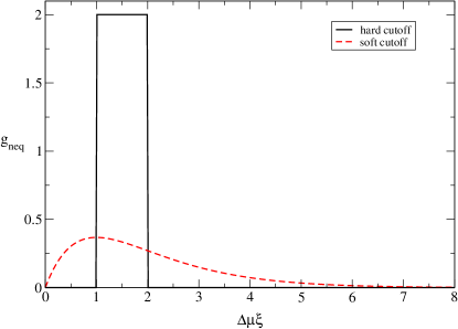
Figure 5: Crossover function $g_{neq}$ (in units of $\frac{\pi}{2}Q_{M}\Delta\mu$) describing additive renormalization of decay constant $\Gamma_{neq}$, for hard (solid line) and soft (dashed line) cutoffs.

IV Solution of the scaling equations

We now discuss the solution of the scaling equations. Notice from Eq. 20 - 23 that in equilibrium ($\Delta\mu=0$), the charges $Q_{0,M}$ are independent of the quantum fields. Moreover out of equilibrium, any explicit dependence on the quantum fields appears to $O(\lambda^{3})$ for asymmetric couplings, and to $O(\lambda^{4})$ for symmetric couplings. We will present results that are valid to $O(\lambda^{2})$, and hence ignore the explicit quantum field dependence of the charges. In this limit, as we shall show, the dominant effect of voltage is due to the decoherence term.

The physically relevant starting point for the solution of the scaling equations is one where the chemical potential difference is small compared to the cutoff scale. In this limit $C_{0}(1),g_{neq}\approx 0$, and $g_{M}(\Delta\mu\xi)\approx 1$; thus the effective Coulomb gas charge $Q=Q_{0}+Q_{M}$ (physically, the level couples to the coherent combination of the leads). The scaling equations thus become

$$\frac{d\bar{\Delta}_{T}}{d\ln\xi} = \bar{\Delta}_{T}\left[1-\frac{Q}{2}\right]$$ (44)

$$\frac{dQ}{dln\xi} = -4Q\bar{\Delta}_{T}^{2}$$ (45)

$$\frac{d\Gamma_{neq}}{dln\xi} = -4\Gamma_{neq}\bar{\Delta}_{T}^{2}$$ (46)

$$\frac{dQ_{M}}{dln\xi} = -4Q_{M}\bar{\Delta}_{T}^{2}$$ (47)

Eqs 44 and 45 are the usual equilibrium scaling equations and are solved as usual; from the solution the behavior of $Q_{M}$ and $\Gamma_{neq}$ is computed. The equations leave the combination $I=\bar{\Delta}_{T}^{2}-\frac{1}{2}(\frac{Q-2}{2}-ln(Q/2))$ invariant. If $I<0$ then the model scales toward $\Delta_{T}=0$ (i.e. is localized) while if $I>0$ then it is on the delocalized side of the phase boundary and $\Delta_{T}$ increases. We discuss the two cases separately.

If the initial conditions are such that the model is on the localized side of the equilibrium phase diagram, then scaling proceeds until the cutoff crosses through the dephasing scale $\Delta\mu\xi=1$. Beyond this point, changes occur. First, the leads decohere: $g_{M}\rightarrow 0$ so the term proportional to $Q_{M}$ drops out of the scaling equations and the charge becomes $Q_{0}$. Depending on the sign of $Q_{M}$ (i.e. the relative sign of $\delta_{R}$ and $\delta_{L}$) this may either make the system more localized or more delocalized. Second, and of greater significance, the decoherence rate $\Gamma_{neq}$ acquires a positive additive term, arising from the function $g_{neq}$ in the scaling equation. Third, the effective coupling becomes $(\bar{\Delta}_{T}^{*})^{2}\equiv\bar{\Delta}_{T}^{2}e^{-C_{0}(1)}\approx\bar{\Delta}_{T}^{2}e^{-\Gamma_{neq}\xi}$. Thus the theory at the scale $\xi>(\Delta\mu)^{-1}$ is characterized by a fugacity $ln\Delta_{T}^{*}\xi$, a decoherence rate $\Gamma_{neq}$, a charge $Q_{0}$, and by the scaling equations

$$\frac{d\bar{\Delta}_{T}}{d\ln\xi} = \bar{\Delta}_{T}\left[1-\frac{Q_{0}}{2}\right]$$ (48)

$$\frac{d\Gamma_{neq}}{dln\xi} = -4\Gamma_{neq}\bar{\Delta}_{T}^{2}e^{-C_{0}(1)}$$ (49)

$$\frac{dQ_{0}}{dln\xi} = -4Q_{0}\bar{\Delta}_{T}^{2}e^{-C_{0}(1)}$$ (50)

We see that scaling proceeds in the usual way until the nonequilibrium scale $\xi=1/\Gamma_{neq}$ is reached; beyond this point the factor $e^{-C_{0}(1)}$ cuts off the scaling and we are left with a perturbative theory.

A particularly important special case occurs if $I=0$. In this case the equilibrium fixed point is $\Delta_{T}=0$, $Q=2$, and if the initial value of $\Delta\mu$ is sufficiently small, this fixed point is approached very closely, so that at the scale $\xi=1/\Delta\mu$

$$\bar{\Delta}_{T}(\xi) = \frac{\bar{\Delta}_{T0}}{1+2\bar{\Delta}_{T0}ln\frac{1}{\Delta\mu\xi_{0}}}\approx\frac{1}{2ln\frac{1}{\xi_{0}\Delta\mu}}$$ (51)

$$Q \approx 2$$ (52)

$$Q_{M} \rightarrow Q_{M}^{*}$$ (53)

Scaling through the crossover region then drives $Q_{M}\rightarrow Q_{M}^{*}$, changes the basic charge to $Q_{0}=2-Q_{M}^{*}$, generates a $\Gamma_{neq}=\frac{\pi}{2}\left|Q_{M}^{*}\right|\Delta\mu$, and does not change $\Delta_{T}$ significantly. Scaling then proceeds until $\xi\rightarrow 1/\Gamma_{neq}\sim 2/(\pi\left|Q_{M}^{*}\right|\Delta\mu$). We therefore see that the dephasing crossover typically shifts the system away from the critical point, and that decoherence then cuts off the scaling. The decoherence cutoff occurs very rapidly, unless $Q_{M}^{*}<<1$, meaning that one of the leads is much more weakly coupled than the other one. In this case a significant nonequilibrium scaling regime can exist.

If the initial condition is on the delocalized side of the equilibrium phase diagram, then again we distinguish two cases, according to whether or not the model flows to strong coupling before $\Delta\mu\xi=1$ or not. In the latter case, the treatment outlined above applies. In the former case, the Kondo or coherence scale is larger than the dissipation rate and a different treatment, beyond the scope of this paper, is needed.

V Conclusions

In this paper we have expressed the nonequilibrium tunneling center model in terms of a Coulomb gas defined on the Keldysh contour. The nonequilibrium problem has a richer structure than the corresponding equilibrium problem. In particular the effective low energy theory is shown to be a Coulomb gas characterized by two parameters (charge and sign of quantum field). Crucial ingredients of the resulting theory are the dephasing arising because the wave functions in the two leads precess at rates which differ by the chemical potential difference, and a decoherence arising from the dissipative processes again allowed when the model is driven out of equilibrium. We showed explicitly that the decoherence effects cut off the power law interaction between instantons which is found at $T=0$ in equilibrium.

Further, we generalized the standard equilibrium scaling theory of the model to the nonequilibrium case. We found that scaling through the dephasing crossover $\Delta\mu\xi\sim 1$ generates an additive renormalization to the decoherence rate. From this we conclude that the decoherence rate is a fundamental parameter of the nonequilibrium theory, which must be explicitly considered in a renormalization process. We further showed explicitly how the decoherence cuts off the renormalization group flow.

A few words on the generalization of this approach to other quantum impurity models, such as the nonequilibrium Kondo model Paaske04a . The key difference between the model studied here and the nonequilibrium Kondo model is the term $\Delta_{T}S_{x}$ in Eq. 2 responsible for spin-flip processes. The analog of $\Delta_{T}S_{x}$ for the Kondo model is $(J_{LL}+J_{RR})(S_{+}s_{-}+h.c.)$ where $S$ is the impurity spin, while $\vec{s}=\sum_{\sigma\sigma^{\prime}kk^{\prime}}\psi^{\dagger}_{k\sigma}\vec{\tau}\psi_{k^{\prime}\sigma^{\prime}}$ are the electron spins which have been written as the following linear combination of the two leads $\psi_{k\sigma}=\frac{\sqrt{J_{LL}}}{\sqrt{J_{LL}+J_{RR}}}c_{k\sigma L}+\frac{\sqrt{J_{RR}}}{\sqrt{J_{LL}+J_{RR}}}c_{k\sigma R}$. Thus in the Anderson-Yuval-Hamann procedure applied to the Kondo model, the $n_{-}+n_{+}$-th order expansion in the spin flip amplitude involves the computation of

$$Tr_{electron}\left[Te^{-i\int_{0}^{t}dt^{\prime}\tilde{V}_{\uparrow}(t^{\prime})}s_{-}(t_{n_{-}})\ldots s_{+}(t_{1})\rho_{S0}^{\uparrow}\tilde{T}e^{+i\int_{0}^{t}dt^{\prime}\tilde{V}_{\uparrow}(t^{\prime})}s_{-}(t_{n_{-}+n_{+}})\ldots s_{+}(t_{n_{-}+1})\right]$$

$$=e^{C_{0}(t_{1},t_{2}\ldots t_{n_{-}+n_{+}})}L(t_{1},t_{2}\ldots t_{n_{-}+n_{+}})$$ (54)

rather than the quantity needed for the model studied in this paper

$$Tr_{electron}\left[Te^{-i\int_{0}^{t}dt^{\prime}\tilde{V}_{\uparrow}}\rho_{S0}^{\uparrow}\tilde{T}e^{+i\int_{0}^{t}dt^{\prime}\tilde{V}_{\uparrow}}\right]=e^{C_{0}(t_{1},t_{2}\ldots t_{n_{-}+n_{+}})}$$ (55)

In equilibrium, the quantity $L$ in Eq. 54 (referred to in the literature as the open line contribution) Nozieres69 acquires the same structure as that of the closed loop part $e^{C_{0}}$, namely that of a Cauchy determinant. Thus Eqns. 54 and Eq. 55 and therefore the Kondo model and the tunneling center model may be related by a simple redefinition of the phase shifts. Out of equilibrium this analysis breaks down because the dephasing between the leads occuring at $\Delta\mu t>1$ gives rise to a two channel structure similar to that analyzed by Fabrizio et al. gogolin and Vladár et al. vlada . A direct numerical evaluation or a mapping to an explicit two channel Kondo model (with decoherence) could be employed.

This work suggests several generalizations. First, the long-time exponential cutoff suggests that a numerical estimation of the perturbation series may be possible. Second, the key issue in seeing a wide nonequilibrium scaling range is to get the decoherence time to be very large compared to the dephasing time. This does not occur naturally in the simple two lead models we have studied. A search for models, involving for example three leads, where this separation of scales occurs more naturally, may be of interest.

Wide classes of models have been studied in equilibrium by Hubbard-Stratonovich methods, in which the partition function is expressed as a sum over configurations of auxiliary fields. In the strong coupling limit of many quantum impurity models a small number of auxiliary field configurations are relevant and the physics is controlled by tunneling between them. Hamann Generalizing this analysis to the nonequilibrium situation is an important open problem mitra06 , for which the methods developed here may be useful. A useful first step might be a comparison to the Bethe-ansatz solvable interacting resonant level model Andrei .

Acknowledgments This work was supported by NSF-DMF 0431350.

Appendix A Derivation of Eq. II

We start from the Hamiltonian in Eq. 1 which we write as a sum of two parts:

$$H = H_{0}+H_{1}$$ (56)

$$H_{0} = S_{z}B+\lambda DS_{z}\sum_{\alpha=1..N}d^{\dagger}_{\alpha}d_{\alpha}+\sum_{a=L,R,\alpha=1..N}\int d\epsilon\frac{\epsilon}{D}c_{\epsilon a\alpha}^{\dagger}c_{\epsilon a\alpha}+\sqrt{\frac{1}{\pi}}\sum_{a=L,R,\alpha=1..N}\int_{\mu_{a}-1/\xi}^{\mu_{a}+1/\xi}d\epsilon\left(\cos\theta_{a}c_{\epsilon a\alpha}^{\dagger}d_{\alpha}+h.c.\right)$$

$$H_{1} = \Delta_{T}S_{x}$$ (57)

When $\Delta_{T}=0$, the Hamiltonian is exactly solvable and represents a noninteracting resonant level hybridized with the leads. The Anderson-Yuval-Hamann approach involves a perturbative expansion in $\Delta_{T}$, treating $H_{0}$ exactly. This procedure was originally carried out for the partition function; we apply it here to the time-dependent density matrix $\rho(t)$ determined from an initial condition $\rho_{0}(t)$ via

$$\rho(t)=e^{-iHt}\rho_{0}e^{iHt}$$ (58)

The reduced density matrix for the impurity spin is defined as

$$\rho_{S}(t)=Tr_{el}\rho(t)$$ (59)

and is a $2\times 2$ matrix whose diagonal elements give the probability of the spin $S$ to be up or down, while the off diagonal elements contain information about phase coherence. Rewriting

$$e^{-iHt}=e^{-iH_{0}t}Te^{-i\int_{0}^{t}dtV(t)}$$ (60)

$$V(t)=e^{iH_{0}t}H_{1}e^{-iH_{0}t}=\Delta_{T}\left[e^{iH_{0}t}S_{x}e^{-iH_{0}t}\right]=\Delta_{T}S_{x}(t)$$ (61)

a perturbative expansion in $V(t)$ of Eq. 59 may be carried out, yielding

$$\hat{\rho}_{S}(t) = \sum_{n_{-},n_{+}}(-i)^{n_{-}}i^{n_{+}}\left(\Delta_{T}\xi\right)^{n_{-}+n_{+}}$$

$$\left[\int_{0}^{t}\frac{dt_{n_{-}}}{\xi}\int_{0}^{t_{n_{-}}}\frac{dt_{n_{-}-1}}{\xi}\ldots\int_{0}^{t_{2}}\frac{dt_{1}}{\xi}\right]\left[\int_{0}^{t}\frac{dt_{n_{-}+1}}{\xi}\int_{0}^{t_{n_{-}+1}}\frac{dt_{n_{-}+2}}{\xi}....\int_{0}^{t_{n_{-}+n_{+}-1}}\frac{dt_{n_{+}+n_{-}}}{\xi}\right]$$

$$Tr_{el}\left[S_{x}(t_{n_{-}})\ldots S_{x}(t_{2})S_{x}(t_{1})\rho_{0}S_{x}(t_{n_{-}+n_{+}})\ldots S_{x}(t_{n_{-}+1})\right]$$

We assume the initial density matrix

$$\rho_{0}=\begin{pmatrix}\rho_{0S}^{\uparrow}\rho^{\uparrow}_{leads}&&0\\ 0&\rho_{0S}^{\downarrow}\rho^{\downarrow}_{leads}\end{pmatrix}$$ (63)

where $\uparrow,\downarrow$ represent the direction of the local impurity spin, while $\rho^{\uparrow/\downarrow}_{leads}$ represents the steady state distribution of the electrons when the local spin is oriented along $\uparrow/\downarrow$. The effect of the spin flip term would be to modify the diagonal components of $\rho_{S}$ from its initial value, and also to introduce off diagonal terms. The perturbative expansion for the diagonal component of $\rho_{S}$ is (note $H_{0}^{\uparrow/\downarrow}$ appearing below implies $H_{0}$ corresponding to $S_{z}=\uparrow/\downarrow$),

$$\langle\uparrow|\rho_{S}|\uparrow\rangle = \sum_{n_{-},n_{+}=0,2,4\ldots}(-i)^{n_{-}}i^{n_{+}}\left(\Delta_{T}\xi\right)^{n_{-}+n_{+}}$$

$$\left[\int_{0}^{t}\frac{dt_{n_{-}}}{\xi}\int_{0}^{t_{n_{-}}}\frac{dt_{n_{-}-1}}{\xi}\ldots\int_{0}^{t_{2}}\frac{dt_{1}}{\xi}\right]\left[\int_{0}^{t}\frac{dt_{n_{-}+1}}{\xi}\int_{0}^{t_{n_{-}+1}}\frac{dt_{n_{-}+2}}{\xi}....\int_{0}^{t_{n_{-}+n_{+}-1}}\frac{dt_{n_{+}+n_{-}}}{\xi}\right]$$

$$Tr_{el}\left[e^{+iH_{0}^{\downarrow}t_{n-}}e^{-iH_{0}^{\uparrow}t_{n-}}\ldots e^{+iH_{0}^{\downarrow}t_{1}}e^{-iH_{0}^{\uparrow}t_{1}}\rho_{S0}^{\uparrow}e^{+iH_{0}^{\uparrow}t_{n_{-}+n_{+}}}e^{-iH_{0}^{\downarrow}t_{n_{-}+n_{+}}}\ldots e^{+iH_{0}^{\uparrow}t_{n_{-}+1}}e^{-iH_{0}^{\downarrow}t_{n_{-}+1}}\right]$$

$$+\sum_{n_{-},n_{+}=1,3,5\ldots}(-i)^{n_{-}}i^{n_{+}}\left(\Delta_{T}\xi\right)^{n_{-}+n_{+}}$$

$$\left[\int_{0}^{t}\frac{dt_{n_{-}}}{\xi}\int_{0}^{t_{n_{-}}}\frac{dt_{n_{-}-1}}{\xi}\ldots\int_{0}^{t_{2}}\frac{dt_{1}}{\xi}\right]\left[\int_{0}^{t}\frac{dt_{n_{-}+1}}{\xi}\int_{0}^{t_{n_{-}+1}}\frac{dt_{n_{-}+2}}{\xi}....\int_{0}^{t_{n_{-}+n_{+}-1}}\frac{dt_{n_{+}+n_{-}}}{\xi}\right]$$

$$Tr_{el}\left[e^{+iH_{0}^{\uparrow}t_{n-}}e^{-iH_{0}^{\downarrow}t_{n-}}\ldots e^{+iH_{0}^{\uparrow}t_{1}}e^{-iH_{0}^{\downarrow}t_{1}}\rho_{S0}^{\downarrow}e^{+iH_{0}^{\downarrow}t_{n_{-}+n_{+}}}e^{-iH_{0}^{\uparrow}t_{n_{-}+n_{+}}}\ldots e^{+iH_{0}^{\downarrow}t_{n_{-}+1}}e^{-iH_{0}^{\uparrow}t_{n_{-}+1}}\right]$$

The above may be written as

$$\langle\uparrow|\rho_{S}|\uparrow\rangle =\sum_{n_{-},n_{+}=0,2,4\ldots}(-i)^{n_{-}}i^{n_{+}}\left(\Delta_{T}\xi\right)^{n_{-}+n_{+}}$$

$$\left[\int_{0}^{t}\frac{dt_{n_{-}}}{\xi}\int_{0}^{t_{n_{-}}}\frac{dt_{n_{-}-1}}{\xi}\ldots\int_{0}^{t_{2}}\frac{dt_{1}}{\xi}\right]\left[\int_{0}^{t}\frac{dt_{n_{-}+1}}{\xi}\int_{0}^{t_{n_{-}+1}}\frac{dt_{n_{-}+2}}{\xi}....\int_{0}^{t_{n_{-}+n_{+}-1}}\frac{dt_{n_{+}+n_{-}}}{\xi}\right]$$

$$Tr_{el}\left[Te^{-i\int_{0}^{t}dt^{\prime}\tilde{V}_{\uparrow}(t^{\prime})}\rho_{S0}^{\uparrow}\tilde{T}e^{+i\int_{0}^{t}dt^{\prime}\tilde{V}_{\uparrow}(t^{\prime})}\right]$$

$$+\sum_{n_{-},n_{+}=1,3,5\ldots}(-i)^{n_{-}}i^{n_{+}}\left(\Delta_{T}\xi\right)^{n_{-}+n_{+}}$$

$$\left[\int_{0}^{t}\frac{dt_{n_{-}}}{\xi}\int_{0}^{t_{n_{-}}}\frac{dt_{n_{-}-1}}{\xi}\ldots\int_{0}^{t_{2}}\frac{dt_{1}}{\xi}\right]\left[\int_{0}^{t}\frac{dt_{n_{-}+1}}{\xi}\int_{0}^{t_{n_{-}+1}}\frac{dt_{n_{-}+2}}{\xi}....\int_{0}^{t_{n_{-}+n_{+}-1}}\frac{dt_{n_{+}+n_{-}}}{\xi}\right]$$

$$Tr_{el}\left[Te^{-i\int_{0}^{t}dt^{\prime}\tilde{V}_{\downarrow}(t^{\prime})}\rho_{S0}^{\downarrow}\tilde{T}e^{+i\int_{0}^{t}dt^{\prime}\tilde{V}_{\downarrow}(t^{\prime})}\right]$$

where

$$\tilde{V}_{\uparrow/\downarrow}(t)=\lambda D\left[S_{z}(t)+\frac{(-/+)1}{2}\right]\sum_{\alpha=1\ldots N}d^{\dagger}_{\alpha}(t)d_{\alpha}(t)$$ (66)

$S_{z}(t)$ in 66 is the expectation value of the operator $S_{z}$ and switches between $(+/-)\frac{1}{2}$ at times $t_{1},t_{2}\ldots t_{n_{-}+n_{+}}$.

The first term in Eq. A ($n_{\pm}=0,2,4\ldots$) represents “out-scattering”, the second term ($n_{\pm}=1,3,5\ldots$) represents “in-scattering”. To evaluate the $Tr_{el}$ in the out-scattering terms we write the lead states in the basis of scattering states appropriate to the static potential $(\lambda D/2)\sum_{\alpha=1\ldots N}d^{\dagger}_{\alpha}(t)d_{\alpha}(t)$. The potential $\tilde{V}_{\uparrow}(t)$ then alternates between the values $-\lambda D\sum_{\alpha=1\ldots N}d^{\dagger}_{\alpha}(t)d_{\alpha}(t)$ and $0$. Similarly to evaluate the $Tr_{el}$ in the in-scattering term we write the lead states in the basis of scattering states appropriate to the static potential $(-\lambda D/2)\sum_{\alpha=1\ldots N}d^{\dagger}_{\alpha}(t)d_{\alpha}(t)$ so $\tilde{V}_{\downarrow}$ alternates between $\lambda D\sum_{\alpha=1\ldots N}d^{\dagger}_{\alpha}(t)d_{\alpha}(t)$ and $0$. The density of states of the two scattering problems is identical.

Since, the leads are noninteracting electrons, with nonequilibrium imposed by $\mu_{a}\neq\mu_{b}$, the evaluation of the $Tr_{el}$ for a given configuration of spin-flips reduces to a problem of single particle quantum mechanics in a time dependent potential. We briefly outline the solution based on the nonequilibrium linked cluster theorem mitra06 which implies

$$Tr_{el}\left[Te^{-i\int_{0}^{t}dt^{\prime}\tilde{V}_{\uparrow}(t^{\prime})}\rho_{S0}^{\uparrow}\tilde{T}e^{+i\int_{0}^{t}dt^{\prime}\tilde{V}_{\uparrow}(t^{\prime})}\right]=e^{-C_{0}(t)}$$ (67)

where

$$C_{0}(t)=\sum_{\alpha}\int_{0}^{1}\frac{dg}{g}\int_{0}^{t}dt_{1}Tr\left[{\phi}_{g,q}(t_{1})\{{G}^{Kg}_{\alpha}(t_{1},t_{1})+{G}^{Zg}_{\alpha}(t_{1},t_{1})\}\right]$$ (68)

where for in-scattering, ${G}^{K,Zg}_{\alpha}(t_{1},t_{1})$ are Greens functions appropriate to the classical field $\phi_{cl}=\frac{\lambda D}{2}\left(S_{z}(t_{+})+S_{z}(t_{-})+1\right)$, and the quantum field $\phi_{g,q}=\frac{g\lambda D}{2}\left(S_{z}(t_{-})-S_{z}(t_{+})\right)$. They obey the Dyson equation

$$\hat{G}^{g}=\hat{g}+\hat{g}\left(\phi_{cl}1+\phi_{g,q}\tau_{x}\right)\hat{G}^{g}$$ (69)

where $\hat{G}^{g}=\begin{pmatrix}G^{R}_{g}&G^{K}_{g}\\ G^{Z}_{g}&G^{A}_{g}\end{pmatrix}$, $\hat{g}=\begin{pmatrix}g^{R}&g^{K}\\ 0&g^{A}\end{pmatrix}$. Here $g^{R,A,K}$ are the standard retarded, advanced and Keldysh Greens functions of $H$, Eq 1, with $S_{z}=-1/2$. Note that $g^{R,A}$ are short ranged in time and may be approximated as delta functions

It is convenient to recast Eq 69 as

$$\hat{G}^{g}=\hat{{\bar{g}}}+\hat{{\bar{g}}}\phi_{g,q}\tau_{x}\hat{G}^{g}$$ (70)

with $\hat{{\bar{g}}}=\left(1-\phi_{cl}\hat{g}\right)^{-1}\hat{g}$. Explicitly, we have

$${\bar{g}}^{R,A}(t-t^{\prime}) \approx -\frac{(\phi_{cl}(t)-\lambda D/2)\pm iD}{(\phi_{cl}(t)-\lambda D/2)^{2}+D^{2}}\delta(t-t^{\prime})$$ (71)

$${\bar{g}}^{K}(t,t^{\prime}) = {\bar{g}}^{R}h-h{\bar{g}}^{A}=-\frac{2D\left(cos^{2}\theta_{L}e^{-i\mu_{L}(t-t^{\prime})}+cos^{2}\theta_{R}e^{-i\mu_{R}(t-t^{\prime})}\right)}{\left(iD+\lambda D/2-\phi_{cl}(t)\right)\left(-iD+\lambda D/2-\phi_{cl}(t^{\prime})\right)}P\frac{1}{t-t^{\prime}}$$ (72)

with $h\sim 1/(t-t^{\prime})$ the usual distribution function. Note that for times $t,t^{\prime}$ such that $\phi_{q}\neq 0$, $\phi_{cl}=\lambda D/2$.

Rearranging Eq 70 explicitly we find that $G^{K}$ and $G^{Z}$ obey the equations

$$G^{Z} = \frac{\bar{g}^{A}\phi_{gq}}{1-{\bar{g}}^{R}\phi_{gq}{\bar{g}}^{A}\phi_{gq}}\left[\bar{g}^{R}+\bar{g}^{K}({\bar{g}}^{A})^{-1}G^{Z}\right]$$ (73)

$$G^{K} = \frac{1}{1-{\bar{g}}^{R}\phi_{gq}{\bar{g}}^{A}\phi_{gq}}\left[\bar{g}^{K}+\bar{g}^{R}\phi_{gq}\bar{g}^{A}+\bar{g}_{K}\phi_{gq}G^{K}\right]$$ (74)

Eq 73 and Eq 74 are singular integral equations. Noting that $G^{Z}(t,t^{\prime})\neq 0$ only when $\phi_{q}(t)\neq 0$ and that ${\bar{g}}^{R,A}$ are effectively delta functions, we see that the long time behaviors of $G^{K}$ and $G^{Z}$ are the same. In equilibrium we may set $\mu_{L,R}=0$ and write Eq 74 explicitly for $t,t^{\prime}$ separated widely in time. The important term is the last one, which is

$$\int^{\prime}dt_{1}\frac{1}{t-t_{1}}\frac{\lambda}{1-\frac{\lambda^{2}}{4}}G^{K}(t_{1},t^{\prime})$$ (75)

where the prime denotes an integration only over those times $t_{1}$ for which $\phi_{q}(t_{1})\neq 0$. From the standard properties of singular integral equations Nozieres69 ; Anderson69 we identify the coefficient as the tangent of the phase shift, obtaining

$$\tan\delta_{eq}=\frac{\lambda}{1-\frac{\lambda^{2}}{4}}$$ (76)

and recovering the usual equilibrium Coulomb gas.

In the non-equilibrium long time limit we follow Ng Ng96 and write $G^{K}=e^{-i\mu_{L}(t-t^{\prime})}G^{K}_{L}+e^{-i\mu_{R}(t-t^{\prime})}G^{K}_{R}$. We substitute this expression into Eq 74, write separate equations for $G^{K}_{L}$ and $G^{K}_{R}$, use Eq 72 and note that for $\Delta\mu(t-t^{\prime})>>1$ the cross term between the $e^{i\mu_{L}}$ term in $g^{K}$ and the $e^{i\mu_{R}}$ term in $G^{K}_{R}$ gives an effective delta function contribution to the equation for $G^{K}$. This leads to a singular term of the form of Eq 75 but with the phase shift replaced by

$$\tan\delta_{a=L,R}(t)=\frac{2D\phi_{gq}(t)cos^{2}\theta_{a}}{D^{2}-\phi^{2}_{gq}(t)-isgn(\mu_{L}-\mu_{R})sin^{2}\theta_{a}2\phi_{gq}(t)D}$$ (77)

Note from Eq. 77 that $\delta_{a}(-\phi_{gq})=-\delta^{*}_{a}(\phi_{gq})$.

We briefly discuss the structure of the solution in the long-time nonequilibrium limit. From Eq. 68, we are eventually interested in the equal time limit of the Green’s functions, which just as in equilibrium, have a divergent contribution due to the long time approximation made in deriving them. This issue can be resolved by solving for $G_{K,Z}$ by assuming that the Green’s functions adiabatically follow the time dependent potential. The non-divergent part of $G_{K,Z}$ leads to the logarithmic interaction between the charges, which has the following form

$$C_{0}^{ln}=-\int_{0}^{1}\frac{dg}{g}\int dt\sum_{a=L,R}\left[\frac{\phi_{gq}}{\pi}\frac{\partial\delta_{a}}{\partial\phi_{gq}}\right](t)\frac{\partial\ln{X_{a}(t)}}{\partial t}$$ (78)

where

$$X_{a=L,R}(t)=\exp\left[\frac{P}{2\pi i}\int\frac{dt^{\prime\prime}}{t-t^{\prime\prime}}\ln\frac{1-i\tan\delta_{a}(t^{\prime\prime})}{1+\tan\delta_{a}(t^{\prime\prime})}\right]$$ (79)

Using Eq. 79, one may rewrite $\ln X_{a}(t)=-\frac{1}{\pi}P\int dt^{\prime\prime}\frac{\delta_{a}(t^{\prime\prime})}{(t-t^{\prime\prime})}$, further integrating Eq. 78 by parts one finds

$$C_{0}^{ln}=-\frac{1}{\pi^{2}}P\int_{0}^{1}\frac{dg}{g}\int dtdt^{\prime\prime}\sum_{a=L,R}\left[\phi_{gq}\frac{\partial\delta_{a}}{\partial\phi_{gq}}\right](t)\frac{1}{t^{\prime\prime}-t}\frac{\delta_{a}(t^{\prime\prime})}{dt^{\prime\prime}}$$ (80)

Our model allows for a sequence of quantum fields which alternates between $0$ and $\pm\frac{g\lambda D}{2}$, and therefore may be written as,

$$\phi_{gq}(t)=\frac{g\lambda D}{2}\sum_{i=1\ldots}q_{i}\left[\theta(t-t_{2i-1})-\theta(t-t_{2i})\right]$$ (81)

$i$ denoting times at which the quantum field changes, while, $q_{i}$ denoting the sign of the quantum field in the region where it is nonzero. From Eq. 77 it follows that

$$\frac{\delta_{a}(t)}{dt}=\sum_{i=1\ldots}\delta_{a}(q_{i})\left[\delta(t-t_{2i-1})-\delta(t-t_{2i})\right]$$ (82)

In a similar manner

$$\left[\phi_{gq}\frac{\partial\delta_{a}}{\partial\phi_{gq}}\right](t)=\sum_{i=1\ldots}\left[\phi_{gq}\frac{\partial\delta_{a}}{\partial\phi_{gq}}\right](q_{i})\left[\theta(t-t_{2i-1})-\theta(t-t_{2i})\right]$$ (83)

Substituting Eq. 82 and  83 in Eq. 80, we find

$$C^{ln}=-\frac{1}{\pi^{2}}P\int_{0}^{1}\frac{dg}{g}\int dt\sum_{a=L,R;j}\left[\phi_{gq}\frac{\partial\delta_{a}}{\partial\phi_{gq}}\right](q_{j})\left[\theta(t-t_{2j-1})-\theta(t-t_{2j})\right]\sum_{i}\delta_{a}(q_{i})\left[\frac{1}{t_{2i-1}-t}-\frac{1}{t_{2i}-t}\right]$$ (84)

The integral over time $t$ give rise to the logarithmic interaction between charges. Moreover the coefficient of the logarithmic interaction between charges at $t_{i}$ and $t_{j}$ depend on the quantum fields $q_{i,j}$. In particular if $q_{i}=q_{j}=q$, the coupling constant integral yields a coefficient

$$2\sum_{a=L,R}\int_{0}^{1}\frac{dg}{g}\delta_{a}(q)\left[\phi_{gq}\frac{\partial\delta_{a}}{\partial\phi_{gq}}\right](q)=\sum_{a=L,R}\delta_{a}^{2}$$ (85)

On the other hand, if $q_{i}=-q_{j}=q$, the coefficient of the logarithm interaction between charges is

$$\int_{0}^{1}\frac{dg}{g}\sum_{a=L,R}\left(\delta^{*}_{a}(q)\left[\phi_{gq}\frac{\partial\delta_{a}}{\partial\phi_{gq}}\right](q)+\delta_{a}(q)\left[\phi_{g}\frac{\partial\delta_{a}}{\partial\phi_{gq}}\right]^{*}(q)\right)=\sum_{a=L,R}\delta_{a}\delta^{*}_{a}$$ (86)

The overall $\pm$ signs before the coefficients of the logarithmic interaction essentially keep track of whether the spin has flipped up or down and may be used to define the Coulomb gas charge $n_{i}$.

The discussion so far is valid for $\Delta\mu t\gg 1$. In order to obtain an expression for $C_{0}$ for arbitrary $\Delta\mu t$, we solve the Dyson equation perturbatively, and obtain expressions for $C_{0}$ correct to second order in the scattering potential $\lambda$. This is outlined in Section B. The expression obtained interpolates the exact analytic expressions for $\Delta\mu t\ll 1$ and $\Delta\mu t\gg 1$.

Appendix B Perturbative evaluation of $C_{0}$ for a symmetric and hard cutoff

Let us turn to the evaluation of the time evolution operator at $O(\Delta_{T}^{2})$ (which corresponds to a single instanton in the quantum field),

$$e^{-C_{0}(t)}=Tr_{el}\left[Te^{-i\int_{0}^{t}dt^{\prime}\tilde{V}_{\uparrow}(t^{\prime})}\rho_{S0}^{\uparrow}\right]$$ (87)

with $\tilde{V}_{\uparrow}(t^{\prime})$ defined in Eq. 66.

By using the convenient representation $d_{\alpha}(t)=\frac{1}{\sqrt{\pi}}\sum_{k,a=L,R}\cos\theta_{a}c_{k\alpha a}(t)$, the expression for $C_{0}$ at $O(\lambda^{2})$ is

$$C_{0}(t)=\frac{N\lambda^{2}}{\pi^{2}}\sum_{\alpha\beta=L,R}\cos^{2}\theta_{\alpha}\cos^{2}\theta_{\beta}\int_{0}^{t}dt_{1}\int_{0}^{t_{1}}dt_{2}\int_{-\xi^{-1}+\mu_{\alpha}}^{\mu_{\alpha}}d\epsilon_{1}\int_{\mu_{\beta}}^{{\xi}^{-1}+\mu_{\beta}}d\epsilon_{2}\langle c^{\dagger}_{\epsilon_{1}\alpha}(t_{1})c_{\epsilon_{1}\alpha}(t_{2})\rangle\langle c_{\epsilon_{2}\beta}(t_{1})c^{\dagger}_{\epsilon_{2}\beta}(t_{2})\rangle$$ (88)

where $0\leq\theta_{L}=\frac{\pi}{2}-\theta_{R}\leq\frac{\pi}{2}$. The limits of integration for $\epsilon_{1,2}$ correspond to band edges that are abrupt and symmetrically located with respect to the chemical potentials (c.f. Fig 1). At zero temperatures,

$$C_{0}(t) = \frac{N\lambda^{2}}{\pi^{2}}\sum_{\alpha\beta=L,R}\cos^{2}\theta_{\alpha}\cos^{2}\theta_{\beta}\int_{0}^{t}dt_{1}\int_{0}^{t_{1}}dt_{2}\int_{-\xi^{-1}+\mu_{\alpha}}^{\mu_{\alpha}}d\epsilon_{1}\int_{\mu_{\beta}}^{{\xi}^{-1}+\mu_{\beta}}d\epsilon_{2}e^{-i(\epsilon_{1}-\epsilon_{2})(t_{2}-t_{1})}$$ (89)

$$= -\frac{N\lambda^{2}}{\pi^{2}}\sum_{\alpha\beta=L,R}\cos^{2}\theta_{\alpha}\cos^{2}\theta_{\beta}\int_{0}^{t}dt_{1}\int_{0}^{t_{1}}dt_{2}e^{-i(\mu_{\beta}-\mu_{\alpha})(t_{1}-t_{2})}\frac{\left[1-e^{-i(t_{1}-t_{2})/\xi}\right]^{2}}{(t_{1}-t_{2})^{2}}$$

It is also of interest to define a soft cutoff model with density of states $\rho_{L,R}(\epsilon)\sim e^{-|\epsilon-\mu_{L,R}|\xi}$. This gives Eq. 89 but with $\frac{\left[1-e^{-i(t_{1}-t_{2})/\xi}\right]}{t_{1}-t_{2}}\rightarrow\frac{1}{t_{1}-t_{2}-i\xi}$.

Writing the above as a symmetric and anti-symmetric combination of the time arguments $t_{1},t_{2}$ one obtains

$$C_{0}=Re[C_{0}]+Im[C_{0}]$$ (90)

where $Re[C_{0}]$ is given by the symmetric combination of $t_{1},t_{2}$ which after a straightforward evaluation of time integrals leads to,

$$Re[C_{0}](t,\Delta\mu,\xi) = N\lambda^{2}(\frac{\cos^{4}\theta_{L}}{\pi^{2}}+\frac{\cos^{4}\theta_{R}}{\pi^{2}})\left[F_{0}(2t/\xi)-2F_{0}(t/\xi)\right]$$

$$+ 2N\lambda^{2}\frac{\cos^{2}\theta_{L}\cos^{2}\theta_{R}}{\pi^{2}}\left[F_{0}(\Delta\mu t)+\frac{F_{0}(2t/\xi+\Delta\mu t)+F_{0}(2t/\xi-\Delta\mu t)}{2}-F_{0}(t/\xi+\Delta\mu t)-F_{0}(t/\xi-\Delta\mu t)\right]$$

$$+ 2N\lambda^{2}\frac{\cos^{2}\theta_{L}\cos^{2}\theta_{R}}{\pi^{2}}\left[F_{1}(\Delta\mu t)+\frac{F_{1}(2t/\xi+\Delta\mu t)+F_{1}(2t/\xi-\Delta\mu t)}{2}-F_{1}(t/\xi+\Delta\mu t)-F_{1}(t/\xi-\Delta\mu t)\right]$$

with

$$F_{0}(x) = -\ln|x|-\gamma+Ci(x)+(\cos x-1)$$ (91)

$$F_{1}(x) = xSi(x)$$ (92)

where $Ci(z)=\gamma+\ln z+\int_{0}^{z}dt\frac{\cos t-1}{t}$. Note $F_{0}(x\ll 1)=-x^{2}/2$, $F_{1}(x\ll 1)=x^{2}$, $F_{1}(x\gg 1)=\frac{\pi}{2}x$.

The antisymmetric combination of $t_{1},t_{2}$ leads to

$$Im[C_{0}(t)]\propto it$$ (93)

and represents unimportant energy renormalization that vanishes for the particle-hole symmetric case.

Identifying the coefficients above with perturbative expressions for the appropriate phase shifts defined in Eq. 4, and defining the functions,

$$h_{0}(t/\xi) = \left[F_{0}(2t/\xi)-2F_{0}(t/\xi)\right]$$ (94)

$$h_{M}(t/\xi,\Delta\mu t) = \left[F_{0}(\Delta\mu t)+\frac{F_{0}(2t/\xi+\Delta\mu t)+F_{0}(2t/\xi-\Delta\mu t)}{2}-F_{0}(t/\xi+\Delta\mu t)-F_{0}(t/\xi-\Delta\mu t)\right]$$ (95)

$$h_{neq}(t/\xi,\Delta\mu t) = \frac{2}{\pi}\left[F_{1}(\Delta\mu t)+\frac{F_{1}(2t/\xi+\Delta\mu t)+F_{1}(2t/\xi-\Delta\mu t)}{2}-F_{1}(t/\xi+\Delta\mu t)-F_{1}(t/\xi-\Delta\mu t)\right]$$ (96)

one obtains Eq. 12.

To obtain the scaling function $g_{neq}$ giving rise to the additive renormalization of $\Gamma_{neq}$, we differentiate Eq. 89 in its soft cutoff analogue with respect to $\ln\xi$, and (to extract the long time behavior) $t$. The resulting integral may easily be evaluated. We plot the real part in Fig 5.

References

(1)
J. Paaske, A. Rosch, P. Wölfle, N. Mason, C. M. Marcus and J. Nygard, Nature Physics 2, 460 - 464 (2006).
(2)
O. Morsch and M. Oberthaler, Rev. Mod. Phys. 78 , 179-215 (2006).
(3) V. M. Axt and S. Mukamel, Rev. Mod. Phys. 70, 145-174 (1998).
(4) Aditi Mitra, So Takei, Yong Baek Kim, and A. J. Millis
Phys. Rev. Lett. 97, 236808 (2006); D. Dalidovich and P. Phillips, Phys. Rev. Lett. 93, 027004 (2004);
A. G. Green and S. L. Sondhi, Phys. Rev. Lett. 95, 267001 (2005).
(5) L. Venkataraman, J. E. Klare, C. Nuckolls, M. S. Hybertsen,
M. L. Steigerwald, Nature, 442, 904 (2006).
(6) D. Goldhaber-Gordon, Hadas Shtrikman, D. Mahalu,
David Abusch-Magder, U. Meirav, and M.A. Kastner, Nature,391, 156 (1998)
;R. M. Potok, I. G. Rau, H. Sktrikman, Y. Oreg and
D. G. Goldhaber-Gordon, Nature, 446, 167 (2007).
(7) A. Rosch, J. Kroha, and P. Wölfle, Phys. Rev. Lett., 87, 156802 (2001)
(8) A. Rosch, J. Kroha, and P. Wölfe, Phys. Rev. Lett., 90, 76804 (2003).
(9) L. Borda, K. Vládar, and A. Zawadowski, Phys. Rev. B, 75,
125107 (2007).
(10)
J. Paaske, A. Rosch, and P. Wölfle, Phys. Rev. B, 69, 155330/1-4 (2004).
(11)
J. Paaske, A. Rosch, J. Kroha, and P. Wölfle, Phys. Rev. B70, 155301/1-4 (2004).
(12) S. Kehrein, Phys. Rev. Lett. 95, 056602/1-4 (2005).
(13) R. Gezzi, Th. Pruschke, and V. Meden ,Phys. Rev. B,
75, 45324 (2007).
(15) A. Kamenev, in Les Houches, Volume Session LX, edited by
H. Bouchiat, Y. Gefen, S. Guéron, G. Montambaux, and J. Dalibard (Elsevier, North Holland,
Amsterdam 2004).
(16) J. König, J. Schmid, H. Schoeller and G. Schön, Phys. Rev. B,
54, 16820 (1996).
(17) H. Schoeller and J. König, Phys. Rev. Lett., 84, 3686 (2000).
(18) U. Weiss, Quantum Dissipative Systems,
2nd Ed., World Scientific (2001).
(19) Tai-Kai Ng, Phys. Rev. B, 54, 5814 (1996); B. Muzykantskii,
N. d’Ambrumenil and B. Braunecker,
Phys. Rev. Lett., 91, 266602 (2003).
(20) P. W. Anderson and G. Yuval, Phys. Rev. Lett., 23, 89 (1969);
P. W. Anderson, G. Yuval, and D. R. Hamann, Phys. Rev. B, 1, 4464 (1970).
(21) P. Nozières, and C. T. De Dominicis, Phys. Rev, 178, 1097
(1969).
(22) A. Mitra, I. Aleiner and A. J. Millis,
Phys. Rev. Lett., 94, 076404 (2005).
(23) D. Segal, D. Reichman and A. J. Millis (in preparation).
(24) M. Fabrizio, Alexander O. Gogolin, and Ph. Nozieres,
Phys. Rev. B, 51, 16088 (1995)
(25) K. Vladár, A. Zawadowski and G. T. Zimányi, [Phys.
Rev. B, 37, 2001 (1988).
(26) D. R. Hamann, Phys. Rev. B, 2, 1373 (1970).
(27) P. Mehta and N. Andrei, Phys. Rev. Lett., 96, 216802 (2006).