Continuous quantum error correction for non-Markovian decoherence

Abstract

We study the effect of continuous quantum error correction in the case where each qubit in a codeword is subject to a general Hamiltonian interaction with an independent bath. We first consider the scheme in the case of a trivial single-qubit code, which provides useful insights into the workings of continuous error correction and the difference between Markovian and non-Markovian decoherence. We then study the model of a bit-flip code with each qubit coupled to an independent bath qubit and subject to continuous correction, and find its solution. We show that for sufficiently large error-correction rates, the encoded state approximately follows an evolution of the type of a single decohering qubit, but with an effectively decreased coupling constant. The factor by which the coupling constant is decreased scales quadratically with the error-correction rate. This is compared to the case of Markovian noise, where the decoherence rate is effectively decreased by a factor which scales only linearly with the rate of error correction. The quadratic enhancement depends on the existence of a Zeno regime in the Hamiltonian evolution which is absent in purely Markovian dynamics. We analyze the range of validity of this result and identify two relevant time scales. Finally, we extend the result to more general codes and argue that the performance of continuous error correction will exhibit the same qualitative characteristics.

I Introduction

Reliable information processing requires the ability to store and manipulate information with practically negligible loss. Information carriers, however, constantly interact with their surroundings, which poses the risk of information being irreversibly dissipated. This problem is of particular significance in the case of quantum information, due to the inherent fragility of quantum superpositions in the presence of external interactions. Such interactions can quickly lead to entanglement between the system of interest and its environment, effectively resulting in the loss of information. This process, known as decoherence, is a major obstacle in the construction of large-scale quantum information devices, since as quantum systems grow in size, they also become increasingly difficult to isolate from their environment.

Even though decoherence may seem to be a fundamental difficulty, the development of the theory of quantum fault tolerance Sho96 ; ABO98 ; Kit97 ; KLZ98 ; Got97 has shown that it is possible in principle to implement reliable quantum information processing with systems of any size. As long as the error rate per information unit per time step is kept below a certain threshold, quantum information can be processed with an arbitrarily small error. This result is based on the idea of quantum error correction Shor95 ; Steane96 ; Got97 , where the quantum state of a single information unit, say a qubit, is encoded in the state of a larger number of qubits. The encoding is such that if a single qubit in the code undergoes an error, the original state can be recovered by applying an appropriate measurement on the codeword followed by a correcting operation. The success of this scheme depends on the assumption that individual qubits undergo independent errors with small probability, and thus that errors on multiple qubits have probabilities of higher order. This technique can be extended to multi-qubit errors by constructing more complicated codes or by concatenation KL96 .

I.1 Continuous quantum error correction

In general, error probabilities increase with time. No matter how complicated a code or how many levels of concatenation are involved, the probability of uncorrectable errors is never truly zero, and if the system is exposed to noise for a sufficiently long time the weight of uncorrectable errors can accumulate. To combat this, error correction must be applied repeatedly and sufficiently often. If one assumes that the time for an error-correcting operation is small compared to other relevant time scales of the system, error-correcting operations can be considered instantaneous. Then the scenario of repeated error correction leads to a discrete evolution which often may be difficult to describe. To study the evolution of a system in the limit of frequently applied instantaneous error correction, Paz and Zurek proposed to describe error correction as a continuous quantum jump process PZ98 . In this model, the infinitesimal error-correcting transformation that the density matrix of the encoded system undergoes during a time step $dt$ is

$$\rho\rightarrow(1-\kappa dt)\rho+\kappa dt\Phi(\rho),$$ (1)

where $\Phi(\rho)$ is the completely positive trace-preserving (CPTP) map describing a full error-correcting operation, and $\kappa$ is the error-correction rate. The full error-correcting operation $\Phi(\rho)$ consists of a syndrome detection, followed (if necessary) by a unitary correction operation conditioned on the syndrome.

Consider, for example, the three-qubit bit-flip code whose purpose is to protect an unknown qubit state from bit-flip (Pauli $X$) errors. The code space is spanned by $|\overline{0}\rangle=|000\rangle$ and $|\overline{1}\rangle=|111\rangle$, and the stabilizer generators are $ZZI$ and $IZZ$. Here by $X$, $Y$, $Z$ and $I$ we denote the usual Pauli operators and the identity, respectively, and a string of three operators represents the tensor product of operators on each of the three qubits. The standard error-correction procedure involves a measurement of the stabilizer generators, which projects the state onto one of the subspaces spanned by $|000\rangle$ and $|111\rangle$, $|100\rangle$ and $|011\rangle$, $|010\rangle$ and $|101\rangle$, or $|001\rangle$ and $|110\rangle$; the outcome of these measurements is the error syndrome. Assuming that the probability for two- or three-qubit errors is negligible, then with high probability the result of this measurement is either the original state with no errors, or with a single $X$ error on the first, the second, or the third qubit. Depending on the outcome, one then applies an $X$ gate to the erroneous qubit and transforms the state back to the original one. The CPTP map $\Phi(\rho)$ for this code can be written explicitly as

$$\begin{split}\Phi(\rho)=\left(|000\rangle\langle 000|+|111\rangle\langle 111|\right)\rho\left(|000\rangle\langle 000|+|111\rangle\langle 111|\right)\\ +\left(|000\rangle\langle 100|+|111\rangle\langle 011|\right)\rho\left(|100\rangle\langle 000|+|011\rangle\langle 111|\right)\\ +\left(|000\rangle\langle 010|+|111\rangle\langle 101|\right)\rho\left(|010\rangle\langle 000|+|101\rangle\langle 111|\right)\\ +\left(|000\rangle\langle 001|+|111\rangle\langle 110|\right)\rho\left(|001\rangle\langle 000|+|110\rangle\langle 111|\right)\end{split}$$ (2)

The quantum-jump process (1) can be viewed as a smoothed version of the discrete scenario of repeated error correction, in which instantaneous full error-correcting operations are applied at random times with rate $\kappa$. It can also be looked upon as arising from a continuous sequence of infinitesimal CPTP maps of the type (1). In practice, such a weak map is never truly infinitesimal, but rather has the form

$$\rho\rightarrow(1-\varepsilon)\rho+\varepsilon\Phi(\rho),$$ (3)

where $\varepsilon\ll 1$ is a small but finite parameter, and the weak operation takes a small but nonzero time $\tau_{c}$. For times $t$ much greater than $\tau_{c}$ ($\tau_{c}\ll t$), the weak error-correcting map (3) is well approximated by the infinitesimal form (1), where the rate of error correction is

$$\kappa=\varepsilon/\tau_{c}.$$ (4)

A weak map of the form (3) could be implemented, for example, by a weak coupling between the system and an ancilla via an appropriate Hamiltonian, followed by discarding the ancilla. A closely related scenario, where the ancilla is continuously cooled in order to reset it to its initial state, was studied in SarMil05 .

Another way of implementing the weak map is via weak measurements followed by weak unitaries dependent on the outcome. The corresponding weak measurements, however, are not weak versions of the strong measurements for syndrome detection; they are in a different basis OBinprep . They can be regarded as weak versions of a different set of strong measurements which, when followed by an appropriate unitary, yield the same map $\Phi(\rho)$ on average. Thus, the workings of continuous error correction, when it is driven by weak measurements, does not translate directly into the error syndrome detection and correction of the standard paradigm. In this sense, the continuous approach can be regarded as a different paradigm for error correction—one based on weak measurements and weak unitary operations. The idea of using continuous weak measurements and unitary operations for error correction has been explored in the context of different heuristic schemes ADL02 ; SarMil05g , some of which are based on a direct “continuization” of the syndrome measurements. In this paper we consider continuous error correction of the type given by Eq. (1).

I.2 Markovian decoherence

So far, continuous quantum error correction has been studied only for Markovian error models. The Markovian approximation describes situations where the bath-correlation times are much shorter than any characteristic time scale of the system BrePet02 . In this limit, the dynamics can be described by a semi-group master equation in the Lindblad form Lin76 :

$$\frac{d\rho}{dt}=L(\rho)\equiv-i[H,\rho]+\frac{1}{2}\underset{j}{\sum}\lambda_{j}(2L_{j}\rho L_{j}^{\dagger}-L_{j}^{\dagger}L_{j}\rho-\rho L_{j}^{\dagger}L_{j}).$$ (5)

Here $H$ is the system Hamiltonian and the $\{L_{j}\}$ are suitably normalized Lindblad operators describing different error channels with decoherence rates $\lambda_{j}$. For example, the Liouvillian

$$L(\rho)=\underset{j}{\sum}\lambda_{j}(X_{j}\rho X_{j}-\rho),$$ (6)

where $X_{j}$ denotes a local bit-flip operator acting on the $j$-th qubit, describes independent Markovian bit-flip errors.

For a system undergoing Markovian decoherence and error correction of the type (1), the evolution is given by the equation

$$\frac{d\rho}{dt}=L(\rho)+\kappa\Gamma(\rho),$$ (7)

where $\Gamma(\rho)=\Phi(\rho)-\rho$. In PZ98 , Paz and Zurek showed that if the set of errors $\{L_{j}\}$ are correctable by the code, in the limit of infinite error-correction rate (strong error-correcting operations applied continuously often) the state of the system freezes and is protected from errors at all times. The effect of freezing can be understood by noticing that the transformation arising from decoherence during a short time step $\Delta t$, is

$$\rho\rightarrow\rho+L(\rho)\Delta t+\textit{O}(\Delta t^{2}),$$ (8)

i.e., the weight of correctable errors emerging during this time interval is proportional to $\Delta t$, whereas uncorrectable errors (e.g. multi-qubit bit flips in the case of the three-qubit bit-flip code) are of order $\textit{O}(\Delta t^{2})$. Thus, if errors are constantly corrected, in the limit $\Delta t\rightarrow 0$ uncorrectable errors cannot accumulate, and the evolution stops.

I.3 The Zeno effect. Error correction versus error prevention

The effect of “freezing” in continuous error correction strongly resembles the quantum Zeno effect MisSud77 , in which frequent measurements slow down the evolution of a system, freezing the state in the limit where they are applied continuously. The Zeno effect arises when the system and its environment are initially decoupled and they undergo a Hamiltonian-driven evolution, which leads to a quadratic change with time of the state during the initial moments NNP96 (the so called Zeno regime). Let the initial state of the system plus the bath be $\rho_{SB}(0)=|0\rangle\langle 0|_{S}\otimes\rho_{B}(0)$. For small times, the fidelity of the system’s density matrix with the initial state $\alpha(t)=\textrm{Tr}\left\{\left(|0\rangle\langle 0|_{S}\otimes I_{B}\right)\rho_{SB}(t)\right\}$ can be approximated as

$$\alpha(t)=1-Ct^{2}+\textit{O}(t^{3}).$$ (9)

In terms of the Hamiltonian $H_{SB}$ acting on the entire system, the coefficient $C$ is

$$C=\textrm{Tr}\left\{H_{SB}^{2}\left(|0\rangle\langle 0|_{S}\otimes\rho_{B}(0)\right)\right\}-\textrm{Tr}\left\{H_{SB}\left(|0\rangle\langle 0|_{S}\otimes I_{B}\right)H_{SB}\left(|0\rangle\langle 0|_{S}\otimes\rho_{B}(0)\right)\right\}.$$ (10)

According to Eq. (9), if after a short time step $\Delta t$ the system is measured in an orthogonal basis which includes the initial state $|0\rangle$, the probability to find the system in a state other than the initial state is of order $\textit{O}(\Delta t^{2})$. Thus if the state is continuously measured ($\Delta t\rightarrow 0$), this prevents the system from evolving.

It has been proposed to utilize the quantum Zeno effect in schemes for error prevention Zur84 ; BBDEJM97 ; VGW96 , in which an unknown encoded state is prevented from errors simply by frequent measurements which keep it inside the code space. The approach is similar to error correction in that the errors for which the code is designed send a codeword to a space orthogonal to the code space. The difference is that different errors need not be distinguishable, since the procedure does not involve correction of errors, but their prevention. In VGW96 it was shown that with this approach it is possible to use codes of smaller redundancy than those needed for error correction and a four-qubit encoding of a qubit was proposed, which is capable of preventing arbitrary independent errors arising from Hamiltonian interactions. The possibility of this approach implicitly assumes the existence of a Zeno regime, and fails if we assume Markovian decoherence for all times. This is because the probability of errors emerging during a time step $dt$ in a Markovian model is proportional to $dt$ (rather than $dt^{2}$), and hence errors will accumulate with time if not corrected.

From the above observations we see that error correction is capable of achieving results in noise regimes where error prevention fails. Of course, this advantage is at the expense of a more complicated procedure—in addition to the measurements used in error prevention, error correction involves unitary correction operations, and in general requires codes with higher redundancy. At the same time, we see that in the Zeno regime it is possible to reduce decoherence using weaker resources than those needed in the case of Markovian noise. This suggests that in this regime error correction may exhibit higher performance than it does for Markovian decoherence.

I.4 Non-Markovian decoherence

Markovian decoherence is an approximation valid for times much larger than the memory of the environment. In many situations of practical significance, however, the memory of the environment cannot be neglected and the evolution is highly non-Markovian BrePet02 ; QWJ97 ; BBP04 ; KORL07 . Furthermore, no evolution is strictly Markovian, and for a system initially decoupled from its environment a Zeno regime is always present, short though it may be NNP96 . If the time resolution of error-correcting operations is high enough so that they “see” the Zeno regime, this could give rise to different behavior.

The existence of a Zeno regime is not the only interesting feature of non-Markovian decoherence. The mechanism by which errors accumulate in a general Hamiltonian interaction with the environment may differ significantly from the Markovian case, since the system may develop nontrivial correlations with the environment. For example, imagine that some time after the initial encoding of a system, a strong error-correcting operation is applied. This brings the state inside the code space, but the state contains a nonzero portion of errors non-distinguishable by the code. Thus the new state is mixed and is generally correlated with the environment. A subsequent error-correcting operation can only aim at correcting errors arising after this point, since the errors already present inside the code space are in principle uncorrectable. Subsequent errors on the density matrix, however, may not be completely positive due to the correlations with the environment.

Nevertheless, it follows from a result in ShaLid06 that an error-correction procedure which is capable of correcting a certain class of completely positive (CP) maps, can also correct any linear noise map whose operator elements can be expressed as linear combinations of the operator elements in a correctable CP map. This implies, in particular, that an error-correction procedure that can correct arbitrary single-qubit CP maps can correct arbitrary single-qubit linear maps. The effects of system-environment correlations in non-Markovian error models have also been studied from the perspective of fault tolerance, and it has been shown that the threshold theorem can be extended to various types of non-Markovian noise TB05 ; AGP06 ; AKP06 .

Another important difference from the Markovian case is that error correction and the effective noise on the reduced density matrix of the system cannot be treated as independent processes. One could derive an equation for the effective evolution of the system alone subject to interaction with the environment, like the Nakajima-Zwanzig Nak58 ; Zwa60 or the time-convolutionless (TCL) Shibata77 ; ShiAri80 master equations, but the generator of transformations at a given moment in general will depend (implicitly or explicitly) on the entire history up to this moment. Therefore, adding error correction can nontrivially affect the effective error model. This means that in studying the performance of continuous error correction one either has to derive an equation for the effective evolution of the encoded system, taking into account error correction from the very beginning, or one has to look at the evolution of the entire system—including the bath—where the error generator and the generator of error correction can be considered independent. In the latter case, for sufficiently small $\tau_{c}$, the evolution of the entire system including the bath can be described by

$$\frac{d\rho}{dt}=-i[H,\rho]+\kappa\Gamma(\rho),$$ (11)

where $\rho$ is the density matrix of the system plus bath, $H$ is the total Hamiltonian, and the error-correction generator $\Gamma$ acts locally on the encoded system. In this paper, we take this approach for a sufficiently simple bath model which allows us to find a solution for the evolution of the entire system.

I.5 Plan of this paper

The rest of the paper is organized as follows. To develop understanding of the workings of continuous error correction, in Sec. II we look at a simple example: an error-correction code consisting of only one qubit which aims at protecting a known state. We discuss the difference in performance for Markovian and non-Markovian decoherence, and argue the implications it has for the case of multi-qubit codes. In Sec. III, we study the three-qubit bit-flip code. We first review the performance of continuous error correction in the case of Markovian bit-flip decoherence, which was first studied in PZ98 . We then consider a non-Markovian model, where each qubit in the code is coupled to an independent bath qubit. This model is sufficiently simple so that we can solve for its evolution analytically. In the limit of large error-correction rates, the effective evolution approaches the evolution of a single qubit without error correction, but the coupling strength is now decreased by a factor which scales quadratically with the error-correction rate. This is opposed to the case of Markovian decoherence, where the same factor scales linearly with the rate of error-correction. In Sec. IV, we show that the quadratic enhancement in the performance over the case of Markovian noise can be attributed to the presence of a Zeno regime and argue that for general stabilizer codes and independent errors, the performance of continuous error correction would exhibit the same qualitative characteristics. In Sec. V, we conclude.

II The single-qubit code

Consider the problem of protecting a qubit in state $|0\rangle$ from bit-flip errors. This problem can be regarded as a trivial example of a stabilizer code, where the code space is spanned by $|0\rangle$ and its stabilizer is $Z$. Let us consider the Markovian bit-flip model first. The evolution of the state subject to bit-flip errors and error correction is described by Eq. (7) with

$$L(\rho)=\lambda(X\rho X-\rho),$$ (12)

and

$$\Gamma(\rho)=|0\rangle\langle 0|\rho|0\rangle\langle 0|+|0\rangle\langle 1|\rho|1\rangle\langle 0|-\rho.$$ (13)

If the state lies on the z-axis of the Bloch sphere, it will never leave it, since both the noise generator (12) and the error-correction generator (13) keep it on the axis. We will take the qubit to be initially in the desired state $|0\rangle$, and therefore at any later moment it will have the form $\rho(t)=\alpha(t)|0\rangle\langle 0|+(1-\alpha(t))|1\rangle\langle 1|$, $\alpha(t)\in[0,1]$. The coefficient $\alpha(t)$ has the interpretation of a fidelity with the trivial code space spanned by $|0\rangle$. For an infinitesimal time step $dt$, the effect of the noise is to decrease $\alpha(t)$ by the amount $\lambda(2\alpha(t)-1)dt$ and that of the correcting operation is to increase it by $\kappa(1-\alpha(t))dt$. The net evolution is then described by

$$\frac{d\alpha(t)}{dt}=-(\kappa+2\lambda)\alpha(t)+(\kappa+\lambda).$$ (14)

The solution is

$$\alpha(t)=(1-\alpha_{*}^{\rm M})e^{-(\kappa+2\lambda)t}+\alpha_{*}^{\rm M},$$ (15)

where

$$\alpha_{*}^{\rm M}=1-\frac{1}{2+r},$$ (16)

and $r=\kappa/\lambda$ is the ratio between the rate of error correction and the rate of decoherence. We see that the fidelity decays, but it is confined above its asymptotic value $\alpha_{*}^{\rm M}$, which can be made arbitrarily close to 1 for a sufficiently large $r$.

Now let us consider a non-Markovian error model. We choose the simple scenario where the system is coupled to a single bath qubit via the Hamiltonian

$$H=\gamma X\otimes X,$$ (17)

where $\gamma$ is the coupling strength. This can be a good approximation for situations in which the coupling to a single spin from the bath dominates over other interactions KORL07 .

We will assume that the bath qubit is initially in the maximally mixed state, which can be thought of as an equilibrium state at high temperature. From Eq. (11) one can verify that if the system is initially in the state $|0\rangle$, the state of the system plus the bath at any moment will have the form

$$\rho(t)=\left(\alpha(t)|0\rangle\langle 0|+(1-\alpha(t))|1\rangle\langle 1|\right)\otimes\frac{I}{2}-\beta(t)Y\otimes\frac{X}{2}.$$ (18)

In the tensor product, the first operator belongs to the Hilbert space of the system and the second to the Hilbert space of the bath. We have $\alpha(t)\in[0,1]$, and $|\beta(t)|\leq\sqrt{\alpha(t)(1-\alpha(t))},\beta(t)\in R$. The reduced density matrix of the system has the same form as the one for the Markovian case. The traceless term proportional to $\beta(t)$ can be thought of as a “hidden” part, which nevertheless plays an important role in the error-creation process, since errors can be thought of as being transferred to the “visible” part from the “hidden” part (and vice versa). This can be seen from the fact that during an infinitesimal time step $dt$, the Hamiltonian changes the parameters $\alpha$ and $\beta$ as follows:

$$\alpha\rightarrow\alpha-2\beta\gamma dt,$$

$$\beta\rightarrow\beta+(2\alpha-1)\gamma dt.$$ (19)

The effect of an infinitesimal error-correcting operation is

$$\alpha\rightarrow\alpha+(1-\alpha)\kappa dt,$$

$$\beta\rightarrow\beta-\beta\kappa dt.$$ (20)

Note that the hidden part is also being acted upon. Putting it all together, we get the system of equations

$$\frac{d\alpha(t)}{dt}=\kappa(1-\alpha(t))-2\gamma\beta(t),$$

$$\frac{d\beta(t)}{dt}=\gamma(2\alpha-1)-\kappa\beta(t).$$ (21)

The solution for the fidelity $\alpha(t)$ is

$$\alpha(t)=\frac{2\gamma^{2}+\kappa^{2}}{4\gamma^{2}+\kappa^{2}}+e^{-\kappa t}\left(\frac{\kappa\gamma}{4\gamma^{2}+\kappa^{2}}\sin{2\gamma t}+\frac{2\gamma^{2}}{4\gamma^{2}+\kappa^{2}}\cos{2\gamma t}\right).$$ (22)

We see that as time increases, the fidelity stabilizes at the value

$$\alpha_{*}^{\rm NM}=\frac{2+R^{2}}{4+R^{2}}=1-\frac{2}{4+R^{2}},$$ (23)

where $R=\kappa/\gamma$ is the ratio between the error-correction rate and the coupling strength. In Fig. 1 we have plotted the fidelity as a function of the dimensionless parameter $\gamma t$ for three different values of $R$. For error-correction rates comparable to the coupling strength ($R=1$), the fidelity undergoes a few partial recurrences before it stabilizes close to $\alpha_{*}^{\rm NM}$. For larger $R=2$, however, the oscillations are already heavily damped and for $R=5$ the fidelity seems confined above $\alpha_{*}^{\rm NM}$. As $R$ increases, the evolution becomes closer to a decay like the one in the Markovian case.

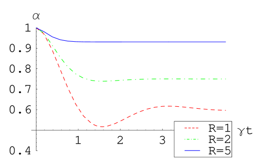
Figure 1: (Color online) Fidelity of the single-qubit code with continuous bit-flip errors and correction, as a function of dimensionless time $\gamma t$, for three different values of the ratio $R=\kappa/\gamma$.

A remarkable difference, however, is that the asymptotic weight outside the code space ($1-\alpha_{*}^{\rm NM}$) decreases with $\kappa$ as $1/\kappa^{2}$, whereas in the Markovian case the same quantity decreases as $1/\kappa$. The asymptotic value can be obtained as an equilibrium point at which the infinitesimal weight flowing out of the code space during a time step $dt$ is equal to the weight flowing into it. The latter corresponds to vanishing right-hand sides in Eqs. (14) and (21). In Sec. IV, we will show that the difference in the equilibrium code-space fidelity for the two different types of decoherence arises from the difference in the corresponding evolutions during initial times.

For multi-qubit codes, error correction cannot preserve a high fidelity with the initial codeword for all times, because there will be multi-qubit errors that can lead to errors within the code space itself. But it is natural to expect that the code-space fidelity can be kept above a certain value, since the effect of the error-correcting map (1) is to oppose its decrease. If similarly to the single-qubit code there is a quadratic difference in the code-space fidelity for the cases of Markovian and non-Markovian decoherence, this could lead to a different performance of the error-correction scheme with respect to the rate of accumulation of uncorrectable errors inside the code space. This is because multi-qubit errors that can lead to transformations entirely within the code space during a time step $dt$ are of order $\textit{O}(dt^{2})$. This means that if the state is kept constantly inside the code space (as in the limit of an infinite error-correction rate), uncorrectable errors will never develop. But if there is a finite nonzero portion of correctable errors, by the error mechanism it will give rise to errors not distinguishable or misinterpreted by the code. Therefore, the weight outside the code space can be thought of as responsible for the accumulation of uncorrectable errors, and consequently a difference in its magnitude may lead to a difference in the overall performance. In the following sections we will see that this is indeed the case.

III The three-qubit bit-flip code

III.1 A Markovian error model

Even though the three-qubit bit-flip code can correct only bit-flip errors, it captures most of the important characteristics of nontrivial stabilizer codes. Before we look at a non-Markovian model, we will review the Markovian case which was studied in PZ98 . Let the system decohere through identical independent bit-flip channels, i.e., $L(\rho)$ is of the form (6) with $\lambda_{1}=\lambda_{2}=\lambda_{3}=\lambda$. Then one can verify that the density matrix at any moment can be written as

$$\rho(t)=a(t)\rho(0)+b(t)\rho_{1}+c(t)\rho_{2}+d(t)\rho_{3},$$ (24)

where

$$\rho_{1}=\frac{1}{3}(X_{1}\rho(0)X_{1}+X_{2}\rho(0)X_{2}+X_{3}\rho(0)X_{3}),$$

$$\rho_{2}=\frac{1}{3}(X_{1}X_{2}\rho(0)X_{1}X_{2}+X_{2}X_{3}\rho(0)X_{2}X_{3}+X_{1}X_{3}\rho(0)X_{1}X_{3}),$$ (25)

$$\rho_{3}=X_{1}X_{2}X_{3}\rho(0)X_{1}X_{2}X_{3},$$

are equally-weighted mixtures of single-qubit, two-qubit and three-qubit errors on the original state.

The effect of decoherence for a single time step $dt$ is equivalent to the following transformation of the coefficients in Eq. (24):

$$\begin{split}a\rightarrow a-3a\lambda dt+b\lambda dt,\\ b\rightarrow b+3a\lambda dt-3b\lambda dt+2c\lambda dt,\\ c\rightarrow c+2b\lambda dt-3c\lambda dt+3d\lambda dt,\\ d\rightarrow d+c\lambda dt-3d\lambda dt.\end{split}$$ (26)

If the system is initially inside the code space, combining Eq. (26) with the effect of the weak error-correcting map $\rho\rightarrow(1-\kappa dt)\rho+\kappa dt\Phi(\rho)$, where $\Phi(\rho)$ is given in Eq. (2), yields the following system of first-order linear differential equations for the evolution of the system subject to decoherence plus error correction:

$$\begin{split}\frac{da(t)}{dt}=-3\lambda a(t)+(\lambda+\kappa)b(t),\\ \frac{db(t)}{dt}=3\lambda a(t)-(3\lambda+\kappa)b(t)+2\lambda c(t),\\ \frac{dc(t)}{dt}=2\lambda b(t)-(3\lambda+\kappa)c(t)+3\lambda d(t),\\ \frac{dd(t)}{dt}=(\lambda+\kappa)c(t)-3\lambda d(t).\end{split}$$ (27)

The exact solution has been found in PZ98 . Here we just note that for the initial conditions $a(0)=1,b(0)=c(0)=d(0)=0$, the exact solution for the weight outside the code space is

$$b(t)+c(t)=\frac{3}{4+r}(1-e^{-(4+r)\lambda t}),$$ (28)

where $r=\kappa/\lambda$. We see that similarly to what we obtained for the trivial code in the previous section, the weight outside the code space quickly decays to its asymptotic value $\frac{3}{4+r}$ which scales as $1/r$. But note that here the asymptotic value is roughly three times greater than that for the single-qubit model. This corresponds to the fact that there are three single-qubit channels. More precisely, it can be verified that if for a given $\kappa$ the uncorrected weight by the single-qubit scheme is small, then the uncorrected weight by a multi-qubit code using the same $\kappa$ and the same kind of decoherence for each qubit scales approximately linearly with the number of qubits OBinprep . Similarly, the ratio $r$ required to preserve a given overlap with the code space scales linearly with the number of qubits in the code.

The most important difference from the single-qubit model is that in this model there are uncorrectable errors that cause a decay of the state’s fidelity inside the code space. Due to the finiteness of the resources employed by our scheme, there always remains a nonzero portion of the state outside the code space, which gives rise to uncorrectable three-qubit errors. To understand how the state decays inside the code space, we ignore the terms of the order of the weight outside the code space in the exact solution. We obtain:

$$a(t)\approx\frac{1+e^{-\frac{6}{r}2\lambda t}}{2}\approx 1-d(t),$$ (29)

$$b(t)\approx c(t)\approx 0.$$ (30)

Comparing this solution to the expression for the fidelity of a single decaying qubit without error correction—which can be seen from Eq. (15) for $\kappa=0$—we see that the encoded qubit decays roughly as if subject to bit-flip decoherence with rate $6\lambda/r$. Therefore, for large $r$ this error-correction scheme can reduce the rate of decoherence approximately $r/6$ times. In the limit $r\rightarrow\infty$, it leads to perfect protection of the state for all times.

III.2 A non-Markovian error model

We consider a model where each qubit independently undergoes the same kind of non-Markovian decoherence as the one we studied for the single-qubit code. Here the system we look at consists of six qubits - three for the codeword and three for the environment. We assume that all system qubits are coupled to their corresponding environment qubits with the same coupling strength, i.e., the Hamiltonian is

$$H=\gamma\overset{3}{\underset{i=1}{\sum}}X^{S}_{i}\otimes X^{B}_{i},$$ (31)

where the operators $X^{S}$ act on the system qubits and $X^{B}$ act on the corresponding bath qubits. The subscripts label the particular qubit on which they act. Obviously, the types of effective single-qubit errors on the density matrix of the system that can result from this Hamiltonian at any time, whether they are CP or not, will have operator elements which are linear combinations of $I$ and $X^{S}$, i.e., they are correctable by the procedure according to ShaLid06 . Considering the forms of the Hamiltonian (31) and the error-correcting map (2), one can see that the density matrix of the entire system at any moment is a linear combination of terms of the following type:

$$\varrho_{lmn,pqr}\equiv X_{1}^{l}X_{2}^{m}X_{3}^{n}\rho(0)X_{1}^{p}X_{2}^{q}X_{3}^{r}\otimes\frac{X_{1}^{l+p}}{2}\otimes\frac{X_{2}^{m+q}}{2}\otimes\frac{X_{3}^{n+r}}{2}.$$ (32)

Here the first term in the tensor product refers to the Hilbert space of the system, and the following three refer to the Hilbert spaces of the bath qubits that couple to the first, second and third qubits from the code, respectively. The powers $l,m,n,p,q,r$ take values $0$ and $1$ in all possible combinations, and $X^{1}=X$, $X^{0}=X^{2}=I$. Note that $\varrho_{lmn,pqr}$ should not be mistaken for the components of the density matrix in the computational basis. Collecting these together, we can write the density matrix in the form

$$\rho(t) = \underset{l,m,n,p,q,r}{\sum}(-i)^{l+m+n}(i)^{p+q+r}C_{lmn,pqr}(t)\times\varrho_{lmn,pqr},$$ (33)

where the coefficients $C_{lmn,pqr}(t)$ are real. The coefficient $C_{000,000}$ is less than or equal to the codeword fidelity (with equality when $\rho(0)=|\bar{0}\rangle\langle\bar{0}|$ or $\rho(0)=|\bar{1}\rangle\langle\bar{1}|$). Since the scheme is intended to protect an unknown codeword, we are interested in its worst-case performance; we will therefore use $C_{000,000}$ as a lower bound on the codeword fidelity.

Using the symmetry with respect to permutations of the different system-bath pairs of qubits and the Hermiticity of the density matrix, we can reduce the description of the evolution to a system of equations for only $13$ of the $64$ coefficients. (In fact, $12$ coefficients are sufficient if we invoke the normalization condition $\textrm{Tr}\rho=1$, but we have found it more convenient to work with $13$.) The equations are linear, and we write them as a single 13-dimensional vector equation:

$$\frac{d}{dt}\begin{bmatrix}C_{000,000}\\ C_{100,000}\\ C_{110,000}\\ C_{100,010}\\ C_{100,100}\\ C_{110,001}\\ C_{111,000}\\ C_{110,100}\\ C_{110,110}\\ C_{110,011}\\ C_{111,100}\\ C_{111,110}\\ C_{111,111}\end{bmatrix}=\gamma\setcounter{MaxMatrixCols}{13}\begin{bmatrix}0&-6&0&0&3R&0&0&0&0&0&0&0&0\\ 1&-R&-2&-2&-1&0&0&0&0&0&0&0&0\\ 0&2&-R&0&0&-1&-1&-2&0&0&0&0&0\\ 0&2&0&-R&0&-2&0&-2&0&0&0&0&0\\ 0&2&0&0&-R&0&0&-4&0&0&0&0&0\\ 0&0&1&2&0&-R&0&0&0&-2&-1&0&0\\ 0&0&3&0&0&-3R&0&0&0&0&-3&0&0\\ 0&0&1&1&1&0&0&-R&-1&-1&-1&0&0\\ 0&0&0&0&0&0&0&4&-R&0&0&-2&0\\ 0&0&0&0&0&2&0&2&0&-R&0&-2&0\\ 0&0&0&0&0&1&1&2&0&0&-R&-2&0\\ 0&0&0&0&0&0&0&0&1&2&2&-R&-1\\ 0&0&0&0&0&0&0&0&3R&0&0&6&0\end{bmatrix}\cdot\begin{bmatrix}C_{000,000}\\ C_{100,000}\\ C_{110,000}\\ C_{100,010}\\ C_{100,100}\\ C_{110,001}\\ C_{111,000}\\ C_{110,100}\\ C_{110,110}\\ C_{110,011}\\ C_{111,100}\\ C_{111,110}\\ C_{111,111}\end{bmatrix}$$ (34)

where $R=\kappa/\gamma$. Each nonzero component in this matrix represents an allowed transition process for the quantum states; these transitions can be driven either by the decoherence process or the continuous error-correction process. We plot these allowed transitions in Fig. 2.

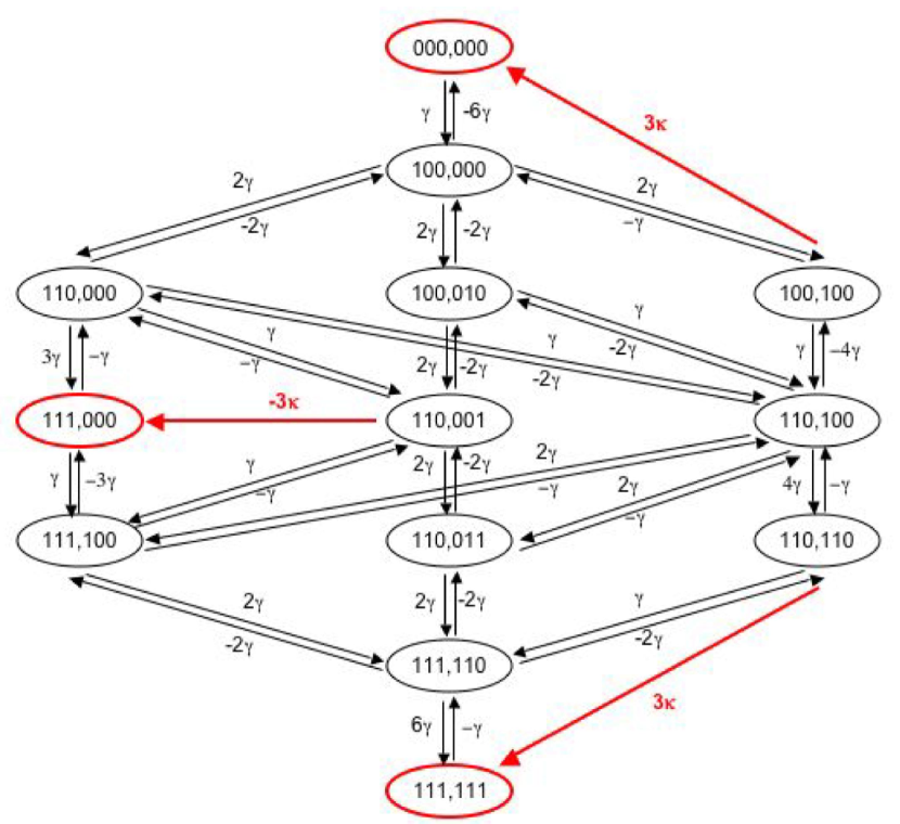
Figure 2: (Color online) These are the allowed transitions between the different components of the system (34) and their rates, arising from both the decoherence (bit-flip) process (with rate $\gamma$ and the continuous error-correction process (with rate $\kappa$). Online, the transitions due to decoherence are black, and the transitions due to error correction are red.

We can use the symmetries of the process to recover the 64 coefficients of the full state. Each of the 13 coefficients represents a set of coefficients having the same number of $1$s on the left and the same number of $1$s on the right, as well as the same number of places which have $1$ on both sides. All such coefficients are equal at all times. For example, the coefficient $C_{110,011}$ is equal to all coefficients with two $1$s on the left, two $1$s on the right and exactly one place with $1$ on both sides; there are exactly six such coefficients:

$$C_{110,011}=C_{110,101}=C_{101,011}=C_{101,110}=C_{011,110}=C_{011,101}.$$

In determining the transfer rate from one coefficient to another in Fig. 2, one has to take into account the number of different coefficients of the first type which can make a transition to a coefficient of the second type of order $dt$ according to Eq. (11). The sign of the flow is determined from the phases in front of the coefficients in Eq. (33).

The eigenvalues of the matrix in Eq. (34) up to the first two lowest orders in $1/\kappa$ are presented in Table I.

Table 1: Eigenvalues of the matrix

Eigenvalues
$\lambda_{0}=0$
$\lambda_{1,2}=-\kappa$
$\lambda_{3,4}=-\kappa\pm i2\gamma$
$\lambda_{5,6}=-\kappa\pm i4\gamma$
$\lambda_{7,8}=-\kappa\pm i(\sqrt{13}+3)\gamma+\textit{O}(1/\kappa)$
$\lambda_{9,10}=-\kappa\pm i(\sqrt{13}-3)\gamma+\textit{O}(1/\kappa)$
$\lambda_{11,12}=\pm i(24/R^{2})\gamma-(144/R^{3})\gamma+\textit{O}(1/\kappa^{4})$

Obviously all eigenvalues except the first one and the last two describe fast decays with rates $\sim\kappa$. They correspond to terms in the solution which will vanish quickly after the beginning of the evolution. The eigenvalue $0$ corresponds to the asymptotic ($t\rightarrow\infty$) solution, since all other terms will eventually decay. The last two eigenvalues are those that play the main role in the evolution on a time scale $t\gg\frac{1}{\kappa}$. We see that on such a time scale, the solution will contain an oscillation with an angular frequency approximately equal to $(24/R^{2})\gamma$ which is damped by a decay factor with a rate of approximately $(144/R^{3})\gamma$. In Fig. 3 we have plotted the codeword fidelity $C_{000,000}(t)$ as a function of the dimensionless parameter $\gamma t$ for $R=100$. The graph indeed represents this type of behavior, except for very short times after the beginning ($\gamma t\sim 0.1$), where one can see a fast but small in magnitude decay (Fig. 4). The maximum magnitude of this quickly decaying term obviously decreases with $R$, since in the limit of $R\rightarrow\infty$ the fidelity should remain constantly equal to $1$.

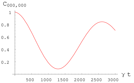
Figure 3: (Color online) Long-time behavior of three-qubit system with bit-flip noise and continuous error correction. The ratio of correction rate to decoherence rate is $R=\kappa/\gamma=100$.

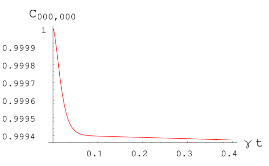
Figure 4: (Color online) Short-time behavior of three-qubit system with bit-flip noise and continuous error correction. The ratio of correction rate to decoherence rate is $R=\kappa/\gamma=100$.

From the form of the eigenvalues one can see that as $R$ increases, the frequency of the main oscillation decreases as $1/R^{2}$ while the rate of decay decreases faster, as $1/R^{3}$. Thus in the limit $R\rightarrow\infty$, the evolution approaches an oscillation with an angular frequency $(24/R^{2})\gamma$. (We formulate this statement more rigorously below.) This is the same type of evolution as that of a single qubit interacting with its environment, but the coupling constant is effectively reduced by a factor of $R^{2}/12$.

While the coupling constant serves to characterize the decoherence process in this particular case, this is not valid in general. To handle the more general situation, we propose to use the instantaneous rate of decrease of the codeword fidelity $F_{cw}$ as a measure of the effect of decoherence:

$$\Lambda(F_{cw}(t))=-\frac{dF_{cw}(t)}{dt}.$$ (35)

(In the present case, $F_{cw}=C_{000,000}$.) This quantity does not coincide with the decoherence rate in the Markovian case (which can be defined naturally from the Lindblad equation), but it is a good estimate of the rate of loss of fidelity and can be used for any decoherence model. From now on we will refer to it simply as an error rate, but we note that there are other possible definitions of instantaneous error rate suitable for non-Markovian decoherence, which in general may depend on the kind of errors they describe. Since the goal of error correction is to preserve the codeword fidelity, the quantity (35) is a useful indicator for the performance of a given scheme. Note that $\Lambda(F_{cw})$ is a function of the codeword fidelity and therefore it makes sense to use it for a comparison between different cases only for identical values of $F_{cw}$. For our example, the fact that the coupling constant is effectively reduced approximately $R^{2}/12$ times implies that the error rate for a given value of $F_{cw}$ is also reduced $R^{2}/12$ times. Similarly, the reduction of $\lambda$ by the factor $r/6$ in the Markovian case implies a reduction of $\Lambda$ by the same factor. We see that the effective reduction of the error rate increases quadratically with $\kappa^{2}$ in the non-Markovian case, whereas it increases only linearly with $\kappa$ in the Markovian case.

Now let us rigorously derive the approximate solution to this model of non-Markovian decoherence with continuous error correction. Assuming that $\gamma\ll\kappa$ (or equivalently, $R\gg 1$), the superoperator driving the evolution of the system during a time step $\delta t$ can be written as

$$e^{\mathcal{L}\delta t} = e^{\mathcal{L}_{\kappa}\delta t}+\overset{\delta t}{\underset{0}{\int}}dt^{\prime}e^{\mathcal{L}_{\kappa}(\delta t-t^{\prime})}\mathcal{L}_{\gamma}e^{\mathcal{L}_{\kappa}t^{\prime}}+\overset{\delta t}{\underset{0}{\int}}dt^{\prime}\overset{\delta t}{\underset{t^{\prime}}{\int}}dt^{\prime\prime}e^{\mathcal{L}_{\kappa}(\delta t-t^{\prime\prime})}\mathcal{L}_{\gamma}e^{\mathcal{L}_{\kappa}(t^{\prime\prime}-t^{\prime})}\mathcal{L}_{\gamma}e^{\mathcal{L}_{\kappa}t^{\prime}}+$$ (36)

$$+ \overset{\delta t}{\underset{0}{\int}}dt^{\prime}\overset{\delta t}{\underset{t^{\prime}}{\int}}dt^{\prime\prime}\overset{\delta t}{\underset{t^{\prime\prime}}{\int}}dt^{\prime\prime\prime}e^{\mathcal{L}_{\kappa}(\delta t-t^{\prime\prime\prime})}\mathcal{L}_{\gamma}e^{\mathcal{L}_{\kappa}(t^{\prime\prime\prime}-t^{\prime\prime})}\mathcal{L}_{\gamma}e^{\mathcal{L}_{\kappa}(t^{\prime\prime}-t^{\prime})}\mathcal{L}_{\gamma}e^{\mathcal{L}_{\kappa}t^{\prime}}+...$$

We have denoted the Liouvillian by $\mathcal{L}=\mathcal{L}_{\gamma}+\mathcal{L}_{\kappa}$, where $\mathcal{L}_{\kappa}\rho=\kappa\Gamma(\rho)$, and $\mathcal{L}_{\gamma}\rho=-i[H,\rho]$.

Let $\gamma\delta t\ll 1\ll\kappa\delta t$. We will derive an approximate differential equation for the evolution of $\rho(t)$ by looking at the terms of order $\delta t$ in the change of $\rho$ according to Eq. (36). When $\kappa=0$, we have $d\rho/dt=\mathcal{L}_{\gamma}\rho$, so the effect of $\mathcal{L}_{\gamma}$ on the state of the system can be seen from Eq. (34) with $\kappa$ taken equal to $0$. By the action of $\exp({\mathcal{L}_{\kappa}t})$, the different terms of the density matrix transform as follows: $\varrho_{000,000},\varrho_{111,000},\varrho_{111,111}$ remain unchanged, $\varrho_{100,100}\rightarrow e^{-\kappa t}\varrho_{100,100}+(1-e^{-\kappa t})\varrho_{000,000}$, $\varrho_{110,110}\rightarrow e^{-\kappa t}\varrho_{110,110}+(1-e^{-\kappa t})\varrho_{111,111}$, $\varrho_{110,001}\rightarrow e^{-\kappa t}\varrho_{110,001}-(1-e^{-\kappa t})\varrho_{111,000}$, and all other terms are changed as $\varrho\rightarrow e^{-\kappa t}\varrho$. Since $\kappa\delta t\gg 1$, we will ignore terms of order $e^{-\kappa\delta t}$. But from Eq. (36) it can be seen that all terms except $\varrho_{000,000},\varrho_{111,000},\varrho_{000,111},\varrho_{111,111}$ will get multiplied by the factor $e^{-\kappa\delta t}$ by the action of $\exp({\mathcal{L}_{\kappa}\delta t})$ in Eq. (36). The integrals in Eq. (36) also yield negligible factors, since every integral either gives rise to a factor of order $\delta t$ when the integration variable is trivially integrated, or a factor of $1/\kappa$ when the variable participates nontrivially in the exponent. Therefore, in the above approximation these terms of the density matrix can be neglected, which amounts to an effective evolution entirely within the code space. According to Eq. (34), the terms $\varrho_{000,000},\varrho_{111,000},\varrho_{111,111}$ can couple to each other only by a triple or higher application of $\mathcal{L}_{\gamma}$. This means that if we consider the expansion up to the lowest nontrivial order in $\gamma$, we only need to look at the triple integral in Eq. (36).

Let us consider the effect of $\exp({\mathcal{L}\delta t})$ on $C_{000,000}$. Any change can come directly only from $\varrho_{111,000}$ and $\varrho_{000,111}$. The first exponent $e^{\mathcal{L}_{\kappa}t^{\prime}}$ acts on these terms as the identity. Under the action of the first operator $\mathcal{L}_{\gamma}$ each of these two terms can transform to six terms that can eventually be transformed to $\varrho_{000,000}$. They are $\varrho_{110,000}$, $\varrho_{101,000}$, $\varrho_{011,000}$, $\varrho_{111,100}$, $\varrho_{111,010}$, $\varrho_{111,001}$, and $\varrho_{000,110}$, $\varrho_{000,101}$, $\varrho_{000,011}$, $\varrho_{100,111}$, $\varrho_{010,111}$, $\varrho_{001,111}$, with appropriate factors. The action of the second exponent is to multiply each of these new terms by $e^{-\kappa(t^{\prime\prime}-t^{\prime})}$. After the action of the second $\mathcal{L}_{\gamma}$, the action of the third exponent on the relevant resultant terms will be again to multiply them by a factor $e^{-\kappa(t^{\prime\prime\prime}-t^{\prime\prime})}$. Thus the second and the third exponents yield a net factor of $e^{-\kappa(t^{\prime\prime\prime}-t^{\prime})}$. After the second and the third $\mathcal{L}_{\gamma}$, the relevant terms that we get are $\varrho_{000,000}$ and $\varrho_{100,100}$, $\varrho_{010,010}$, $\varrho_{001,001}$, each with a corresponding factor. Finally, the last exponent acts as the identity on $\varrho_{000,000}$ and transforms each of the terms $\varrho_{100,100}$, $\varrho_{010,010}$, $\varrho_{001,001}$ into $(1-e^{-\kappa(\delta t-t^{\prime\prime\prime})})\varrho_{000,000}$. Counting the number of different terms that arise at each step, and taking into account the factors that accompany them, we obtain:

$$C_{000,000} \rightarrow C_{000,000}+\overset{\delta t}{\underset{0}{\int}}dt^{\prime}\overset{\delta t}{\underset{t^{\prime}}{\int}}dt^{\prime\prime}\overset{\delta t}{\underset{t^{\prime\prime}}{\int}}dt^{\prime\prime\prime}(24e^{-\kappa(t^{\prime\prime\prime}-t^{\prime})}-36e^{-\kappa(\delta t-t^{\prime})})C_{111,000}+\cdots$$ (37)

$$\approx C_{000,000}+C_{111,000}\frac{24}{R^{2}}\gamma\delta t+\textit{O}(\delta t^{2}).$$

Using that $C_{000,000}+C_{111,111}\approx 1$, in a similar way one obtains

$$C_{111,000}\rightarrow C_{111,000}-(2C_{000,000}-1)\frac{12}{R^{2}}\gamma\delta t+\textit{O}(\delta t^{2}).$$ (38)

For times much larger than $\delta t$, we can write the approximate differential equations

$$\frac{dC_{000,000}}{dt}=\frac{24}{R^{2}}\gamma C_{111,000},$$

$$\frac{dC_{111,000}}{dt}=-\frac{12}{R^{2}}\gamma(2C_{000,000}-1).$$ (39)

Comparing with Eq. (19), we see that the encoded qubit undergoes approximately the same type of evolution as that of a single qubit without error correction, but the coupling constant is effectively decreased $R^{2}/12$ times. The solution of Eq. (39) yields for the codeword fidelity

$$C_{000,000}(t)=\frac{1+\cos(\frac{24}{R^{2}}\gamma t)}{2}.$$ (40)

This solution is valid only with precision $\textit{O}(1/R)$ for times $\gamma t\ll R^{3}$. This is because we ignored terms whose magnitudes are always of order $\textit{O}(1/R)$ and ignored changes of order $\textit{O}(\gamma\delta t/R^{3})$ per time step $\delta t$ in the other terms. The latter changes could accumulate with time and become of the order of unity for times $\gamma t\approx R^{3}$, which is why the approximate solution is invalid for such times. In fact, if one carries out the expansion (36) to fourth order in $\gamma$, one obtains the approximate equations

$$\frac{dC_{000,000}}{dt}=\frac{24}{R^{2}}\gamma C_{111,000}-\frac{72}{R^{3}}\gamma(2C_{000,000}-1),$$

$$\frac{dC_{111,000}}{dt}=-\frac{12}{R^{2}}\gamma(2C_{000,000}-1)-\frac{144}{R^{3}}\gamma C_{111,000},$$ (41)

which yield for the fidelity

$$C_{000,000}(t)=\frac{1+e^{-144\gamma t/R^{3}}\cos(24\gamma t/R^{2})}{2}.$$ (42)

We see that in addition to the effective error process which is of the same type as that of a single qubit, there is an extra Markovian bit-flip process with rate $72\gamma/R^{3}$. This Markovian behavior is due to the Markovian character of our error-correcting procedure which, at this level of approximation, is responsible for the direct transfer of weight between $\varrho_{000,000}$ and $\varrho_{111,111}$, and between $\varrho_{111,000}$ and $\varrho_{000,111}$. The exponential factor explicitly reveals the range of applicability of solution (40): with precision $\textit{O}(1/R)$, it is valid only for times $\gamma t$ of up to order $R^{2}$. For times of the order of $R^{3}$, the decay becomes significant and cannot be neglected. The exponential factor may also play an important role for short times of up to order $R$, where its contribution is bigger than that of the cosine. But in the latter regime the difference between the cosine and the exponent is of order $\textit{O}(1/R^{2})$, which is negligible for the precision that we consider.

In general, the effective evolution that one obtains in the limit of high error-correction rate does not have to approach a form identical to that of a single decohering qubit. The reason we obtain such behavior here is that for this particular model the lowest order of uncorrectable errors that transform the state within the code space is 3, and three-qubit errors have the form of an encoded $X$ operation. Furthermore, the symmetry of the problem ensured an identical evolution of the three qubits in the code. For general stabilizer codes, the errors that a single qubit can undergo are not limited to bit flips only. Therefore, different combinations of single-qubit errors may lead to different types of lowest-order uncorrectable errors inside the code space, none of which in principle has to represent an encoded version of the single-qubit operations that compose it. In addition, if the noise is different for the different qubits, there is no unique single-qubit error model to compare to. Nevertheless, we will show that with regard to the effective decrease in the error-correction rate, general stabilizer codes will exhibit the same qualitative performance.

IV Relation to the Zeno regime

The effective continuous evolution (39) was derived under the assumption that $\gamma\delta t\ll 1\ll\kappa\delta t$. The first inequality implies that $\delta t$ can be considered within the Zeno time scale of the system’s evolution without error correction. On the other hand, from the relation between $\kappa$ and $\tau_{c}$ in (4) we see that $\tau_{c}\ll\delta t$. Therefore, the time for implementing a weak error-correcting operation has to be sufficiently small so that on the Zeno time scale the error-correction procedure can be described approximately as a continuous Markovian process. This suggests a way of understanding the quadratic enhancement in the non-Markovian case based on the properties of the Zeno regime.

Let us consider again the single-qubit code from Sec. II, but this time let the error model be any Hamiltonian-driven process. We assume that the qubit is initially in the state $|0\rangle$, i.e., the state of the system including the bath has the form $\rho(0)=|0\rangle\langle 0|\otimes\rho_{B}(0)$. For times smaller than the Zeno time $\delta t_{Z}$, the evolution of the fidelity without error correction can be described by Eq. (9). Equation (9) naturally defines the Zeno regime in terms of $\alpha$ itself:

$$\alpha\geq\alpha_{Z}\equiv 1-C\delta t_{Z}^{2}.$$ (43)

For a single time step $\Delta t\ll\delta t_{Z}$, the change in the fidelity is

$$\alpha\rightarrow\alpha-2\sqrt{C}\sqrt{1-\alpha}\Delta t+\textit{O}(\Delta t^{2}).$$ (44)

On the other hand, the effect of error correction during a time step $\Delta t$ is

$$\alpha\rightarrow\alpha+\kappa(1-\alpha)\Delta t+\textit{O}(\Delta t^{2}),$$ (45)

i.e., it tends to oppose the effect of decoherence. If both processes happen simultaneously, the effect of decoherence will still be of the form (44), but the coefficient $C$ may vary with time. This is because the presence of error-correction opposes the decrease of the fidelity and consequently can lead to an increase in the time for which the fidelity remains within the Zeno range. If this time is sufficiently long, the state of the environment could change significantly under the action of the Hamiltonian, thus giving rise to a different value for $C$ in Eq. (44) according to Eq. (10).

Note that the strength of the Hamiltonian puts a limit on $C$, and therefore this constant can vary only within a certain range. The equilibrium fidelity $\alpha_{*}^{\rm NM}$ that we obtained for the error model in Sec. II, can be thought of as the point at which the effects of error and error correction cancel out. For a general model, where the coefficient $C$ may vary with time, this leads to a quasi-stationary equilibrium. From Eqs. (44) and (45), one obtains the equilibrium fidelity

$$\alpha_{*}^{\rm NM}\approx 1-\frac{4C}{\kappa^{2}}.$$ (46)

In agreement with what we obtained in Sec. II, the equilibrium fidelity differs from $1$ by a quantity proportional to $1/\kappa^{2}$. This quantity is generally quasi-stationary and can vary within a limited range. If one assumes a Markovian error model, for short times the fidelity changes linearly with time which leads to $1-\alpha_{*}^{\rm M}\propto 1/\kappa$. Thus the difference can be attributed to the existence of a Zeno regime in the non-Markovian case.

But what happens in the case of non-trivial codes? As we saw, there the state decays inside the code space and therefore can be highly correlated with the environment. Can we talk about a Zeno regime then? It turns out that the answer is positive. Assuming that each qubit undergoes an independent error process, then up to first order in $\Delta t$ the Hamiltonian cannot map terms in the code space to other terms without detectable errors. (This includes both terms in the code space and terms from the hidden part, like $\varrho_{111,000}$ in the example of the bit-flip code.) It can only transform terms from the code space into traceless terms from the hidden part which correspond to single-qubit errors (like $\varrho_{100,000}$ in the same example). Let $|\bar{0}\rangle$, $|\bar{1}\rangle$ be the two logical codewords and $|\psi_{i}\rangle$ be an orthonormal basis that spans the space of all single-qubit errors. Then in the basis $|\bar{0}\rangle$, $|\bar{1}\rangle$, $|\psi_{i}\rangle$, all the terms that can be coupled directly to terms inside the code space are $|\bar{0}\rangle\langle\psi_{i}|$, $|\psi_{i}\rangle\langle\bar{0}|$, $|\bar{1}\rangle\langle\psi_{i}|$, $|\psi_{i}\rangle\langle\bar{1}|$. From the condition of positivity of the density matrix, one can show that the coefficients in front of these terms are at most $\sqrt{\alpha(1-\alpha)}$ in magnitude, where $\alpha$ is the code-space fidelity. This implies that for small enough $1-\alpha$, the change in the code-space fidelity is of the type (44), which is Zeno-like behavior. Then using only the properties of the Zeno behavior as we did above, we can conclude that the weight outside the code space will be kept at a quasi-stationary value of order $1/\kappa^{2}$. Since uncorrectable errors enter the code space through the action of the error-correction procedure, which misinterprets some multi-qubit errors in the error space, the effective error rate will be limited by a factor proportional to the weight in the error space. That is, this will lead to an effective decrease of the error rate at least by a factor proportional to $1/\kappa^{2}$.

The accumulation of uncorrectable errors in the Markovian case is similar, except that in this case there is a direct transfer of errors between the code space and the visible part of the error space. In both cases, the error rate is effectively reduced by a factor which is roughly proportional to the inverse of the weight in the error space, and therefore the difference in the performance comes from the difference in this weight. The quasi-stationary equilibrium value of the code-space fidelity establishes a quasi-stationary flow between the code space and the error space. One can think that this flow effectively takes non-erroneous weight from the code space, transports it through the error space where it accumulates uncorrectable errors, and brings it back into the code space. Thus by minimizing the weight outside the code space, error correction creates a “bottleneck” which reduces the rate at which uncorrectable errors accumulate.

Finally, a brief remark about the resources needed for quadratic reduction of the error rate. As pointed out above, two conditions are involved: one concerns the rate of error correction; the other concerns the time resolution of the weak error-correcting operations. Both of these quantities must be sufficiently large. There is, however, an interplay between the two, which involves the strength of the interaction required to implement the weak error-correcting map (3). Let us imagine that the weak map is implemented by making the system interact weakly with an ancilla in a given state, after which the ancilla is discarded. The error-correction procedure consists of a sequence of such interactions, and can be thought of as a cooling process which takes away the entropy accumulated in the system as a result of correctable errors. If the time for which a single ancilla interacts with the system is $\tau_{c}$, one can verify that the parameter $\varepsilon$ in Eq. (3) would be proportional to $g^{2}\tau_{c}^{2}$, where $g$ is the coupling strength between the system and the ancilla. From Eq. (4) we then obtain that

$$\kappa\propto g^{2}\tau_{c}.$$ (47)

The two parameters that can be controlled are the interaction time and the interaction strength, and they determine the error-correction rate. Thus if $g$ is kept constant, a decrease in the interaction time $\tau_{c}$ leads to a proportional decrease in $\kappa$, which may be undesirable. In order to achieve a good working regime, one may need to adjust both $\tau_{c}$ and $g$. But it has to be pointed out that in some situations decreasing $\tau_{c}$ alone can prove advantageous, if it leads to a time resolution revealing the non-Markovian character of an error model which was previously described as Markovian. The quadratic enhancement of the performance as a function of $\kappa$ may compensate the decrease in $\kappa$, thus leading to a seemingly paradoxical result: better performance with a lower error-correction rate.

V Conclusion

In this paper we studied the performance of a particular continuous quantum error-correction scheme for non-Markovian errors. We analyzed the evolution of the single-qubit code and the three-qubit bit-flip code in the presence of continuous error correction for a simple non-Markovian bit-flip error model. This enabled us to understand the workings of the error-correction scheme, and the mechanism whereby uncorrectable errors accumulate. The fidelity of the state with the code space in both examples quickly reaches an equilibrium value, which can be made arbitrarily close to $1$ by a sufficiently high rate of error correction. The weight of the density matrix outside the code space scales as $1/\kappa$ in the Markovian case, while it scales as $1/\kappa^{2}$ in the non-Markovian case. Correspondingly, the rate at which uncorrectable errors accumulate in the three-qubit code is proportional to $1/\kappa$ in the Markovian case, and to $1/\kappa^{2}$ in the non-Markovian case. These differences have the same cause, since the equilibrium weight in the error space is closely related to the rate of uncorrectable error accumulation.

The quadratic difference in the error weight between the Markovian and non-Markovian cases can be attributed to the existence of a Zeno regime in the non-Markovian case. Regardless of the correlations between the density matrix inside the code space and the environment, if the lowest-order errors are correctable by the code, there exists a Zeno regime in the evolution of the code-space fidelity. The effective reduction of the error rate with the rate of error correction for non-Markovian error models depends crucially on the assumption that the time resolution of the continuous error correction is much shorter than the Zeno time scale of the evolution without error correction. This suggests that decreasing the time for a single (infinitesimal) error-correcting operation can lead to an increase in the performance of the scheme, even if the average error-correction rate goes down.

While in this paper we have only considered codes for the correction of single-qubit errors, our results can be extended to other types of codes and errors as well. As long as the error process only produces errors correctable by the code to lowest order, an argument analogous to the one given here shows that a Zeno regime will exist, which leads to an enhancement in the error-correction performance. Unfortunately, it is very difficult to describe the evolution of a system with a continuous correction protocol, based on a general error-correction code and subject to general non-Markovian interactions with the environment. This is especially true if one must include the evolution of a complicated environment in the description, as would be necessary in general. A more practical step in this direction might be to find an effective description for the evolution of the reduced density matrix of the system subject to decoherence plus error correction, using projection techniques like the Nakajima-Zwanzig or the TCL master equations. Since one is usually interested in the evolution during initial times before the codeword fidelity decreases significantly, a perturbation approach could be useful. This is a subject for further research.

References

- (1) P. Shor, in Proceedings of the Annual Symposium on Fundamentals of Computer Science, 56-65, IEEE Press, Los Alamitos, CA (1996).
- (2) D. Aharonov and M. Ben-Or, in Proceedings of the Annual ACM Symposium on Theory of Computing, 176, ACM, New York (1998).
- (3) A. Kitaev, Russian Math. Surveys 52, 1191 (1997).
- (4) E. Knill, R. Laflamme, and W. H. Zurek, Proc. R. Soc. London, Ser. A 454, 365 (1998).
- (5) D. Gottesman, Stabilizer codes and quantum error orrection, Ph.D. thesis, Caltech, 1997, quant-ph/9705052.
- (6) P. Shor, Phys. Rev. A 52, 2493 (1995).
- (7) A. M. Steane, Phys. Rev. Lett. 77, 793 (1996).
- (8) E. Knill, R. Laflamme, quant-ph/9608012.
- (9) J. P. Paz and W. H. Zurek, Proc. R. Soc. London, Ser. A 454, 355 (1998).
- (10) M. Sarovar and G. J. Milburn, Phys. Rev. A. 72 012306 (2005).
- (11) O. Oreshkov and T. A. Brun, in preparation.
- (12) C. Ahn, A. C. Doherty, and A. J. Landahl, Phys. Rev. A 65, 042301 (2002).
- (13) M. Sarovar and G. J. Milburn, Quantum Communication, Measurement Computing, (AIP Conference Proceeedings), p.121 (2004).
- (14) H.-P. Breuer and F. Petruccione, The Theory of Open Quantum Systems (Oxford University Press, Oxford, 2002).
- (15) G. Lindblad, Commun. Math. Phys. 48, 119 (1976).
- (16) B. Misra and E.C.G Sudarshan, J. Math. Phys. 18, 756 (1977).
- (17) H. Nakazato, M. Namiki, and S. Pascazio, Int. J. Mod. Phys. B 10, 247 (1996).
- (18) W. H. Zurek, Phys. Rev. Lett. 53, 391 (1984).
- (19) A. Barenco, A. Berthiaume, D. Deutsch, A. Eckert, R. Jozsa, and C. Macchiavello, SIAM Journal on Computing 26, 1541 (1997).
- (20) L. Vaidman, L. Goldenberg, and S. Wiesner, Phys. Rev. A, 54, 1745 (1996).
- (21) T. Quang, M. Woldeyohannes, S. John, and G. S. Agraval, Phys. Rev. Lett. 79, 5238 (1997).
- (22) H.-P. Breuer, D. Burgarth, and F. Petruccione, Phys. Rev. B 70, 045323 (2004).
- (23) H. Krovi, O. Oreshkov, M Ryazonov, and D. Lidar, arXiv:0707.2096.
- (24) A. Shabani and D. Lidar, quant-ph/0610028.
- (25) B. M. Terhal and G. Burkard, Phys. Rev. A 71, 012336 (2005).
- (26) P. Aliferis, D. Gottesman, and J. Preskill, Quantum Inf. Comput. 6, 97 (2006).
- (27) D. Aharonov, A. Kitaev, and J. Preskill, Phys. Rev. Lett. 96, 050504 (2006).
- (28) S. Nakajima, Prog. Theor. Phys. 20, 948 (1958).
- (29) R. Zwanzig, J. Chem. Phys. 33, 1338 (1960).
- (30) F. Shibata, Y. Takahashi, and N. Hashitsume, J. Stat. Phys. 17, 171 (1977).
- (31) F. Shibata and T. Arimitsu, J. Phys. Soc. Jpn. 49, 891 (1980).