Localization and chiral symmetry in 2+1 flavor domain wall QCD

Abstract

We present results for the dependence of the residual mass of domain wall fermions (DWF) on the size of the fifth dimension and its relation to the density and localization properties of low-lying eigenvectors of the corresponding hermitian Wilson Dirac operator relevant to simulations of 2+1 flavor domain wall QCD. Using the DBW2 and Iwasaki gauge actions, we generate ensembles of configurations with a $16^{3}\times 32$ space-time volume and an extent of 8 in the fifth dimension for the sea quarks. We demonstrate the existence of a regime where the degree of locality, the size of chiral symmetry breaking and the rate of topology change can be acceptable for inverse lattice spacings $a^{-1}\geq 1.6$ GeV.

I Introduction

In this paper we present a study of three closely related quantities that are important for the successful application of the domain wall fermion (DWF) formulation to full QCD calculations with 2+1 flavors of light quarks. The first of these is the size of the explicit chiral symmetry breaking that occurs for domain wall fermions due to the finite extent of the lattice in the fifth dimension. This is usually characterized by the residual mass, $m_{\rm res}$, whose dependence on the gauge action, gauge coupling and the extent of the fifth dimension is discussed.

The second topic covers the spectral properties of the four-dimensional hermitian Wilson Dirac operator evaluated at large, negative mass, $-M_{5}$. All current formulations of lattice chiral symmetry make use of a negative–mass (hermitian) Wilson Dirac operator, $H_{W}=\gamma_{5}D_{W}$, and intellectually derive from the Kaplan approach Kaplan (1992), whether by taking an analytic limit as in the overlap operator Neuberger (1998a), or by directly simulating a finite fifth dimension Furman and Shamir (1995) of size $L_{s}$. Auxiliary information on the nature of the spectrum of $H_{W}$ is required to have confidence that a simulation at fixed lattice spacing lies in the universality class of QCD. This topic is closely connected to the properties of the Aoki phase of the related operator $D_{W}$ Aoki (1984). If a chiral fermion calculation is attempted for a gauge action and a negative fermion mass that is too close to the Aoki phase, undesirable non-locality or enhanced explicit chiral symmetry breaking may result. Thus, we will examine both the density of the low-lying eigenmodes of $H_{W}$ and their locality properties.

Finally, we examine the ergodicity of the sampling of topological charge that results for these choices of gauge action and negative Wilson Dirac mass using the rational hybrid Monte Carlo method of Clark and Kennedy Clark and Kennedy (2004); Clark et al. (2005). Since a change in the topological charge of an evolving lattice configuration is expected to be accompanied by a zero mode of $H_{W}$, a choice of the gauge action which suppresses such zero modes will inhibit topology change, possibly rendering the Monte Carlo sampling non-ergodic in practice.

Based on these studies, we conclude that lattice QCD calculations with 2+1 flavors of light quarks are possible with adequate locality, small explicit chiral symmetry breaking and adequate sampling of topological charge for inverse lattice spacings of 1.6 GeV or larger. In particular, the rapid decrease in the rate of change of topological charge for the DBW2 action with decreasing lattice spacing favours the choice of Iwasaki action—a choice that has been adopted for the large-scale ensemble generation of the RBC and UKQCD collaborations using the QCDOC computersBoyle et al. (2002, 2003, 2005) at the RIKEN-BNL Research Center and the University of Edinburgh.

The structure of this paper is as follows. In Section II we describe the Aoki phase of the Wilson Dirac operator in light of recent research and the connection to the spectrum and localization of eigenmodes of $H_{W}$. In Section III we review the importance of the spectrum of $H_{W}$ for lattice formulations that accurately realize chiral symmetry. The explicit breaking of chiral symmetry that results from finite $L_{s}$ for domain wall fermions is discussed in Section IV and the expected dependence of the residual mass on $L_{s}$ motivated. In Section V we describe the details of the gauge and DWF actions used in our simulations, while in Section VI we present a microscopic study of the low-lying eigenvalues and eigenmodes of $H_{W}$ on our ensembles. In Section VII we present a study of the dependence on $L_{s}$ of the residual mass for valence quarks on each of the (fixed sea quark $L_{s}$) ensembles. The $L_{s}$ dependence of these results are fitted to the form motivated in Section IV and conclusions about the low-lying spectrum of the transfer matrix in the fifth dimension are drawn and related to our results from Section VI. Finally, in Section VIII, we examine the dependence of the topological charge with evolving Monte Carlo time and demonstrate the correlation between reduced DWF chiral symmetry breaking and a suppression in the rate of change of topological charge. Appendix A summarizes the transfer matrix formalism of Furman and Shamir which is used extensively in the residual mass discussion of Section IV.

II Aoki phase diagram of lattice QCD

The properties of lattice chiral fermions are intimately connected with the properties of the hermitian Wilson Dirac operator $H_{W}$ for negative mass $-M_{5}$. Of specific interest is the “super-critical” region, $-8\leq-M_{5}\leq 0$, in which both $H_{W}$ and $D_{W}$ can have zero eigenvalues. This region shows a surprisingly rich and interesting phase structure, first conjectured and described by Aoki Aoki (1984, 1986a, 1986b); Aoki and Taniguchi (2002) in both the quenched and dynamical cases .

The Aoki phase was originally defined as a region in which a non-vanishing pionic condensate spontaneously breaks flavor and parity for the two-flavor dynamical case, with an associated flavor non-singlet Goldstone pion. In the quenched case, if one examines Green’s functions made from a single flavor of quark, (discrete) parity is spontaneously broken. The propagator for a flavor-singlet pion describes a massless state at the critical line separating the normal from the Aoki phase, but which becomes massive within the interior of the Aoki phase. For Green’s functions containing two quark flavors, connected by a vanishing flavor-breaking mass term, parity and flavor are broken by the pionic condensate $\overline{\psi}\gamma_{5}\tau^{a}\psi$ and massless, flavored Goldstone modes exist inside the Aoki phase.

Since the hermitian Wilson Dirac operator obeys a Banks-Casher relation, a non-zero density of near-zero modes is associated with this condensate in both the quenched and dynamical cases. This non-zero density is a strong coupling effect, arising from the disorder in the gauge fields which characterizes the strong coupling limit. As the coupling becomes weak, the gauge field becomes more ordered and such a density of near-zero modes is expected to disappear, except for values of $M_{5}$ where the free Dirac operator itself has zero modes, $-M_{5}=0,-2,-4,-6$ and $-8$.

However, the picture suggested by the simple summary above is not complete. It was observed Aoki and Taniguchi (2002); Aoki et al. (2002) that the interior of the quenched Aoki phase consists of two qualitatively different regions bounded by a critical line $g_{c}(-M_{5})$. Above $g_{c}(-M_{5})$ near-zero modes exist which are delocalized while below $g_{c}(-M_{5})$, only localized near-zero modes appear. In both regions the pionic condensate and density of near-zero modes are non-zero, but their localization properties differ fundamentally.

This picture was substantially refined and solidified by Golterman et al. Golterman and Shamir (2003); Golterman et al. (2005a, b); Svetitsky et al. (2006) who, in close analogy with consequences of randomness in condensed matter physics, introduced to QCD the concept of a non-zero mobility edge $\lambda_{c}$, as the critical eigenvalue of $H_{W}$ above which eigenstates are extended and below which all eigenstates are localized. They also applied the McKane and Stone localization escape from Goldstone’s theorem to lattice QCD at non-zero lattice spacing in the quenched case. Specifically, they showed that two quenched flavors of Wilson fermion with a non-zero mobility edge can display a spontaneous breaking of a continuous symmetry without a corresponding Goldstone boson. This observation is key to the correct functioning of all the various formulations of Kaplan fermions wherever the kernel $H_{W}$ has a non-zero density of low modes.

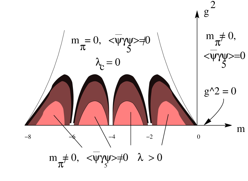
Figure 1: Schematic diagram of the quenched Aoki phase. A pionic condensate and corresponding non-zero density of near zero modes is developed throughout most of the negative mass region. In the coloured sectors, a non-zero mobility edge is developed and the contours could equally well represent either decreasing low mode density, decreasing pionic condensate or increasing $\lambda_{c}$ as one moves towards the continuum limit at $g^{2}=0$.

This qualitative picture is displayed in Figure 1. Following conventional terminology, we refer to the Aoki phase as that region of this diagram in which $\langle\overline{\psi}\gamma^{5}\tau^{a}\psi\rangle\neq 0$ and $g^{2}>g^{2}_{c}(-M_{5})$. In this region the coupling is sufficiently large that the mobility edge is zero and long-range correlations result from massless flavor-non-singlet pions. The near-zero modes of $H_{W}$ are delocalized. This is a dangerous region for chiral fermions, with lattice artifacts producing unphysical, long-distance correlations. For weaker coupling $g^{2}\leq g^{2}_{c}(-M_{5})$, these long-distance correlations have disappeared. The Wilson Dirac eigenvectors with low eigenvalues are localized on the lattice scale and all delocalized modes have eigenvalues which, if expressed in physical units, are at least as large as $\lambda_{c}(-M_{5})/a$. These delocalized low modes do not introduce unphysical non-locality into the corresponding formulation of lattice chiral fermions but, as discussed in the next section, they enhance the explicit violation of chiral symmetry for domain wall fermions with finite $L_{s}$.

III Low-lying spectrum of $H_{W}$ and lattice chiral fermions

We now discuss in more detail the relation between the spectrum of the hermitian Wilson Dirac operator $H_{W}$ and the properties of domain wall fermions. Let us first address the issue of locality. While the domain wall Dirac operator contains only nearest-neighbor couplings in five dimensions (i.e. is ultra-local), the four dimensional effective low energy theory which it produces may contain unphysical non-locality. One approach to investigating this question is to examine the locality of the overlap operator that results in the $L_{s}\rightarrow\infty$ limit Neuberger (1998b); Kikukawa and Noguchi (1999). This was done by Hernandez et al. Hernandez et al. (1999) using $H_{W}$ as the kernel in the sign function of the overlap operator. They showed that a gap in the spectrum of the eigenstates of $H_{W}$ guarantees locality of the resulting overlap operator. The proof relies on the ultra-local nature of $H_{W}$ implying ultra-locality of a finite polynomial of $H_{W}$. The “Shamir” kernel $K_{S}$ for the overlap operator that corresponds to the $L_{s}=\infty$ limit of domain wall fermions can be taken as $K_{S}=H_{W}(2+D_{W})^{-1}$ Borici (2000, 1999); Edwards and Heller (2001) and it is not manifestly ultra-local. However, the operator $2+D_{W}$ in the denominator of $K_{S}$ is the Wilson Dirac operator with a $2-M_{5}$ mass term and hence, provided $M_{5}<2$ is outside the super-critical region ensuring that this kernel is exponentially localized. The Hernandez et al. proof is therefore applicable to domain wall fermions under the modification that a finite polynomial of an exponentially local operator is also exponentially local.

However, as discussed above, the assumed gap in the spectrum of $H_{W}$ is neither expected nor observed in lattice QCD, at least for the range of couplings in which calculations are normally performed. Fortunately, as argued by Golterman et al. Golterman and Shamir (2003), the detailed properties of the Wilson Dirac operator in the super-critical region described above are sufficient to imply that the overlap operator is appropriately local (provided we are outside of the Aoki phase and $\lambda_{c}(-M_{5},g)>0$). If, as is the case in this picture, one assumes that the spectrum of extended states shows a gap (the region $0\leq\lambda\leq\lambda_{c}$) so that any eigenstates within the gap are localized, then the resulting overlap operator will also be localized (even though the density of low modes is non-zero). This is supported by numerical evidence at currently affordable couplings.

Finally, we examine a second difficulty faced by domain wall fermions and related approaches, which is closely connected with these low-lying modes of $H_{W}$. The residual chiral symmetry breaking effects seen at finite $L_{s}$ for domain wall fermions depend in detail on the densities and sizes of the modes of the hermitian matrix $H_{T}$. This is reviewed in Appendix A, and $H_{T}$ is defined in Eq. 64. $H_{T}$ is used to construct the Fock-space transfer matrix in the fifth dimension, $T$ defined in Eq. 57. This transfer matrix describes explicitly how the left and right walls are coupled when $L_{s}$ is finite. While the relation between the operators $H_{W}$ and $H_{T}$ is somewhat complex, it can be shown that their zero modes coincide Furman and Shamir (1995), and also that $-\log T\equiv H_{T}=2\tanh^{-1}K_{S}$, where $K_{S}=\frac{H_{W}}{2+D_{W}}$ Borici (2000, 1999); Edwards and Heller (2001). Further, the corresponding approximation to the overlap operator, and its $L_{s}\to\infty$ limit are: Neuberger (1998b)

$$\begin{array}[]{cccc}&D_{\rm ov}^{\rm approx}&=&\frac{1}{2}\left[1+m+(1-m)\gamma_{5}\tanh(\frac{L_{s}}{2}H_{T})\right]\\ \to&D_{\rm ov}&=&\frac{1}{2}\left[1+m+(1-m)\gamma_{5}{\rm sgn}H_{T})\right],\end{array}$$ (1)

or equivalently,

$$\begin{array}[]{cccc}&D_{\rm ov}^{\rm approx}&=&\frac{1}{2}\left[1+m+(1-m)\gamma_{5}\tanh(L_{s}\tanh^{-1}K_{S})\right]\\ \to&D_{\rm ov}&=&\frac{1}{2}\left[1+m+(1-m)\gamma_{5}{\rm sgn}K_{S})\right].\end{array}$$ (2)

The equality of the operators ${\rm sgn}H_{T}$ and ${\rm sgn}K_{S}$ follows easily from the relation $H_{T}=2{\rm tanh}^{-1}K_{S}$ and the recognition that the inverse hyperbolic tangent is a function which preserves the sign of its argument.

Thus, the near-zero modes of $H_{W}$ discussed above are expected to correspond to near-zero modes of $H_{T}$, modes which (in the absence of an explicit mass term) will dominate the coupling of the left- and right-handed sectors of low-energy domain wall QCD. Similarly, the mobility edge structure of $H_{W}$ is also expected to describe $H_{T}$. As is exploited in the next section, this implies a simple structure for the asymptotic $L_{s}$-dependence of the residual mass. The near-zero localized modes will give a power behavior ($1/L_{s}$), while the extended modes above the mobility edge give an exponential fall-off ($e^{-\lambda_{c}L_{s}}/L_{s}$). This dependence will be used as one of several diagnostics to investigate the nature of the $H_{T}$ spectrum in our simulations.

The strong-coupling behaviour of the Wilson Dirac operator does not leave one at liberty to simulate QCD at arbitrarily coarse lattice spacings. For a given lattice action, the phase boundary where the gap in the spectrum of extended states vanishes defines the coarsest lattice spacing at which the formulation makes sense and implies a minimum cost that must be paid to have the formulation under control. The phase boundary is action dependent and, in practice, we will wish to stay well within the phase such that the mobility edge is not small.

We have performed the first numerical study of the localization of the hermitian Wilson Dirac operator with three mass degenerate flavors of light dynamical quarks and demonstrate that a programme of 2+1 flavor dynamical DWF simulations of QCD is rendered affordable by our current QCDOC computer systems. These considerations are directly relevant for all chirally symmetric lattice QCD formulations, and we shall later illustrate the smooth connection between finite $L_{s}$ and the $L_{s}\to\infty$ overlap limit with numerical data for the plaquette. Our work has been presented at Lattice 2005 Antonio et al. (2006a), and later, while this paper was being completed, a broadly similar study was presented at Lattice 2006 using dynamical overlap fermions Yamada et al. (2006).

IV Residual mass

In this section we discuss the residual mass in some detail, including a careful discussion of its dependence on $L_{s}$ as predicted by the transfer matrix analysis of Furman and Shamir. As we will demonstrate and has been worked out previously Golterman and Shamir (2003); Golterman et al. (2005a, b); Svetitsky et al. (2006); Christ (2006); Antonio et al. (2006a), this dependence on $L_{s}$ permits the effects of both the localized near-zero modes and the extended modes above the mobility edge to be recognized. This gives useful information about the general character of chiral symmetry breaking as well as an understanding of the origin of the residual mass itself.

In the limit of small lattice spacing, or equivalently weak gauge coupling, the spectrum of the domain wall Dirac operator for a typical gauge background is expected to have a physical, four-dimensional component with eigenvalues $\lambda\sim\Lambda_{\rm QCD}$ as well as unphysical, five-dimensional states with $\lambda\sim 1/a$. The low-lying modes permit the accurate simulation of QCD while the large eigenvalues are lattice artifacts similar to, but more numerous than, the unphysical large eigenvalues found in other lattice fermion formulations. Ideally, the physical four-dimensional states will be bound near the $s=0$ and $s=L_{s}-1$ walls. To the extent that $L_{s}$ is large, there should be little mixing between the left-handed chiral states localized on the left ($s=0$) wall and the right-handed chiral states localized on the right ($s=L_{s}-1$) wall.

The low-energy properties of this approximately chiral theory can be described by an effective Lagrangian, ${\cal L}_{\rm eff}$. If effects coming from non-zero lattice spacing or arising from the overlap between the left- and right-handed states are neglected, this effective Lagrangian will be precisely that of QCD. The corrections coming from these effects can be described by adding extra operators to ${\cal L}_{\rm eff}$. The only relevant operator of this sort is a dimension-3 mass term. The next most important term is the familiar dimension-5 Sheikholeslami-Wohlert term. Thus,

$${\cal L}_{\rm eff}={\cal L}_{\rm QCD}+m_{\rm res}\overline{q}q+c_{5}\overline{q}\sigma^{\mu\nu}F^{\mu\nu}q+\ldots$$ (3)

In this paper we focus on the coefficient, $m_{\rm res}$, of this residual mass term as an important measure of the violation of chiral symmetry arising from the finite extent ($L_{s}$) in the fifth dimension. In this section, we will discuss the dependence of $m_{\rm res}$ on $L_{s}$ by using the transfer matrix formalism of Furman and Shamir Furman and Shamir (1995), described in Appendix A which is a prerequisite for those unfamiliar with this formalism.

IV.1 Transfer matrix in the fifth dimension

Using the transfer matrix approach, the approximate chiral symmetry of domain wall fermions is realized by writing a general Green’s function by semi-independent products of left- and right-handed operators. As is described in Appendix A, if we arrange the field variables appearing in a general Green’s function by segregating the left- and right-handed fields into two products, ${\cal O}_{L}[P_{L}q,\overline{q}P_{R}]$ and ${\cal O}_{R}[P_{R}q,\overline{q}P_{L}]$ then, we can write

$$\left\langle{\cal O}_{L}[P_{L}q,\overline{q}P_{R}]\;{\cal O}_{R}[P_{R}q,\overline{q}P_{L}]\right\rangle_{L_{s}}\hskip-36.135pt$$

$$=Z(L_{s})\;{\rm tr}\left\{{\cal O}_{L}[P_{L}\hat{a},-\hat{a}^{\dagger}P_{R}]\hat{T}^{L_{s}}{\cal O}_{R}[P_{R}\hat{a},\hat{a}^{\dagger}P_{L}]{\cal{O}}(m_{f})\right\}.$$

The left-hand side of this equation is a general, DWF Green’s function defined as a Grassmann integral over the 5-dimensional domain wall field variables $\overline{\Psi}(x,s)$ and $\Psi(x,s)$ using the usual DWF action, $S_{F}=-\overline{\Psi}D^{\rm DWF}\Psi$. Here the Grassmann fields $\overline{\Psi}(x,s)$ and $\Psi(x,s)$ are functions of a space-time coordinate $x$ and fifth-dimensional coordinate $s$, $0\leq s\leq L_{s}-1$. The domain wall Dirac operator $D^{\rm DWF}$ is that of Shamir Shamir (1993), and Furman and Shamir Furman and Shamir (1995) and in our notation is given by

$$D^{\rm DWF}_{x,s;x^{\prime},s^{\prime}}(M_{5},m_{f})=\delta_{s,s^{\prime}}D^{\parallel}_{x,x^{\prime}}(M_{5})+\delta_{x,x^{\prime}}D^{\bot}_{s,s^{\prime}}(m_{f})$$ (5)

$$D^{\parallel}_{x,x^{\prime}}(M_{5}) = {1\over 2}\sum_{\mu=1}^{4}\left[(1-\gamma_{\mu})U_{x,\mu}\delta_{x+\hat{\mu},x^{\prime}}+(1+\gamma_{\mu})U^{\dagger}_{x^{\prime},\mu}\delta_{x-\hat{\mu},x^{\prime}}\right]$$ (6)

$$+ (M_{5}-4)\delta_{x,x^{\prime}}$$

$$D^{\bot}_{s,s^{\prime}}(m_{f}) = {1\over 2}\Big{[}(1-\gamma_{5})\delta_{s+1,s^{\prime}}+(1+\gamma_{5})\delta_{s-1,s^{\prime}}-2\delta_{s,s^{\prime}}\Big{]}$$ (7)

$$- {m_{f}\over 2}\Big{[}(1-\gamma_{5})\delta_{s,L_{s}-1}\delta_{0,s^{\prime}}+(1+\gamma_{5})\delta_{s,0}\delta_{L_{s}-1,s^{\prime}}\Big{]}.$$

The physical four-dimensional Grassmann fields, $q(x)$ and $\overline{q}(x)$, are constructed from the five-dimensional fields $\overline{\Psi}(x,s)$ and $\Psi(x,s)$ according to Eqs. 65 and 66.

The right-hand side of Eq. IV.1 is the trace of a product of operators acting on a many-particle Fock space. In contrast to the usual field theory setting, these particles are located in a four-dimensional coordinate space. Thus, the fields $a_{x}$ and $a_{x}^{\dagger}$ depend on the space-time position $x$, as well as other spin and color indices which are not shown. These operators, as well as the transfer matrix $\hat{T}$, and mass operator ${\cal{O}}(m_{f})$, are defined in Appendix A. The factor $Z(L_{s})$ is an $L_{s}$-dependent normalization factor. The mass $M_{5}$ is the domain wall height. The mass $m_{f}$ is the bare mass of the physical fermions.

In the limit in which $m_{f}=0$ and $L_{s}\to\infty$, $\hat{T}^{L_{s}}$ is viewed as projecting onto the state with the largest eigenvalue (normalized to be unity), and the right-hand side of Eq. IV.1 becomes the product of two completely independent matrix elements corresponding to isolated left- and right-handed theories (see Eq. 84). This exact chiral symmetry is violated by the operator ${\cal{O}}(m_{f})$ which represents the explicit mass term and mixes the left- and right-handed factors. Similarly, the corrections to the asymptotic limit $\hat{T}^{L_{s}}\to|0_{H}\rangle\langle 0_{H}|$ of Eq. 85 introduce chiral symmetry breaking arising from finite $L_{s}$.

In the above discussion, and that to follow, we are ignoring the effects of anomalous chiral symmetry breaking. Such effects require modifications to our discussion for background gauge fields with non-zero Pontryagin index. For such gauge fields the state $|0_{H}\rangle$ will carrying a fermion number different from that of $|0_{S}\rangle$, thereby introducing flavor-singlet chirality correlations between the otherwise independent left and right-hand factors in the first term on the right-hand side of Eq. IV.1 Narayanan and Neuberger (1995). In the interests of simplicity, we do not consider such gauge configurations here. However, the effects of these configurations do not alter our conclusions.

IV.2 Residual mass and the transfer matrix

We will now explicitly study the first corrections to the large $L_{s}$ limit of $\hat{T}^{L_{s}}$ in Eq. IV.1 where, for clarity, we set $m_{f}=0$ and use the relation ${\cal{O}}(m_{f}=0)=|0_{S}\rangle\langle 0_{S}|$ discussed in Appendix A:

$$\left\langle{\cal O}_{L}[P_{L}q,\overline{q}P_{R}]{\cal O}_{R}[P_{R}q,\overline{q}P_{L}]\right\rangle_{L_{s}} = Z(L_{s})\;\langle 0_{S}|{\cal O}_{L}[P_{L}\hat{a},-\hat{a}^{\dagger}P_{R}]$$

$$\hskip-93.95122pt\Bigl{\{}|0_{H}\rangle\langle 0_{H}|+\sum_{k^{+}=1}^{N^{+}}e^{-E^{+}_{k^{+}}L_{s}}\hat{o}_{k^{+}}^{\dagger}|0_{H}\rangle\langle 0_{H}|\hat{o}_{k^{+}}+\sum_{k^{-}=1}^{N^{-}}e^{-E^{-}_{k^{-}}L_{s}}\hat{p}_{k^{-}}^{\dagger}|0_{H}\rangle\langle 0_{H}|\hat{p}_{k^{-}}\Bigr{\}}$$

$$\hskip 72.26999pt{\cal O}_{R}[P_{R}\hat{a},\hat{a}^{\dagger}P_{L}]|0_{S}\rangle.$$

Here the leading term, the projection operator $|0_{H}\rangle\langle 0_{H}|$, divides the Green’s function into two independent factors demonstrating the separate flavored chiral symmetry of the left- and right-handed fermions. The first correction permits quark number $\pm 1$ exchanges between these two otherwise independent sectors. This suggests that the second and third terms in Eq. IV.2 should be interpreted at low energies as the residual mass operator $m_{\rm res}\overline{q}q$ expressed in this 5-dimensional language.

A relation between this residual mass term and the second and third terms in the operator in curly brackets in Eq. IV.2 can be obtained if we express the operators $\hat{o}_{k}$ and $\hat{p}_{k}$ in terms of the conventional 4-dimensional field $\hat{a}_{x}$, inverting Eq. 74:

$$-\sum_{n}m_{\rm res}\overline{q}(x_{n})q(x_{n})\rightarrow m_{\rm res}\sum_{n}\Bigl{\{}(\hat{a}^{\dagger}_{x_{n}}P_{R})_{\alpha}|0_{H}\rangle\langle 0_{H}|(P_{R}\hat{a}_{x_{n}})_{\alpha}$$

$$\hskip 36.135pt+(P_{L}\hat{a}_{x_{n}})_{\alpha}|0_{H}\rangle\langle 0_{H}|(\hat{a}^{\dagger}_{x_{n}}P_{L})_{\alpha}\Bigr{\}}$$

$$\mathrel{\mathop{\approx}^{?}} \sum_{k}\sum_{n,n^{\prime}}\phi^{+}_{k\alpha}(x_{n})\phi^{+}_{k\beta}(y_{n^{\prime}})^{*}e^{-L_{s}E_{k}^{+}}\;(\hat{a}_{x_{n}}^{\dagger}P_{R})_{\alpha}|0_{H}\rangle\langle 0_{H}|(P_{R}\hat{a}_{y_{n^{\prime}}})_{\beta}$$

$$+ \sum_{k}\sum_{n,n^{\prime}}\phi^{-}_{k\alpha}(x_{n})^{*}\phi^{-}_{k\beta}(y_{n^{\prime}})e^{-L_{s}E_{k}^{-}}\;(P_{L}\hat{a}_{x_{n}})_{\alpha}|0_{H}\rangle\langle 0_{H}|(\hat{a}_{y_{n^{\prime}}}^{\dagger}P_{L})_{\beta}.$$

Here the RHS of Eq. IV.2 is the usual residual mass term, $-m_{\rm res}\overline{q}q$, written in the transfer matrix language (see Eq. A), while the expression in Eq. LABEL:eq:m_res_def1 is a version of the leading order contribution from the second and third terms in Eq. IV.2. The projection operators $P_{R}$ and $P_{L}$ can be introduced into the right-hand side of Eq. LABEL:eq:m_res_def1 because the other chirality will vanish in the limit $m_{f}=0$ .

We can justify this relation and estimate $m_{\rm res}$ if we assume that the sums $\sum_{k}\phi^{\pm}_{k}(x_{n})^{\dagger}\phi^{\pm}_{k}(y_{n^{\prime}})$ are localized on the long distance scale at which $m_{\rm res}$ is defined:

$$K_{\alpha,\beta}(x,y)=\sum_{k}\phi^{\pm}_{k,\alpha}(x)^{\dagger}\phi^{\pm}_{k,\beta}(y)e^{-L_{s}E_{k}^{\pm}}\approx m_{\rm res}\delta^{4}(x-y)\delta_{\alpha,\beta}\,,$$ (11)

where $\alpha$ and $\beta$ are each spin and color indices, and we assume that the diagonal spin/color structure will appear and any dependence on the label $\pm$ will disappear when a volume and/or gauge average is performed. We can then approximate: $m_{\rm res}=\frac{1}{12}\int d^{4}xK_{\alpha,\alpha}(x,y)\approx\frac{1}{12}R^{4}K_{\alpha,\alpha}(y,y)$, where the “radius” $R$ estimates the small region in $x$ that contributes and summation is performed over the repeated spin and color index $\alpha$. Finally, $K(y,y)$ and hence $m_{\rm res}$ can be determined by integrating over $y$ and using the orthonormality of the eigenfunctions $\phi^{\pm}_{k\alpha}(y)$:

$$m_{\rm res} = \frac{R^{4}}{12}K_{\alpha,\alpha}(y,y)=\frac{R^{4}}{12L^{3}L_{t}}\int d^{4}yK_{\alpha,\alpha}(y,y)$$ (12)

$$= \frac{R^{4}}{12L^{3}L_{t}}\sum_{k}e^{-L_{s}E_{k}^{\pm}}=R^{4}\int_{0}^{\infty}d\lambda\rho(\lambda)e^{-L_{s}\lambda}$$ (13)

$$\sim R_{e}^{4}\rho_{e}(\lambda_{c})\frac{e^{-\lambda_{c}L_{s}}}{L_{s}}+R_{l}^{4}\rho_{l}(0)\frac{1}{L_{s}}.$$ (14)

Here $\rho(\lambda)$ on the RHS of Eq. 13 is the density of eigenvalues of $H_{T}$ per unit space-time volume, color and spin. The final Eq. 14 is a generalization of Eq. 13 displaying the expected contributions of extended ($e$) and localized ($l$) modes with possibly different radius parameters, $R_{l}$ and $R_{e}$. Eq. 14 should be viewed as a theoretically motivated model for the large $L_{s}$ behavior of the residual mass where $R_{l}$ is the radius of the localized states with eigenvalue close to zero. The radius associated with the extended states, $R_{e}$, arises from the limited spatial resolution provided by a sum over extended states resulting from the high-momentum cutoff intrinsic to the lattice formulation. This suggests $R_{e}\approx a$. In this final equation we have also taken the limit of large $L_{s}$ to simplify the integral over $\lambda$. This is the “standard” result for the dependence of $m_{\rm res}$ on $L_{s}$, although the factor of $1/L_{s}$ is usually missing from the left-most term. We will use Eq. 14 elsewhere in this paper to interprete the dependence of $m_{\rm res}$ on $L_{s}$.

IV.3 Residual mass and the 5-dimensional axial current

While the above discussion provides a direct connection between corrections to the $L_{s}\to\infty$ limit and the residual mass, it does not give a simple way to compute $m_{\rm res}$. This is typically done using a partially conserved 5-dimensional axial current introduced by Furman and Shamir Furman and Shamir (1995):

$${\cal A}^{b}_{\mu}(x)=\sum_{s=0}^{L_{s}-1}{\rm sign}(s-\frac{L_{s}-1}{2})j^{b}_{\mu}(x,s),$$ (15)

where the current $j^{b}_{\mu}(x,s)$ is defined by

$$j^{b}_{\mu}(x,s)=\frac{1}{2}\left[\overline{\Psi}(x+\hat{\mu},s)(1+\gamma_{\mu})U^{\dagger}_{x+\mu,\mu}t^{b}\Psi(x,s)-\overline{\Psi}(x,s)(1-\gamma_{\mu})U_{x,\mu}t^{b}\Psi(x+\mu,s)\right],$$ (16)

and $b$ is a flavor index and $t^{b}$ is a generator of the flavor symmetry. The equations of motion imply the conservation law

$$\Delta_{\mu}{\cal A}^{b}_{\mu}(x)=2m_{f}\overline{q}(x)t^{b}\gamma^{5}q(x)+J^{b}_{5q}(x)$$ (17)

where $J^{b}_{5q}$ is defined in Eq. 69 and we define $(\Delta_{\mu}f)(x)=f(x)-f(x-\hat{\mu})$.

In the limit of large $L_{s}$ and small lattice spacing, the extra $J^{b}_{5q}$ term in the conservation law in Eq. 17 should describe the chiral asymmetry of the leading dimension-3 term in the domain wall fermion effective Lagrangian, $m_{\rm res}\overline{q}q$:

$$J^{b}_{5q}\approx 2m_{\rm res}\overline{q}t^{b}\gamma^{5}q.$$ (18)

This equation can be used directly to determine $m_{\rm res}$ by evaluating the ratio of the matrix elements of $J^{b}_{5q}$ and $\overline{q}t^{b}\gamma^{5}q$. In this paper, we use the ratio of pion correlation functions:

$$m_{\rm res}=\frac{\langle J^{b}_{5q}(x)\;\overline{q}t^{b}\gamma^{5}q(y)\rangle}{\langle 2\overline{q}t^{b}\gamma^{5}q(x)\;\overline{q}t^{b}\gamma^{5}q(y)\rangle}$$ (19)

evaluated for $|x-y|>>a$ to determine $m_{\rm res}$ numerically.

As a consistency check, we should demonstrate that the definitions of $m_{\rm res}$ given in Eqs. LABEL:eq:m_res_def1 and 18 agree. We begin by generalizing Eq. 71 to express a general Green’s function of $J^{b}_{5q}(z)$ with other physical fields, in a form in which the latter are separated into the left- and right-handed factors ${\cal O}_{L}[P_{L}q,\overline{q}P_{R}]$ and ${\cal O}_{R}[P_{R}q,\overline{q}P_{L}]$:

$$\langle{\cal O}_{L}[P_{L}q,\overline{q}P_{R}]J^{b}_{5q}(z){\cal O}_{R}[P_{R}q,\overline{q}P_{L}]\rangle$$ (20)

$$\hskip-144.54pt=Z(L_{s})\langle 0_{S}|{\cal O}_{L}[P_{L}\hat{a},-\hat{a}^{\dagger}P_{R}]\hat{T}^{\frac{L_{s}}{2}}\hat{a}^{\dagger}_{z}t^{b}\hat{a}_{z}\hat{T}^{\frac{L_{s}}{2}}{\cal O}_{R}[P_{R}\hat{a},\hat{a}^{\dagger}P_{R}]|0_{S}\rangle.$$

Since we wish to compare with Eqs. IV.2 and LABEL:eq:m_res_def1, we can simplify this expression by integrating the position variable $z$ over space-time:

$$Z(L_{s})\langle 0_{S}|{\cal O}_{L}[P_{L}\hat{a},-\hat{a}^{\dagger}P_{R}]\hat{T}^{\frac{L_{s}}{2}}\Bigl{\{}\sum_{k^{+}=1}^{N^{+}}\hat{o}^{\dagger}_{k^{+}}t^{b}\hat{o}_{k^{+}}-\sum_{k^{-}=1}^{N^{-}}\hat{p}^{\dagger}_{k^{-}}t^{b}\hat{p}_{k^{-}}\Bigr{\}}\hat{T}^{\frac{L_{s}}{2}}{\cal O}_{R}[P_{R}\hat{a},\hat{a}^{\dagger}P_{R}]|0_{S}\rangle.$$ (21)

Here we have also replaced the operators $\hat{a}_{x}$ and $\hat{a}_{x}^{\dagger}$ with those creating eigenstates of $\hat{T}$, using the definition in Eq. 74 and the orthogonality relations obeyed by the coefficients $\phi_{k^{\pm}}^{\pm}$. Next, we can evaluate the factors $\hat{T}^{\frac{L_{s}}{2}}$ in the limit of large $L_{s}$ using Eq. 85. The leading contribution to Eq. 21 results when the next leading contribution to $\hat{T}^{\frac{L_{s}}{2}}$ (the second and third terms in Eq. 85) is substituted for each factor:

$$Z(L_{s})\langle 0_{S}|{\cal O}_{L}[P_{L}\hat{a},-\hat{a}^{\dagger}P_{R}]\Bigl{(}\sum_{k_{1}^{+}=1}^{N^{+}}e^{-E^{+}_{k_{1}^{+}}\frac{L_{s}}{2}}\hat{o}_{k_{1}^{+}}^{\dagger}|0_{H}\rangle\langle 0_{H}|\hat{o}_{k_{1}^{+}}+\sum_{k_{1}^{-}=1}^{N^{-}}e^{-E^{-}_{k_{1}^{-}}\frac{L_{s}}{2}}\hat{p}_{k_{1}^{-}}^{\dagger}|0_{H}\rangle\langle 0_{H}|\hat{p}_{k_{1}^{-}}\Bigr{)}$$

$$\hskip-361.34999pt\Bigl{\{}\sum_{k^{+}=1}^{N^{+}}\hat{o}^{\dagger}_{k^{+}}t^{b}\hat{o}_{k^{+}}-\sum_{k^{-}=1}^{N^{-}}\hat{p}^{\dagger}_{k^{-}}t^{b}\hat{p}_{k^{-}}\Bigr{\}}$$

$$\hskip-433.62pt\Bigl{(}\sum_{k_{2}^{+}=1}^{N^{+}}e^{-E^{+}_{k_{2}^{+}}\frac{L_{s}}{2}}\hat{o}_{k_{2}^{+}}^{\dagger}|0_{H}\rangle\langle 0_{H}|\hat{o}_{k_{2}^{+}}+\sum_{k_{2}^{-}=1}^{N^{-}}e^{-E^{-}_{k_{2}^{-}}\frac{L_{s}}{2}}\hat{p}_{k_{2}^{-}}^{\dagger}|0_{H}\rangle\langle 0_{H}|\hat{p}_{k_{2}^{-}}\Bigr{)}{\cal O}_{R}[P_{R}\hat{a},\hat{a}^{\dagger}P_{L}]|0_{S}\rangle.$$

Exploiting the simple form of the operator in the curly brackets, Eq. IV.3 can be considerably simplified, yielding:

$$Z(L_{s})\langle 0_{S}|{\cal O}_{L}[P_{L}\hat{a},-\hat{a}^{\dagger}P_{R}]$$

$$\hskip-108.405pt\Bigl{\{}\sum_{k^{+}=1}^{N^{+}}e^{-E^{+}_{k^{+}}L_{s}}\hat{o}_{k^{+}}^{\dagger}|0_{H}\rangle t^{b}\langle 0_{H}|\hat{o}_{k^{+}}-\sum_{k^{-}=1}^{N^{-}}e^{-E^{-}_{k^{-}}L_{s}}\hat{p}_{k^{-}}^{\dagger}|0_{H}\rangle t^{b}\langle 0_{H}|\hat{p}_{k^{-}}\Bigr{\}}{\cal O}_{R}[P_{R}\hat{a},\hat{a}^{\dagger}P_{L}]|0_{S}\rangle$$

where the flavor generator $t^{b}$ acts on the suppressed flavor indices carried by the operators $\hat{o}_{k^{+}}^{\dagger}$, $\hat{o}_{k^{+}}$, $\hat{p}_{k^{-}}^{\dagger}$ and $\hat{p}_{k^{-}}$. Now we can directly compare the operator appearing in curly brackets in Eq. IV.3 (which should reduce to the operator $2m_{\mathrm{res}}\overline{q}t^{b}\gamma^{5}q$ at low energies) with the second and third terms of the operator in curly brackets in Eq. IV.2 (which we have shown does reduce to the operator $m_{\mathrm{res}}\overline{q}q$ in this limit). These two operators are directly related at first order in $\delta$ by an infinitesmal chiral transformation where operators in the left-hand factor transform as

$$\hat{o}_{k^{+}}^{\dagger}\rightarrow\hat{o}_{k^{+}}^{\dagger}(1+i\delta t^{b})\quad\quad\hat{p}_{k^{-}}^{\dagger}\rightarrow\hat{p}_{k^{-}}^{\dagger}(1-i\delta t^{b})$$ (24)

while operators in the right-hand factor transform as

$$\hat{o}_{k^{+}}\rightarrow(1+i\delta t^{b})\hat{o}_{k^{+}}\quad\quad\hat{p}_{k^{-}}\rightarrow(1-i\delta t^{b})\hat{p}_{k^{-}}.$$ (25)

Since this relation between the operators in curly brackets in Eqs. IV.3 and IV.2 will continue to hold in the long distance limit, each limiting quantity, $2m_{\mathrm{res}}\overline{q}t^{b}\gamma^{5}q$ and $m_{\mathrm{res}}\overline{q}q$, must contain the same value of $m_{\mathrm{res}}$. Thus, the residual mass defined in Eq. 19 agrees with that appearing in the residual mass operator deduced from the large $L_{s}$ limit of the transfer matrix for the case $m_{f}=0$. This demonstrates the expected consistency with a Symanzik effective Lagrangian description of the low-energy effects of mixing between the $s=0$ and $s=L_{s}-1$ walls.

V Lattice Actions and Ensembles

Our simulations have been performed with three flavors of dynamical DWF for a class of improved gauge actions. Our notation is the same as in Blum et al. (2004); Aoki et al. (2004, 2005), which we briefly review here. The partition function we simulate is

$$Z=\int[dU]\int\prod_{i=1}^{3}[d\Psi_{i}d\bar{\Psi}_{i}]\int\prod_{i=1}^{3}[d\Phi^{\dagger}_{{\rm PV},i}d\Phi_{{\rm PV},i}]e^{-S},$$ (26)

where the index $i$ runs over the up, down and strange quarks. The Pauli-Villars fields $\Phi_{{\rm PV},i}$ are needed to cancel the bulk infinity that would be produced by DWF as $L_{s}\to\infty$. In particular, the total action is

$$S=S_{G}(U)+S_{F}(\bar{\Psi},\Psi,U)+S_{PV}(\Phi^{\dagger},\Phi,U).$$ (27)

The gauge actions we consider are of the form

$$S_{\rm G}[U]=-\frac{\beta}{3}\left[(1-8\,c_{1})\sum_{x;\mu<\nu}P[U]_{x,\mu\nu}\\ +c_{1}\sum_{x;\mu\neq\nu}R[U]_{x,\mu\nu}\right]$$ (28)

where $P[U]_{x,\mu\nu}$ and $R[U]_{x,\mu\nu}$ represent the real part of the trace of the path ordered product of link variables around the $1\times 1$ plaquette and the $1\times 2$ rectangle, respectively, in the $\mu,\nu$ plane at the point $x$, and $\beta\equiv 6/g^{2}$ with $g$ the bare quark-gluon coupling. We use two common choices for $c_{1}$:

• the Iwasaki action which sets $c_{1}=-0.331$ Iwasaki (1985); Iwasaki and Yoshie (1984); and

• the DBW2 action which has $c_{1}=-1.4069$ Takaishi (1996); de Forcrand et al. (2000).

Both are known to reduce the residual mass very effectively in the quenched case.

The fermion action in Eq. 27 can be expressed in a form very close to the way it appears in the 3-flavor numerical work if it is written as:

$$S_{F}=-\sum_{i=1}^{3}\bar{\Psi}_{i}\left[D_{\rm DWF}^{\dagger}(M_{5},m_{i})D_{\rm DWF}(M_{5},m_{i})\right]^{1/2}\Psi_{i}$$ (29)

where $m_{i}$ is the input bare quark mass for the $i$th light quark flavor and the DWF Dirac operator $D_{\rm DWF}$ is defined in Eq. 5. We only consider the case where all light quarks have the same value for the five-dimensional domain-wall height, $M_{5}$. The action for the Pauli-Villars fields is similar, except that the quark mass $m_{i}$ is replaced by 1, to yield

$$S_{PV}=\sum_{i=1}^{3}\Phi^{\dagger}_{i}\left[D^{\dagger}_{\rm DWF}(M_{5},1)D_{\rm DWF}(M_{5},1)\right]^{1/2}\Phi_{i}.$$ (30)

The resulting determinants are suitable for simulation using a weight

$$\prod_{i}\frac{\det^{1/2}\left[D_{\rm DWF}^{\dagger}(M_{5},m_{i})D_{\rm DWF}(M_{5},m_{i})\right]}{\det^{1/2}\left[D_{\rm DWF}^{\dagger}(M_{5},1)D_{\rm DWF}(M_{5},1)\right]}.$$ (31)

The action may be simulated using either the inexact R algorithm Gottlieb et al. (1987), with associated step size errors, or the exact RHMC algorithm of Clark and Kennedy Clark and Kennedy (2007a, b). For the RHMC simulations, each of the square root factors in Eq. 31 are approximated by a rational function accurate over some eigenvalue range. Thus our simulation uses a 1+1+1 framework that happens to be mass degenerate. Where our mapping of the Aoki phase finds a clearly non-zero mobility edge it should be relevant to our more general programme of 2+1 flavour simulations where a chiral limit is taken in mass degenerate up/down quark masses at fixed strange mass. When written as a partial fraction expansion, each term is individually amenable to the usual HMC pseudo-fermionic integral (though, of course, a single pseudo-fermion and multi-mass inverter is used for all terms in the partial fraction expansion). We used the R algorithm for the earlier runs in our parameter search and used the RHMC out of preference, as documented in Table 1. Our implementation of the RHMC used separate fields as stochastic estimators of the numerator and denominator of Eq. 31. We simulated all three flavors in the numerator as separate single-flavor species, and treated the Pauli Villar fields as seperately estimated two- and single-flavour pseudofermions. Thus, we did not make any explicit use of the mass degeneracy between up and down quarks, (as would have been the case, for example, in two-flavor HMC).

The ensembles used in this study are a subset of those presented in Antonio et al. (2006b, c, d), and have been used for precision valence measurements with $L_{s}=8$. We used a reduced statistic subset to perform a consistent study as we vary $L_{s}$ in the (still expensive) valence analysis. The larger statistical sample used for the $L_{s}=8$ data points in Antonio et al. (2006b, c, d) lead to lower errors on results for $m_{\rm res}$ than we present in this work. We include only lower precision values in this paper to keep the $L_{s}=8$ analysis identical in all systematic respects to the $L_{s}>8$ points that are unique to this work. The ensembles used in this work are listed in Table 1. For the full simulation details, we refer the reader to Antonio et al. (2006b, c, d) where the entire dataset is presented.

All ensemble and correlation function computations were performed using the Columbia Physics System (CPS) on QCDOC computers in Edinburgh and Brookhaven. All measurements of four-dimensional eigenmodes were performed using the CHROMA physics system Edwards and Joo (2005), while the 5-dimensional modes were measured using CPS. The relation between these modes provides a non-trivial cross-check between code bases. Both code bases made use of the optimized Bagel QCD library Boyle . Visualization was carried out using the OpenDX software package.

VI Spectrum of the Hermitian Wilson Dirac Operator

In this section we study the eigenspectrum and eigenmodes of $H_{W}$ on our ensembles. We determined up to 256 eigenvectors of $H_{W}$ on 25 configurations per ensemble, at the negative mass $M_{5}=1.8$ that was used in our domain wall action for the sea quarks. Additional eigenvalues were generated on a number of configurations as a function of $M_{5}$. Our study therefore includes the dependence of the low-lying spectrum on $M_{5}$, often called spectral flows, in Section VI.1. We also study the spectral density of near-zero modes in Section VI.2, the microscopic shape distribution of the low-lying modes in Section VI.3, and the relation between modes of the hermitian 5-dimensional operator $H_{\rm DWF}=\gamma_{5}R_{5}D_{\rm DWF}$ and $H_{W}$ in Section VI.4, where $R_{5}$ is the reflection operator in the fifth dimension.

VI.1 Spectral flows

Prior to recent work on localization, it was believed that a gap in the spectrum was required for the correct behaviour of the various lattice formulations of chiral symmetry. In this context, it was believed that by obtaining spectral flows of the lowest few modes on a “typical” configuration, the health of the formulation was indicated by a nicely opened “eye” for some range of $M_{5}$ containing the Wilson mass used in the simulation. Recent improved understanding suggests that a non-zero, but low, density of localized states exists throughout the region in which we can afford to simulate. A gap, as such, does not exist after an ensemble average and, if spectral flows from sufficiently many configurations were overlaid, the entire eye would be filled in.

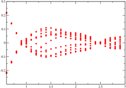
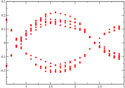
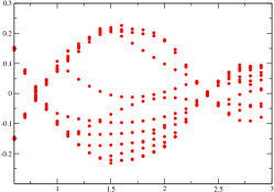
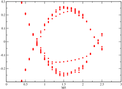
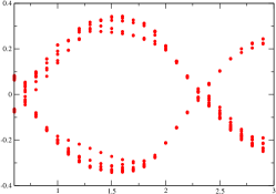
Figure 2: Spectral flow of DBW2. The horizontal axis is the valence domain wall height, $0\leq M_{5}\leq 3.0$ and the vertical axis is the eigenvalue of $H_{W}$, $-0.3\leq\lambda_{H_{W}}\leq 0.3$. From left, $\beta=0.72,,\beta=0.764,\beta=0.78$ (first row) and $\beta=0.8,\beta=0.88$ (second row).

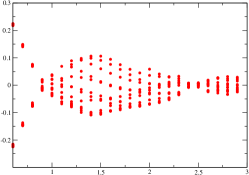
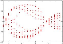
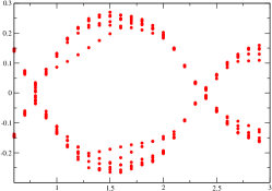
Figure 3: Spectral flow of Iwasaki $\beta=2.13,\beta=2.2$, and $\beta=2.3$ (from left to right). Axes are the same as fig 2.

However, on a small sample of configurations an open eye is indicative of a low density of low-lying modes and, we argue, a non-zero mobility edge since our results show that the spectral density grows rapidly across this edge. The flows presented here also allow comparison between our ensembles and those of previous works. These plots for the lowest modes, Figures 2 and 3, are therefore useful information at the larger values of $\beta$ where the open eye is indicative of a non-zero lower bound for the mobility edge, as presented previously Antonio et al. (2006e).

Our spectral flow results are certainly indicative of a non-zero mobility edge for $\beta\geq 0.78$ for the DBW2 gauge action and $\beta\geq 2.2$ for the Iwasaki gauge action. For smaller values of $\beta$ the spectral flows are inconclusive as no opening is displayed suggesting a non-zero density of low modes. We shall return to look at the localization structure in a more sophisticated fashion and classify these modes in Section VI.3.

VI.2 Spectral density

For each dataset comprising $n_{\rm conf}$ configurations we label the $i$th eigenvalue on the $j$th configuration $\lambda_{ij}$. We use a somewhat simplistic binning approach to estimate the spectral density for a partitioning of the spectrum. For the $k$th bin we estimate the density as

$$\rho^{k}([\lambda^{k}_{\rm min}+\lambda^{k}_{\rm max}]/2)=\frac{1}{n_{\rm conf}}\frac{N_{k}}{\lambda^{k}_{\rm max}-\lambda^{k}_{\rm min}},$$

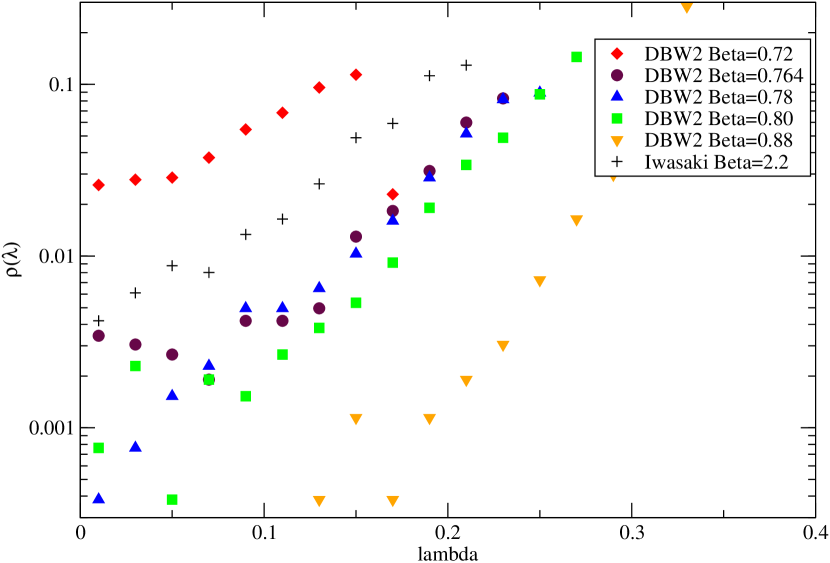
Figure 4: Spectral density obtained on a subset of our data with no error analysis, and fixed bin width $0.02$. Thus, where the density is low the error could be large and the data should be considered only as a qualitative indication of the nature of our ensembles.

where $N_{k}$ is the number of eigenvalues $\lambda_{ij}\in[\lambda^{k}_{\rm min}+\lambda^{k}_{\rm max}],j=1,\ldots,n_{\rm conf}$. Figure 4 displays our results for the spectral densities for our various datasets, using a fixed bin width of 0.02. Some clear, and unsurprising, trends are evident: the spectral density $\rho(0)$ is non-zero, and falls rapidly as $\beta$ is increased. The quantity $\rho(0)$ is slightly higher for the Iwasaki action at $\beta=2.2$ than for DBW2 at $\beta=0.78$ which have comparable lattice spacings. The density $\rho(\lambda)$ rises rapidly, and perhaps exponentially, in $\lambda$ as we move away from zero.

VI.3 Microscopic study of the mobility edge

We wish to study the size distribution of our eigenvectors, $\psi(x)$, as a function of the eigenvalue in order to test the mobility edge conjecture. This approach is novel and was first presented in Antonio et al. (2006a) for dynamical DWF, with a similar approach taken in Yamada et al. (2006) for dynamical overlap. A standard measure is the inverse participation ratio,

$$P^{-1}=\sum\limits_{x}|\psi^{\dagger}(x)\psi(x)|^{2}.$$

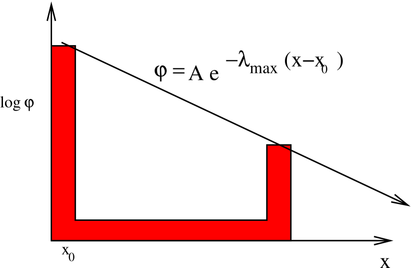
Figure 5: Various measures can be used to define the degree of localization. Inverse participation ratio has been a popular order parameter for delocalization transitions and, while fine for that purpose, counts occupied sites without paying attention to mode shape. This one dimensional cartoon highlights the advantages of the more robust measure employed in this paper. Given the model of exponential localization, our tactic is to find a localization exponent that forms a tight bound for the eigenvector. This measure will show the influence of satellite peaks in a robust fashion by eliminating all forms of dilution by volume average. Other useful measures that take into account the shape would include appropriately weighted moments of the density function.

A normalized extended state will produce $P\simeq V$, while a completely localized state will produce $P\simeq 1$. Thus the (inverse) participation ratio essentially counts the number of occupied sites and, in the infinite volume limit, is a useful order parameter for delocalization transitions. However, this metric is not sensitive to the shape of a state and so makes no distinction between occupying two adjacent sites, and occupying two well separated sites, such as the illustrative non-local example in Figure 5.

We want to understand how to reliably distinguish exponentially compact states from those with any degree of long-range support. In the infinite volume limit the use of the inverse participation ratio only identifies long-range correlations arising from structures whose four dimensional volume diverges and we seek a more robust measure.

While a better measure could be a moment of the eigenvector density, such as

$$\sum\limits_{x}\psi^{\dagger}(x)\psi(x)|x|,$$

we have found empirically, by visualizing data, that near the delocalization threshold the dominant long range correlation arises from multi-peaked eigenvectors, which fall exponentially around multiple centers. We define a more robust measure of exponential localization length, which generalizes the one dimensional case of Figure 5 to higher dimensions as follows

• The mode density is defined as $\phi(x)=\psi^{\dagger}(x)\psi(x)$.

• We identify a center $x_{0}$ such that $\phi(x_{0})\geq\phi(x)\forall x\neq x_{0}$.

• For every site, we define a radius $r(x)=|x-x_{0}|$ using the periodic mirror image nearest to $x_{0}$.

• We define an effective localization exponent $L_{\rm eff}(x)=\frac{2r(x)}{\log\phi(x_{0})-\log\phi(x)}$.

• Finally, we define a robust localization length $L_{\rm max}=\max\limits_{r(x)\geq 5}L_{\rm eff}(x)$.

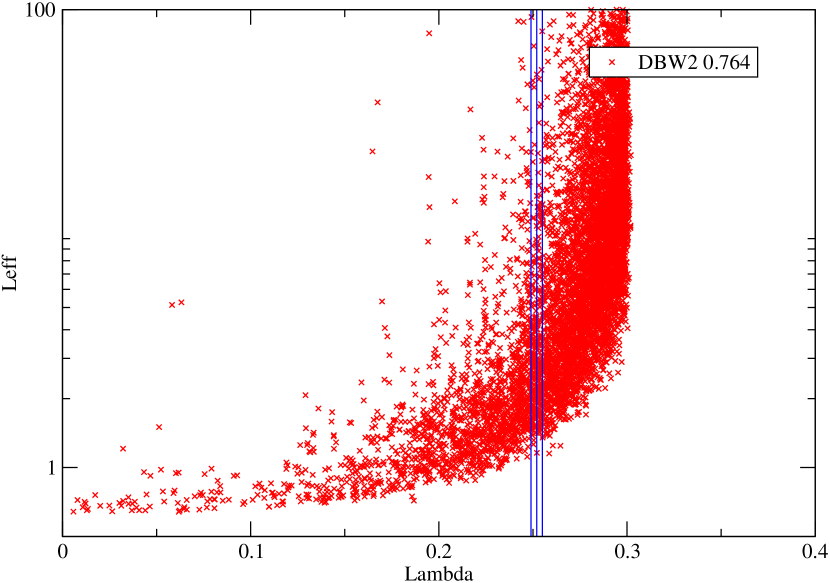
Figure 6: Microscopic view of the mobility edge based on a scatter plot of maximal localization lengths of individual low eigenmodes of $H_{W}$. We overlay the $H_{T}$ mobility edge $\lambda_{c}$ from fits to the model for $m_{\rm res}$, Eq 35 and find good agreement with our diverging localisation length for the DBW2 gauge action at $\beta=0.764$.

As the eigenvalue approaches the mobility edge from below, we observed two clear processes by which delocalization takes place. Firstly, the mean rate of fall off from the center decreases creating much bigger states. Secondly, states become increasingly multi-centered, with exponential fall off between a number of satellite peaks. The above definition of localization length is designed to reflect both the process of single-peak broadening, and the development of multiple peaks. The inverse participation ratio would be a less robust measure of locality in that it would not differentiate two well-separated $\delta$ functions from those on two neighbouring sites, or indeed would not identify a lower-dimensional extended sheet in the infinite volume. We display scatter plots of this definition of localization length for the 256 lowest eigenvectors of $H_{W}$ on 25 configurations per ensemble in Figure 6 and 7 for the DBW2 and Iwasaki gauge actions at $\beta=2.13$ and $\beta=0.764$ respectively.

VI.4 Relation between eigenmodes of the five and four-dimensional operators

We computed the lowest 10 modes of the 5-dimensional hermitian domain wall operator $H_{\rm DWF}=\gamma_{5}R_{5}D_{\rm DWF}$, using the Columbia Physics System, on a single configuration from a $16^{3}\times 32\times 8$ DBW2 three flavor ensemble at $\beta=0.764$. On the same configuration, we used the lowest 256 eigenmodes $\psi_{j}(x)$ of $H_{W}$, computed using the CHROMA software package, to express the 5-dimensional modes $\Psi_{i}(x,s)$ as a sum over 4-dimensional modes using

$$\Psi_{i}(x,s)=N_{s}\sum_{j}\alpha_{ij}(s)\psi_{j}(x),$$ (32)

where

$$N_{s}^{2}=\sum_{x}\Psi_{i}^{\dagger}(x,s)\Psi_{i}(x,s)$$

normalizes each $s$-slice of the 5-dimensional eigenvector to unity. This means that if the basis of 4-dimensional eigenvectors were complete

$$\sum_{j}\alpha_{ij}(s)^{2}=1.$$ (33)

However, since we are only using the lowest 256 eigenmodes, we expect that Eq. 32 will, at best, be true only deep in the bulk for large $L_{s}$ where low modes of the transfer matrix dominate, and only up to differences between $H_{T}$ and $H_{W}$.

We therefore computed 5-dimensional modes for a valence $L_{s}=16$ (N.B. not the unitary $L_{s}=8$ case) finding that, while the basis is very much incomplete on the wall, the description it gives in the 5-dimensional bulk is as much as 80% complete by the mid-point, despite the mismatch between $H_{T}$ and $H_{W}$. (This also serves as a useful cross check between the eigensolvers in the two independent code bases.)

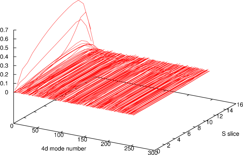
Figure 10: Normalized overlap of different $s$-slices of a chiral 5-dimensional eigenmode of $H_{DWF}$ with the first 256 4-dimensional eigenmodes of $H_{W}$. We take the valence operator with $L_{s}=16$, and demonstrate numerically that only a few low-lying 4-dimensional eigenmodes dominate the large $L_{s}$ contributions to chirality mixing operators such as $m_{\rm res}$ by plotting the decomposition of the lowest 5-dimensional mode $|\alpha_{0j}(s)|^{2}$ as a function of fifth coordinate $s$, and 4-dimensional mode number $j$.

The coefficients $|\alpha_{ij}|^{2}$ for a typical 5-dimensional chiral mode are displayed in Figure 10 and it can be seen that only 3 low-lying modes of $H_{W}$ dominate the $s$-dependence of eigenmodes of $H_{\rm DWF}$. Thus, we clearly demonstrate from numerical data that a few localized low-lying 4-dimensional modes of $H_{W}$ almost completely describe the coupling between walls for each 5-dimensional mode of the hermitian DWF operator for large $L_{s}$. As discussed, these modes occur with a low density - perhaps a “dilute gas” is an appropriate picture - but, for sufficiently large $L_{s}$, they dominate the contributions to chiral symmetry breaking due to exponential suppression of the extended modes above the mobility edge, see Eq. 14.

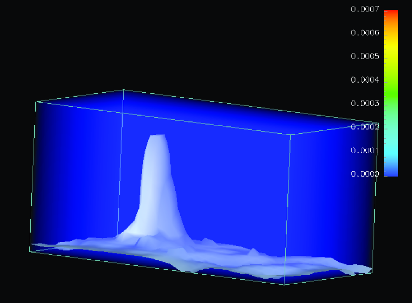
Figure 8: We display an iso-surface through the eigenvector density of a typical near-zero chiral mode of the 5-dimensional operator $H_{\rm DWF}$, bound to a single wall. Here $s$ is the vertical direction, $t$ the left-right axis, and $z$ runs into the page. We show $(x,y)=(3,3)$ showing a localized incursion of the eigenmode into the fifth dimension associated with a low mode of $H_{W}$. This mechanism is responsible for one form of the contributions to chiral symmetry breaking in DWF.

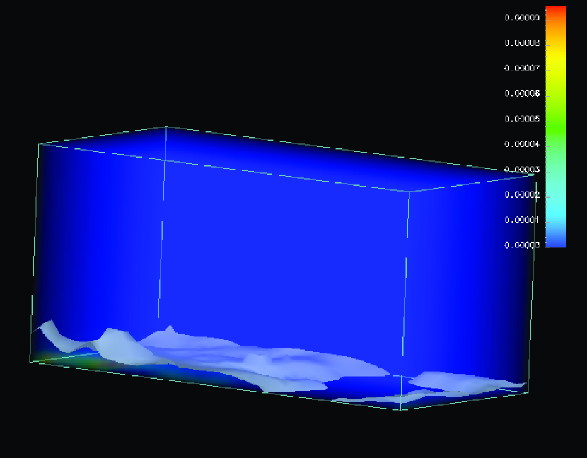
Figure 9: We display an iso-surface through the eigenvector density of the same chiral mode displayed in Fig 8. Here $s$ is the vertical direction, $t$ the left-right axis, and $z$ runs into the page. We show $(x,y)=(11,13)$ showing a uniformly well stuck region of this mode. Compared with the previous figure, this degree of binding is the more common case for this typical eigenvector, and one has to search spatially to find any localised incursion.

The localized low modes of $H_{W}$ thus play a role in providing conduits into the bulk for chiral symmetry breaking, causing corresponding localized spikes in the correlation function for $m_{\rm res}$. This is corroborated by the iso-surfaces (produced with the OpenDX package) of constant $H_{\rm DWF}$-eigenvector density (i.e. surfaces defined by $\Psi^{\dagger}(x,s)\Psi(x,s)={\rm constant}$) obtained in our simulation. Examples of this are shown in Figures 8 and 9, which represent lower dimensional views, at different spatial locations, of the same eigenvector. A movie, raster scanning $x$ and $y$ as a unified “movie-time”, can be obtained from .

Since the low modes of $H_{W}$ are scarce and very localized, it is to be expected that if we are in a region of parameter space where their contribution is the dominant contribution to chiral symmetry breaking, quantities such as $m_{\rm res}$ will display larger non-Gaussian tails (or “lumpiness”) than if the exponentially falling contribution from extended states is dominant. Thus, one should not be surprised by the need for very high statistics to achieve a convincing estimate for $m_{\rm res}$ in this region of parameter space.

VII Results for the residual mass

As discussed in Section IV, we calculate the residual mass from a ratio of correlation functions containing the axial Ward identity defect, $J^{b}_{5q}$, defined in Eq. 69:

$$R(t)=\frac{\sum_{\vec{y}}\langle J^{b}_{5q}(\vec{y},t)P^{b}(0)\rangle}{\sum_{\vec{y}}\langle J^{b}_{5}(\vec{y},t)P^{b}(0)\rangle}$$ (34)

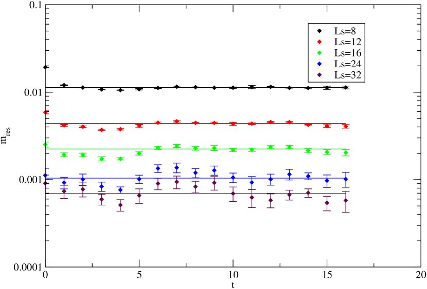
Figure 11: Residual mass fits for valence quarks with $m=0.04$ and $L_{s}=8,12,16,24,32$ on the DBW2 $\beta=0.72$ ensemble with sea quark masses $m_{ud}=m_{s}=0.04$, and for the sea quark $L_{s}=8$.

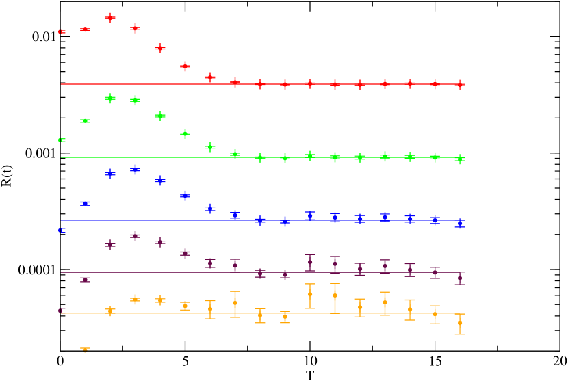
Figure 18: Residual mass fits for valence quarks with $m=0.04$ and $L_{s}=8,12,16,24,32$ on the Iwasaki $\beta=2.3$ ensemble with sea quark masses $m_{ud}=m_{s}=0.04$ and for the sea quark $L_{s}=8$.

where $b$ is a fixed flavor index, and $J^{b}_{5}(\vec{y},t)$ is the local 4-dimensional pseudoscalar density defined on the $s=0$ and $s=L_{s}-1$ walls. The operator $P^{b}(0)$ is either $J^{b}_{5}(\vec{y},t)$ or a spatially-smeared variant defined at $t=0$. The residual mass is determined from a constant fit to $R(t)$ over a range of times, $t$, that are sufficiently large that lattice artifacts should be absent. Recall that the ratio $R(t)$ should equal the residual mass provided that the numerator and denominator of Eq. 34 are dominated by physical states. There is not a requirement that only a specific lowest state contributes. For the calculations reported here this average is performed over the range $7\leq t\leq 16$. Figure 11 through Figure 18 contain plots of the fits of $R(t)$ to a constant. We use a combination of point, Coulomb gauge-fixed Wall and Coulomb gauge-fixed exponential sources on the various datasets listed in Table 2, and display the fitted values for $m_{\rm res}$ in Table 3 and Table 4 for the DBW2 and Iwasaki gauge actions respectively.

In order to conserve computer resources, we studied the dependence of $m_{\rm res}$ on $L_{s}$ by working with our fixed set of gauge configurations generated with $L_{s}=8$ but varying the “valence” value of $L_{s}$ that appears in the propagators used to compute the ratio in Eq. 34. The resulting $L_{s}$ dependence of the resulting $m_{\rm res}$ can be viewed as a (likely good) approximation to what would have been obtained if we also varied the $L_{s}$ appearing in the fermion determinant. This also can be viewed as a self-consistent study the properties of the 5-dimensional transfer matrix defined on gauge configurations generated with this fixed, $L_{s}=8$ fermion action.

Next we examine the degree to which Eq. 14 describes the dependence of $m_{\rm res}$ on $L_{s}$ in our simulations. Here we rewrite that equation in the form:

$$m_{\rm res}(L_{s})\simeq\left(c_{1}e^{-\lambda_{c}L_{s}}+c_{2}\right)\frac{1}{L_{s}}.$$ (35)

Recall that the first term is expected to come from extended states with eigenvalues $\lambda$ near the mobility edge: $\lambda_{c}\leq\lambda\leq\lambda_{c}+\frac{1}{L_{s}}$. This term is exponentially suppressed for large $L_{s}$ and thus can be easily reduced by increasing $L_{s}$. The second term arises from low-lying localized states with $0\leq\lambda\leq\frac{1}{L_{s}}$. Here $c_{2}$ is proportional to the density of near-zero modes, $\rho(0)$. We require a demonstrably non-zero mobility edge $\lambda_{c}$ for safe QCD simulations with chiral formulations. It is acceptable to have a significant non-exponential component in $m_{\rm res}$. However, the presence of such a term makes it difficult to significantly suppress chiral symmetry breaking effects by simply increasing $L_{s}$.

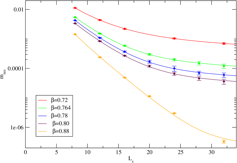
Figure 19: Valence $m_{\rm res}(L_{s})$ dependence of partially quenched DWF with the DBW2 gauge action as a function of $L_{s}$, using $L_{s}=8$ and the indicated $\beta$ values on a $16^{3}\times 32$ volume for the ensembles. The sea and valence quark masses are 0.04 throughout.

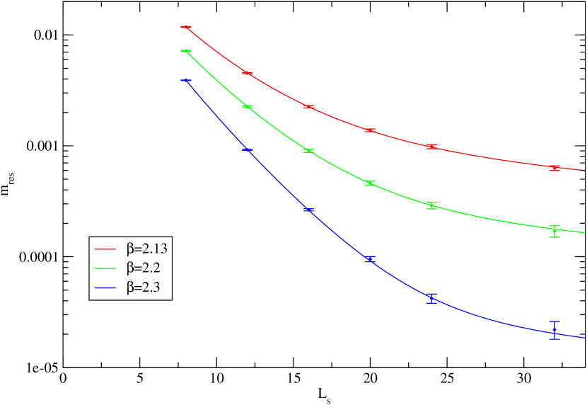
Figure 20: Valence $m_{\rm res}(L_{s})$ dependence of partially quenched DWF with the Iwasaki gauge action as a function of $L_{s}$, using $L_{s}=8$ and the indicated $\beta$ values on a $16^{3}\times 32$ volume for the ensembles. The sea and valence quark masses are 0.04 throughout.

We show fits to the functional form in Eq. 35 for degenerate three flavor ensembles at several gauge couplings for the Iwasaki and DBW2 gauge actions in Figures 19 and 20. The fitted parameters are listed in Table 5. While the exponent $\lambda_{c}$ increases only slowly, the parameter $c_{2}$ falls by orders of magnitude as the lattice spacing decreases. Interpolating between the values of lattice spacing given in these tables suggests the localized near-zero modes are suppressed more by the DBW2 than the Iwasaki gauge action. This behavior will be correlated with the rate of topology change discussed in the next section.

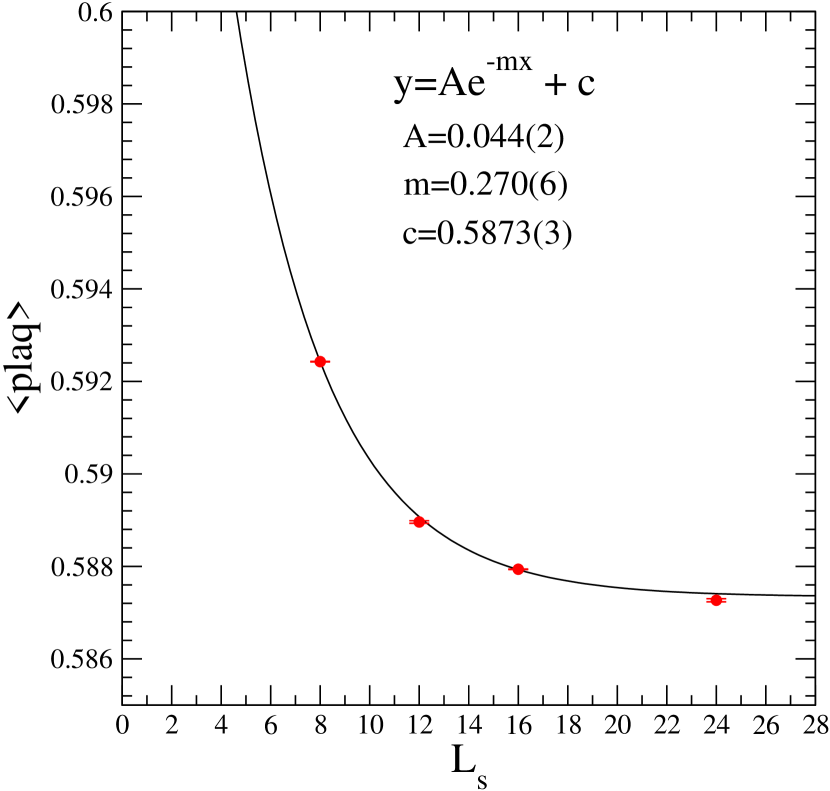
Figure 21: Dependence of the plaquette as a function of the dynamical $L_{s}$, obtained from low statistics runs. The dependence of this observable shows the expected $C+e^{-\alpha L_{s}}$ for an exponential approach to $L_{s}=\infty$, and thus demonstrates nicely the connection between finite $L_{s}$ DWF simulations and those with exactly chiral fermions.

We note that while the residual mass term may be incorporated in a renormalized quark mass, one should extrapolate to $L_{s}=\infty$ to remove the residual chiral symmetry breaking effects of the $c_{5}$ term in Eq. 3. However, even for finite $L_{s}$, such terms are expected to be very small compared with even the errors obtainable with non-perturbative improvement techniques for standard clover fermions, and thus can be treated as zero. Experience from clover fermions suggests that this level of error in the coefficient $c_{5}$ will certainly leave the results unmodified in practice, and that the unsuppressed $O(a^{2})$ errors will be dominant in a continuum extrapolation. Figure 21 displays the dependence of the simplest of observables, the plaquette, on $L_{s}$ for the sea quark content. It can be seen to be very weak (particularly for $L_{s}\geq 16$) and consistent with an exponential approach to the $L_{s}\to\infty$ limit, and is further evidence that all corrections to this limit are exponentially small.

VIII Localized Modes and Topology Change

Topology change, as defined by the index of an overlap operator will, be accompanied by a change of sign of a mode of $H_{W}(-M_{5})$ in the region $-2<-M_{5}<0$. There will be an instant $\tau=\tau_{0}(M_{5})$ in the molecular dynamics time at which $H_{W}(-M_{5})$ has an exact zero mode for any appropriate choice of $M_{5}$. Such a level crossing leaves the topological index of an overlap operator based on this kernel indefinite, depending on whether $-M_{5}$ is placed to the left or right of the level crossing, and it is reasonable to conjecture that low modes of $H_{W}(-M_{5})$ play a significant role in topology change in dynamical simulations with current algorithms.

In this section we shall present results for the topological charge time history in our ensembles, and consider the relationship between tunneling rates, the eigenmode spectrum, and details of the algorithm and action.

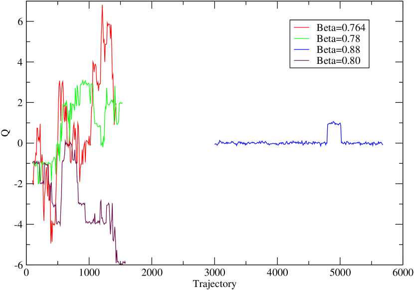
Figure 22: The Monte Carlo trajectory history for global topological charge with the DBW2 gauge action at couplings $\beta=0.72,0.764,0.78,0.8$. The $\beta=0.88$ history is offset by 3000 and displays a clear loss of topology tunneling. With a reasonable computational effort, a simulation with the current algorithm and these parameters would be practically non-ergodic.

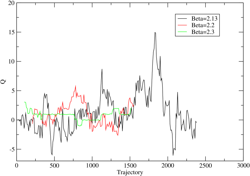
Figure 23: The Monte Carlo trajectory history for global topological charge with the Iwasaki gauge action at couplings $\beta=2.13,2.2,2.3$. The tunneling rate remains acceptable and leaves headroom for taking a continuum limit with acceptable topological sampling without any further algorithmic improvement.

In Figures 22 and 23 we display the topological charge time histories for all our datasets measured using the same $O(a^{2})$-improved definition of the topological charge density as in references Aoki et al. (2006); Antonio et al. (2006d), implemented using the Columbia Physics System. It is certainly the case that the tunneling rate is substantially lower in those datasets with lower spectral densities. These are also the configurations with the finest lattice spacings.

Sampling all topological sectors has proven problematic with RG improved gauge actions near the continuum limit even in the quenched approximation; some of the authors found previously that the DBW2 gauge action samples topological sectors rather poorly at $a^{-1}=3{\rm GeV}$ in the quenched case Aoki et al. (2004), and this loss of tunneling is likely driven by the gauge action. Going nearer to the continuum limit yields an increasing potential barrier between topological sectors, arising from the gauge action, which prevents topology change in those algorithms that either use a local update, or, even worse, Hamiltonian evolution to propose a next configuration.

Whenever the determinant of $H_{W}$ does not directly enter the probability weight, the spectral density of low modes of $H_{W}$ found for the resulting gauge configurations is principally determined by the degree of roughness admitted by the gauge action, likely corresponding to fluxon-like configurations Edwards et al. (1998); Berruto et al. (2000). We conjecture that for domain wall fermions at practical values for $L_{s}$ the tunneling rate is controlled by this low mode density.

VIII.1 Tunneling with dynamical overlap fermions

Additional problems have been seen with the introduction of exactly chiral fermions in dynamical simulations. Exact implementations of the overlap operator introduce a discontinuous step in the action when a low eigenvalue of $H_{W}$ changes sign (and hence when the topological index of the configuration changes). This infinitely narrow step in the action is guaranteed to be unresolved by numerical integration for any non-zero timestep, and leads to a high probability of rejection of the proposed configuration. The reflection/refraction algorithm Egri et al. (2006); Fodor et al. (2004) is one sensible, but expensive, response to this.

Another response has been to develop actions which suppress low modes of $H_{W}$ with pseudofermion determinant estimation Vranas (1999); Izubuchi and Dawson (2002); Fukaya et al. (2006), and so suppress topology change. While many hadronic quantities are not likely to be sensitive to global topology (especially in the limit of large volume), there remains a serious concern that a modification which suppresses the change of global topology may also interfere with the creation of a proper distribution of local topological fluctuations. In the language of instantons, one should demonstrate that such an algorithm leads to a physical density of instanton-anti-instanton pairs – a quantity that may be important for QCD even when the global topology is fixed. However, we have poor tools for knowing whether this globally non-ergodic algorithm is correctly sampling local topological fluctuations, given that we have thrown away our best diagnostic (and indeed the indicator that originally flagged the problem), i.e. global topology change.

So far with DWF we have obtained acceptable tunneling rates, and this is likely because the response to the lowest eigenvalues of the $\tanh$ approximation to the sign function, Eq. 1, is spread out at the level of our integration timestep. More specifically the determinant whose value is estimated contains a contribution $\tanh L_{s}\tanh^{-1}\lambda$, in place of ${\rm sgn}\lambda$, and the transition has a width of $O(\frac{1}{L_{s}})$. If we consider the low mode to be evolving in molecular dynamics time, with timestep $\delta\tau$ and at a rate $\dot{\lambda}$, then the molecular dynamics integral will be accurate provided

$$\delta\tau\ll\frac{1}{L_{s}\dot{\lambda}}.$$ (36)

There will be no practical impact on the tunneling rate from increasing $L_{s}$ while the condition Eq. 36 is held, and the problem may, in fact, never arise for any practical DWF simulation. In practice, the tunneling rate is determined by other effects, such as the low mode density determined by roughness admitted by the gauge action. We have also found a significant improvement in the tunneling rate, subsequent to this simulation arising from improving the quality of our stochastic estimate of the fermion force Allton et al. (2007), where the use of a single stochastic estimate for the ratio of Pauli-Villars and light mass determinants was found to allow increased molecular dynamics step size and to increase the tunneling rate.

This also suggests a third possible response to this problem that arises in simulations with better approximations to the overlap operator than our DWF simulations. That is to relax the approximation in the molecular dynamics evolution such that Eq. 36 is satisfied, while keeping the approximation accurate for the accept/reject step. This differential treatment of Metropolis and molecular dynamics steps is not possible with DWF simulations due to the fully five-dimensional pseudofermion fields, but it is possible for many approaches to the overlap operator.

IX Conclusion

When constrained to keep $L_{s}$ affordable, there is some degree of trade-off between the exactness of chirality and the thoroughness of topological sampling with domain wall fermions. Both are determined by the density of modes in the region where the $\tanh$ approximation is inaccurate, and this density is controlled by either the choice of the gauge action, or the inclusion of additional unphysical terms in the action.

One might pause for a moment to ponder where to compromise. Using computer precision, (e.g. single precision) as the standard for achieving chiral symmetry invokes computer technology rather than physics for an answer to this important question. The authors’ conclusion from this detailed study is that we should require adequate chirality, and by that we mean that the average symmetry breaking should not compromise the attractive simplification of electroweak current structure and off-shell $O(a)$ improvement for renormalization.

We have demonstrated in this paper that we can obtain $m_{\rm res}\simeq O(10^{-3})$ with both the DBW2 and Iwasaki gauge actions in the region of $a^{-1}\simeq 1.6{\rm GeV}$. We have observed that dynamical simulations with the DBW2 gauge action rapidly lose topological tunneling as $\beta$ is increased. In contrast, headroom is left for going to weaker coupling, while maintaining good topological sampling, with the Iwasaki gauge action. This approach is certainly at best a stay of execution, as topological tunneling will be lost on sufficiently fine lattices. These are inaccessible with our current computers and our conclusion is thus clear - the RBC and UKQCD collaborations are running Allton et al. (2007) dynamical domain wall fermions with the Iwasaki gauge action and $L_{s}\geq 16$. We started from $a^{-1}\simeq 1.6{\rm GeV}$ and thus we are able to maintain both excellent topological sampling and acceptable chiral symmetry violation.

Appendix A Domain wall fermion transfer matrix

Here we collect some useful formulae that describe the transfer matrix formalism as applied to domain wall fermions by Furman and Shamir Furman and Shamir (1995). While we do not present a derivation of these formulae, they follow reasonably directly from the results presented by Furman and Shamir, Narayanan and Neuberger Narayanan and Neuberger (1994) and Lüscher Luscher (1977).

We begin with the five-dimensional domain wall fermion Dirac operator defined in Eqs. 5, 6 and 7. (This definition of the domain wall fermion operator is consistent with our earlier papers, but differs by a hermitian conjugate from the original notation of Furman and Shamir.) We also identify two important 4-dimensional operators which play a central role in Lüscher’s original transfer matrix construction Luscher (1977):

$$B_{x,x^{\prime}} = (5-M_{5})\delta_{x,x^{\prime}}-\frac{1}{2}\sum_{\mu}\Bigl{[}\delta_{x+\mu,x^{\prime}}U_{x,\mu}+\delta_{x,x^{\prime}+\mu}U_{x^{\prime},\mu}^{\dagger}\Bigr{]}$$ (37)

$$C_{x,x^{\prime}} = \frac{1}{2}\sum_{\mu}\Bigl{[}\delta_{x+\mu,x^{\prime}}U_{x,\mu}-\delta_{x,x^{\prime}+\mu}U_{x^{\prime},\mu}^{\dagger}\Bigr{]}\sigma^{\mu}.$$ (38)

Here we have adopted a spinor basis in which $\gamma^{5}$ is diagonal. In this basis the $\gamma$ matrices can be written

$$\gamma^{\mu}=\left(\begin{array}[]{cc}0&\sigma^{\mu}\\ (\sigma^{\mu})^{\dagger}&0\end{array}\right)\quad\gamma^{5}=\left(\begin{array}[]{cc}1&0\\ 0&-1\end{array}\right)$$ (39)

and the four $2\times 2$ matrices $\sigma^{\mu}$ appearing in both Eqs. 38 and 39 are given by $\sigma^{\mu}=(i,\vec{\sigma})$, where $\vec{\sigma}$ represents the three standard Pauli matrices and $\frac{1}{2}(1\pm\gamma^{5})$ projects onto right-/left-handed states. Thus, the matrices $B$ and $C$ have a $2\times 2$-dimensional spin structure and appear directly in the matrix $D^{\parallel}_{x,x^{\prime}}(M_{5})$ of Eq. 6:

$$D^{\parallel}_{x,x^{\prime}}(M_{5}) = I-\left(\begin{array}[]{cc}B&C\\ C^{\dagger}&B\end{array}\right).$$ (42)

Next we need to introduce three pairs of related fermion fields. The first two pairs are the 5-dimensional Grassmann variables $\Psi_{x,s}$ and $\overline{\Psi}_{x,s}$ and the corresponding Fock-space operators $\hat{\psi}_{x}$ and $\hat{\overline{\psi}}_{x}$. The field operators $\hat{\psi}_{x}$ and $\hat{\overline{\psi}}_{x}$ can be written in terms of two-component field operators $\hat{c}_{x}$ and $\hat{d}_{x}$ and their hermitian conjugates:

$$\hat{\psi} = \left(\begin{array}[]{c}B^{-\frac{1}{2}}(\hat{d}^{\dagger})^{t}\\ B^{-\frac{1}{2}}\hat{c}\end{array}\right)$$ (45)

$$\hat{\overline{\psi}} = \left(\begin{array}[]{cc}-\hat{d}\,^{t}B^{-\frac{1}{2}},\quad\hat{c}^{\dagger}B^{-\frac{1}{2}}\end{array}\right).$$ (47)

Here the operators $\hat{c}$ and $\hat{d}$ both act on vectors in the Fock space and carry space-time, color and spinor indices. As Fock space operators, they can be thought of as $2^{12L^{3}L_{t}}$ dimensional square matrices if we are working with a $L^{3}\times L_{t}$ space-time lattice. We treat their space-time, color and spin indices as the index on a $6L^{3}L_{t}\times 1$ column vector. It is on this vector that the $6L^{3}L_{t}\times 6L^{3}L_{t}$ matrix $B^{-\frac{1}{2}}$ acts in Eqs. 45 and 47. We use the conventions that the hermitian conjugate, represented by the superscript $\dagger$ takes the hermitian conjugate of both the Fock-space operator and the space-time-flavor-spin matrix. The transpose, represented by the superscript $t$, acts only on the space-time-flavor-spin matrix.

Finally we introduce two further operators:

$$\hat{R}(\hat{c},\hat{d}) = \exp\Bigl{\{}\hat{d}^{t}(B^{-\frac{1}{2}}CB^{-\frac{1}{2}})\hat{c}\Bigr{\}}$$ (48)

$$\hat{W}(\hat{c}^{\dagger},\hat{d}^{\dagger},\hat{c},\hat{d}) = \exp\Bigl{\{}-\hat{c}^{\dagger}\ln(B)\hat{c}-\hat{d}^{\dagger}\ln(B)\hat{d}\Bigr{\}}.$$ (49)

Using these operators we can then connect the Feynman path integral, which provides the original definition of domain wall fermion lattice theory, with a Fock-space operator expression. For simplicity, we consider an example of the 5-dimensional fermion propagator, because a general fermionic Green’s function follows exactly the same pattern:

$$\int\prod_{x^{\prime},s^{\prime}}d[\Psi_{x^{\prime},s^{\prime}}]d[\overline{\Psi}_{x^{\prime},s^{\prime}}]e^{\overline{\Psi}D_{\rm DWF}\Psi}\;\Psi_{x_{1},s_{1}}\overline{\Psi}_{x_{2},s_{2}}$$ (51)

$$\hskip-144.54pt=\prod_{s=0}^{L_{s}-1}\Biggl{\{}\prod_{x}\int d\overline{\Psi}_{x,s}d\Psi_{x,s}\exp\Bigl{[}\overline{\Psi}^{R}_{s}\Psi^{L}_{s+1}+\overline{\Psi}^{L}_{s+1}\Psi^{R}_{s}-\overline{\Psi}^{L}_{s}B\Psi^{R}_{s}-\overline{\Psi}^{R}_{s}B\Psi^{L}_{s}$$

$$\hskip-108.405pt-\overline{\Psi}^{R}_{s}C^{\dagger}\Psi^{R}_{s}+\overline{\Psi}^{L}_{s}C\Psi^{L}_{s}\Bigr{]}\Biggr{\}}\Psi_{x_{1},s_{1}}\overline{\Psi}_{x_{2},s_{2}}$$

$$\hskip-144.54pt=(\det B)^{2L_{s}}\;\mbox{tr}\Biggl{\{}\Bigl{(}\hat{W}^{\frac{1}{2}}\hat{R}\hat{R}^{\dagger}\hat{W}^{\frac{1}{2}}\Bigr{)}^{s_{1}}\hat{W}^{\frac{1}{2}}\hat{R}\hat{\psi}_{x_{1}}\hat{R}^{\dagger}\hat{W}^{\frac{1}{2}}\Bigl{(}\hat{W}^{\frac{1}{2}}\hat{R}\hat{R}^{\dagger}\hat{W}^{\frac{1}{2}}\Bigr{)}^{s_{2}-s_{1}-1}$$

$$\hskip-108.405pt\hat{W}^{\frac{1}{2}}\hat{R}\hat{\overline{\psi}}_{x_{2}}\hat{R}^{\dagger}\hat{W}^{\frac{1}{2}}\Bigl{(}\hat{W}^{\frac{1}{2}}\hat{R}\hat{R}^{\dagger}\hat{W}^{\frac{1}{2}}\Bigr{)}^{L_{s}-s_{2}-1}{\cal{O}}(m_{f})\Biggr{\}}$$

where

$${\cal{O}}(m_{f})=\prod_{\alpha}\Bigl{\{}(\hat{c}_{\alpha}\hat{c}_{\alpha}^{\dagger}+m_{f}\hat{c}_{\alpha}^{\dagger}\hat{c}_{\alpha})(\hat{d}_{\alpha}\hat{d}_{\alpha}^{\dagger}+m_{f}\hat{d}_{\alpha}^{\dagger}\hat{d}_{\alpha})\Bigr{\}}$$ (52)

and $\alpha$ represents space-time, spin and color indices. While a complete derivation of the result in Eq. 51 is beyond the scope of this paper, one of the intermediate steps is shown in Eq. 51. In that equation the Grassmann fields $\Psi$ and $\overline{\Psi}$ have been expressed in terms of their chiral components according to:

$$\Psi=\left(\begin{array}[]{c}\Psi^{R}\\ \Psi^{L}\end{array}\right)\quad\overline{\Psi}=\left(\begin{array}[]{cc}\overline{\Psi}^{L}&\overline{\Psi}^{R}\end{array}\right).$$ (56)

A complete derivation of Eq. 51 can be constructed from Refs. Luscher (1977); Narayanan and Neuberger (1994); Furman and Shamir (1995). Note, the Grassmann fields $\Psi^{L}_{L_{s}}$ and $\overline{\Psi}^{L}_{L_{s}}$ appear in the integrand in Eq. 51 but are not among the variables of integration. Instead, these fields are to be evaluated as $-m_{f}$ times the corresponding fields at $s=0$: $-m_{f}\Psi^{L}_{s=0}$ and $-m_{f}\overline{\Psi}^{L}_{s=0}$, respectively.

Following Furman and Shamir, we identify the Fock-space transfer matrix $T$ as

$$T = (\det B)\hat{W}^{\frac{1}{2}}\hat{R}\hat{R}^{\dagger}\hat{W}^{\frac{1}{2}}=e^{-\hat{a}^{\dagger}H_{T}\hat{a}}$$ (57)

$$\mbox{where}\quad\hat{a} = \left(\begin{array}[]{c}(\hat{d}^{\dagger})^{t}\\ \hat{c}\end{array}\right),\quad\hat{a}^{\dagger}=\left(\begin{array}[]{cc}\hat{d}\,^{t},\quad\hat{c}^{\dagger}\end{array}\right)\quad\mbox{and}$$ (61)

$$e^{-H_{T}} = \left(\begin{array}[]{cc}B+CB^{-1}C^{\dagger}&CB^{-1}\\ B^{-1}C^{\dagger}&B^{-1}\end{array}\right).$$ (64)

The unusual arrangement of the operators $\hat{\psi}_{x_{1}}$ and $\hat{\overline{\psi}}_{x_{2}}^{\dagger}$ and two missing factors of $T$ in Eq. 51 can be understood if, following Furman and Shamir, we recognize that the upper component of $\hat{\psi}$ and the lower component of $\hat{\overline{\psi}}$ commute with $\hat{R}^{\dagger}$, while the lower component of $\hat{\psi}$ and the upper component of $\hat{\overline{\psi}}$ commute with $\hat{R}$. This allows the operators $\hat{\psi}$ and $\hat{\overline{\psi}}$ to be extracted from between the factors $\hat{W}^{\frac{1}{2}}\hat{R}$ and $\hat{R}^{\dagger}\hat{W}^{\frac{1}{2}}$, so that the two missing factors of $T$ can be assembled. (Note, the operators $\hat{\psi}$ and $\hat{\overline{\psi}}$ do not commute with the operator $\hat{W}^{\frac{1}{2}}$, but instead have the non-local factor of $B^{-\frac{1}{2}}$ appearing in Eqs. 45 and 47 removed by the proposed interchange).

We will demonstrate this re-arrangement of operators by working out two examples. In the first, we translate the expectation value $\langle\overline{q}(x)q(x)\rangle$ (the chiral condensate) into this transfer matrix language. Recall that the physical, 4-dimensional Grassmann fields are defined by:

$$q(x) = P_{L}\Psi_{x,0}+P_{R}\Psi_{x,L_{s}-1}$$ (65)

$$\overline{q}(x) = \overline{\Psi}_{x,0}P_{R}+\overline{\Psi}_{x,L_{s}-1}P_{L},$$ (66)

where we have used $P_{R/L}=(1\pm\gamma^{5})/2$. If these expressions are substituted into Eq. 51, we obtain:

$$\langle\overline{q}(x)q(x)\rangle = -(\det B)^{L_{s}}\mbox{tr}\Biggl{\{}\hat{W}^{\frac{1}{2}}\hat{R}(P_{L}\hat{\psi}_{x})_{\alpha}\hat{R}^{\dagger}\hat{W}^{\frac{1}{2}}$$

$$\quad\quad T^{L_{s}-2}\hat{W}^{\frac{1}{2}}\hat{R}(\hat{\overline{\psi}}_{x}P_{L})_{\alpha}\hat{R}^{\dagger}\hat{W}^{\frac{1}{2}}{\cal{O}}(m_{f})\Biggr{\}}$$

$$+ (\det B)^{L_{s}}\mbox{tr}\Biggl{\{}\hat{W}^{\frac{1}{2}}\hat{R}(\hat{\overline{\psi}}P_{R})_{\alpha}\hat{R}^{\dagger}\hat{W}^{\frac{1}{2}}$$

$$\quad\quad T^{L_{s}-2}\hat{W}^{\frac{1}{2}}\hat{R}(P_{R}\hat{\psi}_{x})_{\alpha}\hat{R}^{\dagger}\hat{W}^{\frac{1}{2}}{\cal{O}}(m_{f})\Biggr{\}}.$$

The final step involves commuting the $P_{L}\hat{\psi}$ and $\hat{\overline{\psi}}P_{R}$ past the factor $\hat{W}^{\frac{1}{2}}\hat{R}$ to stand on the far left. Similarly, the operators $P_{R}\hat{\psi}$ and $\hat{\overline{\psi}}P_{L}$ on the right side can be moved past the factor $\hat{R}^{\dagger}\hat{W}^{\frac{1}{2}}$ to stand directly to the left of the operator ${\cal{O}}(m_{f})$. The resulting expression can be written simply in terms of the operators $\hat{a}$ and $\hat{a}^{\dagger}$:

$$\langle\overline{q}(x)q(x)\rangle = -(\det B)^{L_{s}}\mbox{tr}\Biggl{\{}\Bigl{[}(P_{L}\hat{a}_{x})_{\alpha}T^{L_{s}}(\hat{a}^{\dagger}_{x}P_{L})_{\alpha}$$

$$\quad\quad\quad\quad+(\hat{a}_{x}^{\dagger}P_{R})_{\alpha}T^{L_{s}}(P_{R}\hat{a}_{x})_{\alpha}\Bigr{]}{\cal{O}}(m_{f})\Biggr{\}}.$$

As a second example, consider the Green’s function $\langle P_{L}q(x)\;J^{b}_{5q}(z)\;\overline{q}(y)P_{L}\rangle$ containing the midpoint operator $J^{a}_{5q}$ that occurs in the divergence of the 5-dimensional flavor non-singlet axial current introduced by Furman and Shamir Furman and Shamir (1995):

$$J^{b}_{5q}(x)=-\overline{\Psi}(x,L_{s}/2-1)P_{L}t^{b}\Psi(x,L_{s}/2)+\overline{\Psi}(x,L_{s}/2)P_{R}t^{b}\Psi(x,L_{s}/2-1).$$ (69)

Here $b$ is a flavor index and $t^{b}$ is a flavor generator.

Using Eq. 51 for this product of four Grassmann fields we find:

$$\langle P_{L}q(x)\;J^{b}_{5q}(z)\;\overline{q}(y)P_{L}\rangle = -(\det B)^{L_{s}}\mbox{tr}\Biggl{\{}\hat{W}^{\frac{1}{2}}\hat{R}(P_{L}\hat{\psi}_{x})\hat{R}^{\dagger}\hat{W}^{\frac{1}{2}}T^{L_{s}/s-2}$$

$$\Bigl{[}-\hat{W}^{\frac{1}{2}}\hat{R}(\hat{\overline{\psi}}_{z}P_{L}t^{b})_{\alpha}\hat{R}^{\dagger}\hat{W}^{\frac{1}{2}}\hat{W}^{\frac{1}{2}}\hat{R}(P_{L}\hat{\psi}_{z})_{\alpha}\hat{R}^{\dagger}\hat{W}^{\frac{1}{2}}$$

$$\quad-\hat{W}^{\frac{1}{2}}\hat{R}(t^{b}P_{R}\hat{\psi}_{z})_{\alpha}\hat{R}^{\dagger}\hat{W}^{\frac{1}{2}}\hat{W}^{\frac{1}{2}}\hat{R}(\hat{\overline{\psi}}_{z}P_{R})_{\alpha}\hat{R}^{\dagger}\hat{W}^{\frac{1}{2}}\Bigr{]}$$

$$\quad\quad T^{L_{s}/s-2}\hat{W}^{\frac{1}{2}}\hat{R}(\hat{\overline{\psi}}_{y}P_{R})\hat{R}^{\dagger}\hat{W}^{\frac{1}{2}}{\cal{O}}(m_{f})\Biggr{\}}.$$

Performing the same operator manipulations as used to obtain Eq. A we find:

$$\langle P_{L}q(x)\;J^{b}_{5q}(z)\;\overline{q}(y)P_{L}\rangle = (\det B)^{L_{s}}\mbox{tr}\Bigl{\{}P_{L}\hat{a}_{x}T^{\frac{L_{s}}{2}}\hat{a}^{\dagger}_{z}t^{b}\hat{a}_{z}T^{\frac{L_{s}}{2}}\hat{a}^{\dagger}_{y}P_{L}{\cal{O}}(m_{f})\Bigl{\}}.$$ (71)

Here the unit displacement in $s$ between the two factors in $J^{a}_{5q}$ has disappeared leaving a very symmetrical expression. The missing $\gamma^{5}$ matrix, which one would expect in an axial matrix element, has its origins in the minus sign that is present in Eq. 47 but absent in Eq. 61. This factor could be restored if we introduced $\hat{\overline{a}}_{x}=\hat{a}_{x}^{\dagger}\gamma^{5}$, a 5-dimensional analogue of the role played by $\gamma^{0}$ in the standard treatment of the 4-dimensional Dirac operator.

As a final topic for this appendix, we will examine the effects of the matrix $T^{L_{s}}$ in Eq. A. Again following Furman and Shamir, we introduce the eigenvectors and eigenvalues of the operator $H_{T}$ defined in Eq. 64:

$$H_{T}\phi^{+}_{k^{+}}=E^{+}_{k^{+}}\phi^{+}_{k^{+}}\quad 1\leq k^{+}\leq N^{+}$$ (72)

$$H_{T}\phi^{-}_{k^{-}}=-E^{-}_{k^{-}}\phi^{-}_{k^{-}}\quad 1\leq k^{-}\leq N^{-}$$ (73)

where $E^{\mp}_{n}\geq 0$, and write the operator $\hat{a}_{x}$ in terms of this basis, filling the Dirac sea in the usual way :

$$\hat{a}_{x}=\sum_{k+=1}^{N^{+}}\phi^{+}_{k^{+}}(x)\;\hat{o}_{k}+\sum_{k^{-}=1}^{N^{-}}\phi^{-}_{k^{-}}(x)\;\hat{p}_{k^{-}}^{\dagger}.$$ (74)

Let $|0_{H}\rangle$ be the Fock space state $|0_{H}\rangle$ which is the eigenstate of $T$ with the largest eigenvalue. This state obeys:

$$\hat{o}_{k^{+}}|0_{H}\rangle=\hat{p}_{k^{-}}|0_{H}\rangle=0$$ (75)

for all $k^{+}$ and $k^{-}$ and

$$T|0_{H}\rangle=\lambda_{\rm max}|0_{H}\rangle=\exp\left\{\sum_{k^{-}=1}^{N^{-}}E^{-}_{k^{-}}\right\}|0_{H}\rangle.$$ (76)

Finally we define the normalized operator $\hat{T}=T/\lambda_{\rm max}$ making unity the largest eigenvalue of $\hat{T}$ and $|0_{H}\rangle$ the corresponding eigenstate. The matrix $\hat{T}$ can be written:

$$\hat{T} = T/\lambda_{\rm max}=\exp\left\{-\hat{a}^{\dagger}H\hat{a}\right\}/\lambda_{\rm max}$$ (77)

$$= \exp\left\{-\sum_{k^{+}=1}^{N^{+}}E^{+}_{k^{+}}\hat{o}_{k^{+}}^{\dagger}\hat{o}_{k^{+}}+\sum_{k^{-}=1}^{N^{-}}E^{-}_{k^{-}}\hat{p}_{k^{-}}\hat{p}_{k^{-}}^{\dagger}\right\}/\lambda_{\rm max}$$ (78)

$$= \exp\left\{-\sum_{k^{+}=1}^{N^{+}}E^{+}_{k^{+}}\hat{o}_{k^{+}}^{\dagger}\hat{o}_{k^{+}}-\sum_{k^{-}=1}^{N^{-}}E^{-}_{k^{-}}\hat{p}_{k^{-}}^{\dagger}\hat{p}_{k^{-}}\right\}.$$ (79)

Thus, in the limit of large $L_{s}$, $\hat{T}^{L_{s}}$ becomes the projection operator onto the state $|0_{H}\rangle$, separating the right and left operators in an equation such as Eq. A into two separate factors, linked by the operator ${\cal{O}}(m_{f})$. If we further take the limit $m_{f}=0$ and define a surface vacuum state $|0_{S}\rangle$, which is annihilated by the operators $\hat{c}_{x}$ and $\hat{d}_{x}$,

$$\hat{c}_{x}|0_{S}\rangle=\hat{d}_{x}|0_{S}\rangle=0,$$ (80)

then the operator ${\cal{O}}(m_{f}=0)$, given in Eq. 52, reduces to the projection operator $|0_{S}\rangle\langle 0_{S}|$ and the left- and right-handed sectors become completely independent matrix elements between $|0_{S}\rangle$ and $|0_{H}\rangle$.

This can be summarized by evaluating a general Green’s function depending on the 4-dimensional fields $q$ and $\overline{q}$. This is most easily done if the fermion fields in the original Green’s function are ordered with the left-handed chiral fields ($P_{L}q$ and $\overline{q}P_{R}$) on the left and the right-handed chiral fields ($P_{R}q$ and $\overline{q}P_{L}$) on the right:

$$\frac{1}{(\det B\;\lambda_{\rm max})^{L_{s}}}\left\langle{\cal O}_{L}[P_{L}q,\overline{q}P_{R}]\;{\cal O}_{R}[P_{R}q,\overline{q}P_{L}]\right\rangle_{L_{s}}\hskip-180.67499pt$$ (84)

$$=\frac{1}{(\lambda_{\rm max})^{L_{s}}}\;{\rm tr}\left\{{\cal O}_{L}[P_{L}\hat{a},-\hat{a}^{\dagger}P_{R}]T^{L_{s}}{\cal O}_{R}[P_{R}\hat{a},\hat{a}^{\dagger}P_{L}]{\cal{O}}(m_{f})\right\}$$

$$\hskip-7.22743pt\mathrel{\mathop{\rightarrow}_{L_{s}\to\infty}}{\rm tr}\left\{{\cal O}_{L}[P_{L}\hat{a},-\hat{a}^{\dagger}P_{R}]|0_{H}\rangle\langle 0_{H}|{\cal O}_{R}[P_{R}\hat{a},\hat{a}^{\dagger}P_{L}]{\cal{O}}(m_{f})\right\}$$

$$\hskip-7.22743pt\mathrel{\mathop{\rightarrow}_{m_{f}\to 0}}\langle 0_{S}|{\cal O}_{L}[P_{L}\hat{a},-\hat{a}^{\dagger}P_{R}]|0_{H}\rangle\langle 0_{H}|{\cal O}_{R}[P_{R}\hat{a},\hat{a}^{\dagger}P_{L}]|0_{S}\rangle,$$

where the quantities ${\cal O}_{L}$ and ${\cal O}_{R}$ are two ordered polynomials in their two arguments.

Corrections to the limit $L_{s}\to\infty$ can be written by including eigenvectors of $\hat{T}$ with smaller eigenvalues. Such corrections can be easily obtained from Eq. 79:

$$\hat{T}^{L_{s}}\approx|0_{H}\rangle\langle 0_{H}|+\sum_{k^{+}=1}^{N^{+}}e^{-E^{+}_{k^{+}}L_{s}}\hat{o}_{k^{+}}^{\dagger}|0_{H}\rangle\langle 0_{H}|\hat{o}_{k^{+}}+\sum_{k^{-}=1}^{N^{-}}e^{-E^{-}_{k^{-}}L_{s}}\hat{p}_{k^{-}}^{\dagger}|0_{H}\rangle\langle 0_{H}|\hat{p}_{k^{-}}+\ldots.$$ (85)

Table 1: Ensembles used in this study. We also document the trajectories used for $m_{\rm res}$ measurements, using every tenth trajectory in the given range. The trajectory length was $\tau=0.5$ units of MD time. All ensembles used three degenerate DWF flavors of mass $m=0.04$, and $M_{5}=1.8$.

Gauge Action	$\beta$	Algorithm	Trajectories
DBW2	0.72	R	800-1500
DBW2	0.764	R	800-1500
DBW2	0.78	R	1000-1600
DBW2	0.80	R	900-1800
DBW2	0.88	R	1000-3000
Iwasaki	2.13	RHMC	1500-2400
Iwasaki	2.2	RHMC	800-1500
Iwasaki	2.3	RHMC	800-1500

Table 2: Correlation functions generated for valence quarks with different extents of the fifth dimension on each of our $L_{s}=8$ dynamical ensembles. The valence and sea quark masses were $m_{ud}=m_{s}=0.04$. We denote point source correlators as “P”, wall source correlators as “W”, and exponentially smeared correlators as “S”.

Dataset	$L_{s}=8$	$L_{s}=12$	$L_{s}=16$	$L_{s}=20$	$L_{s}=24$	$L_{s}=28$	$L_{s}=32$
Iwasaki $\beta=2.13$	S	S	S	S	S	-	S
Iwasaki $\beta=2.2$	W,P	P	P	P	P	-	P
Iwasaki $\beta=2.3$	W,P	P	P	P	P	-	P
DBW2 $\beta=0.72$	W	W	W	-	W	-	W
DBW2 $\beta=0.764$	W	P	P	P	P	P	P
DBW2 $\beta=0.78$	W	W,P	W,P	W,P	W,P	P	P
DBW2 $\beta=0.80$	W	P	P	P	P	P	P
DBW2 $\beta=0.88$	P	W,P	W,P	W,P	W,P	-	W,P

Table 3: Fitted residual mass values for valence quarks with different extents of the fifth dimension for the DBW2 gauge action on each of our $L_{s}=8$ dynamical ensembles. The valence and sea quark masses were $m_{ud}=m_{s}=0.04$.

Dataset	$L_{s}=8$	$L_{s}=12$	$L_{s}=16$	$L_{s}=20$	$L_{s}=24$	$L_{s}=28$	$L_{s}=32$
$\beta=0.72$	$1.13(1)\times 10^{-2}$	$4.4(1)\times 10^{-3}$	$2.2(1)\times 10^{-3}$	-	$1.04(5)\times 10^{-3}$	-	$7.0(5)\times 10^{-4}$
$\beta=0.764$	$5.46(4)\times 10^{-3}$	$1.53(3)\times 10^{-3}$	$5.9(2)\times 10^{-4}$	$3.0(2)\times 10^{-4}$	$2.0(2)\times 10^{-4}$	$1.5(2)\times 10^{-4}$	$1.2(2)\times 10^{-4}$
$\beta=0.78$	$4.28(3)\times 10^{-3}$	$1.09(2)\times 10^{-3}$	$3.7(2)\times 10^{-4}$	$1.7(1)\times 10^{-4}$	$1.0(2)\times 10^{-4}$	$7(1)\times 10^{-5}$	$6(1)\times 10^{-5}$
$\beta=0.80$	$3.39(2)\times 10^{-3}$	$8.4(2)\times 10^{-4}$	$2.7(1)\times 10^{-4}$	$1.2(1)\times 10^{-4}$	$6.6(8)\times 10^{-5}$	$4.6(7)\times 10^{-5}$	$3.6(7)\times 10^{-5}$
$\beta=0.88$	$1.441(4)\times 10^{-3}$	$2.40(2)\times 10^{-4}$	$4.87(6)\times 10^{-5}$	$1.14(3)\times 10^{-5}$	$3.0(1)\times 10^{-6}$	-	$3.3(4)\times 10^{-7}$

Table 4: Fitted residual mass values for valence quarks with different extents of the fifth dimension for the Iwasaki gauge action on each of our $L_{s}=8$ dynamical ensembles. The valence and sea quark masses were $m_{ud}=m_{s}=0.04$.

Dataset	$L_{s}=8$	$L_{s}=12$	$L_{s}=16$	$L_{s}=20$	$L_{s}=24$	$L_{s}=32$
$\beta=2.13$	$1.18(1)\times 10^{-2}$	$4.53(5)\times 10^{-3}$	$2.25(5)\times 10^{-3}$	$1.38(4)\times 10^{-3}$	$9.8(4)\times 10^{-4}$	$6.3(3)\times 10^{-4}$
$\beta=2.2$	$7.19(6)\times 10^{-3}$	$2.25(4)\times 10^{-3}$	$9.0(3)\times 10^{-4}$	$4.6(2)\times 10^{-4}$	$2.9(2)\times 10^{-4}$	$1.7(2)\times 10^{-4}$
$\beta=2.3$	$3.90(2)\times 10^{-3}$	$9.2(1)\times 10^{-4}$	$2.65(6)\times 10^{-4}$	$9.5(5)\times 10^{-5}$	$4.2(4)\times 10^{-5}$	$2.2(4)\times 10^{-5}$

Table 5: Fit parameters to the dependence of $m_{\rm res}$ on $L_{s}$ for the Iwasaki and DBW2 gauge actions. We also give the lattice spacing obtained from the static potential Hashimoto et al. (2006); Antonio et al. (2006d) on the dynamical background for $m_{ud}=m_{s}=0.04$ without chiral extrapolation. This differs from the lattice spacing defined in the chiral limit presented in Antonio et al. (2006d), and we only provide the lattice spacings here for illustration.

Action	$\beta$	$c_{1}$	$\lambda_{c}$	$c_{2}$	$a^{-1}$(GeV)
Iwasaki	2.13	0.344(6)	0.191(2)	0.0198(3)	1.62(2)
Iwasaki	2.2	0.301(4)	0.219(2)	0.0054(1)	1.89(2)
Iwasaki	2.3	0.262(3)	0.268(2)	0.0006(1)	2.26(7)
DBW2	0.72	0.342(10)	0.201(4)	0.0220(4)	1.40(4)
DBW2	0.764	0.298(6)	0.252(3)	0.0040(1)	1.74(3)
DBW2	0.78	0.267(5)	0.264(2)	0.00188(7)	1.82(2)
DBW2	0.80	0.216(5)	0.265(3)	0.00120(5)	1.98(4)
DBW2	0.88	0.171(7)	0.338(5)	1.0(5)$\times 10^{-5}$	-

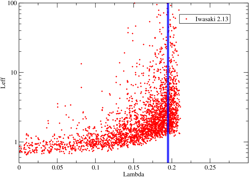
Figure 7: Microscopic view of the mobility edge based on a scatter plot of maximal localization lengths of individual low eigenmodes of $H_{W}$. We overlay the $H_{T}$ mobility edge $\lambda_{c}$ from fits to the model for $m_{\rm res}$, Eq 35 and find good agreement with our diverging localisation length for the Iwasaki gauge action at $\beta=2.13$.

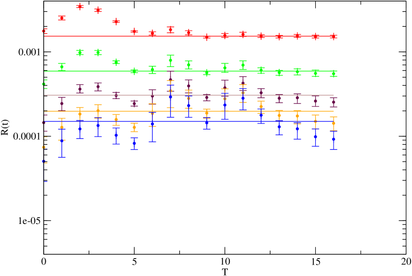
Figure 12: Residual mass fits for valence quarks with $m=0.04$ and $L_{s}=8,12,16,24,32$ on the DBW2 $\beta=0.764$ ensemble with sea quark masses $m_{ud}=m_{s}=0.04$ and for the sea quark $L_{s}=8$.

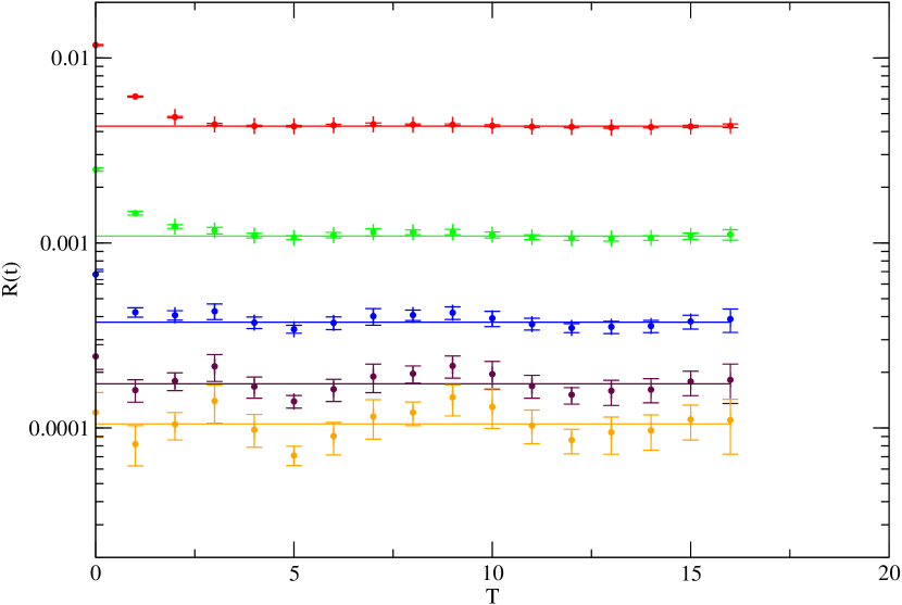
Figure 13: Residual mass fits for valence quarks with $m=0.04$ and $L_{s}=8,12,16,24,32$ on the DBW2 $\beta=0.78$ ensemble with sea quark masses $m_{ud}=m_{s}=0.04$ and for the sea quark $L_{s}=8$.

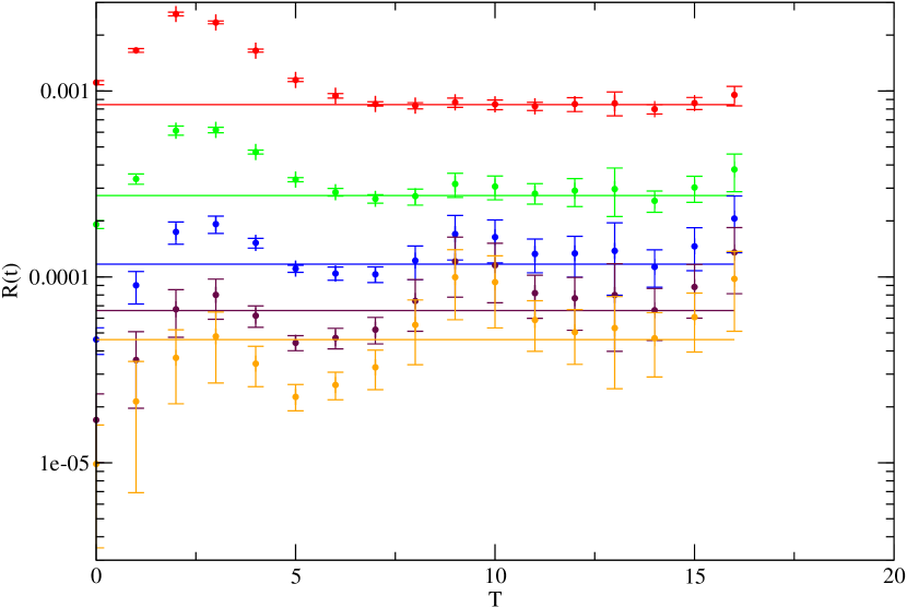
Figure 14: Residual mass fits for valence quarks with $m=0.04$ and $L_{s}=8,12,16,24,32$ on the DBW2 $\beta=0.80$ ensemble with sea quark masses $m_{ud}=m_{s}=0.04$ and for the sea quark $L_{s}=8$.

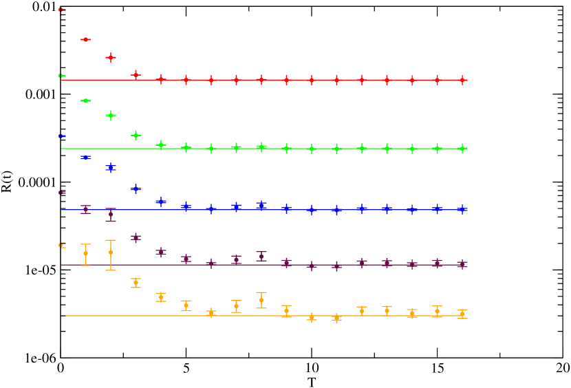
Figure 15: Residual mass fits for valence quarks with $m=0.04$ and $L_{s}=8,12,16,24,32$ on the DBW2 $\beta=0.88$ ensemble with sea quark masses $m_{ud}=m_{s}=0.04$ and for the sea quark $L_{s}=8$.

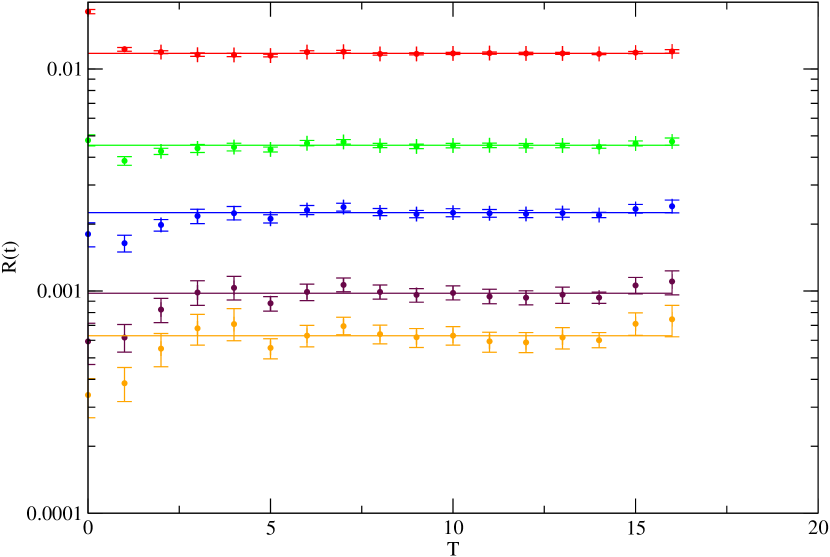
Figure 16: Residual mass fits for valence quarks with $m=0.04$ and $L_{s}=8,12,16,24,32$ on the Iwasaki $\beta=2.13$ ensemble with sea quark masses $m_{ud}=m_{s}=0.04$ and for the sea quark $L_{s}=8$.

Figure 17: Residual mass fits for valence quarks with $m=0.04$ and $L_{s}=8,12,16,24,32$ on the Iwasaki $\beta=2.2$ ensemble with sea quark masses $m_{ud}=m_{s}=0.04$ and for the sea quark $L_{s}=8$.

References

- Kaplan (1992) D. B. Kaplan, Phys. Lett. B288, 342 (1992), eprint hep-lat/9206013.
- Neuberger (1998a) H. Neuberger, Phys. Lett. B417, 141 (1998a), eprint hep-lat/9707022.
- Furman and Shamir (1995) V. Furman and Y. Shamir, Nucl. Phys. B439, 54 (1995), eprint hep-lat/9405004.
- Aoki (1984) S. Aoki, Phys. Rev. D30, 2653 (1984).
- Clark and Kennedy (2004) M. A. Clark and A. D. Kennedy, Nucl. Phys. Proc. Suppl. 129, 850 (2004), eprint hep-lat/0309084.
- Clark et al. (2005) M. A. Clark, A. D. Kennedy, and Z. Sroczynski, Nucl. Phys. Proc. Suppl. 140, 835 (2005), eprint hep-lat/0409133.
- Boyle et al. (2005) P. Boyle et al., Nucl. Phys. Proc. Suppl. 140, 169 (2005).
- Boyle et al. (2002) P. A. Boyle et al., Nucl. Phys. Proc. Suppl. 106, 177 (2002), eprint hep-lat/0110124.
- Boyle et al. (2003) P. A. Boyle, C. Jung, and T. Wettig (QCDOC), ECONF C0303241, THIT003 (2003), eprint hep-lat/0306023.
- Aoki (1986a) S. Aoki, Phys. Rev. D33, 2399 (1986a).
- Aoki (1986b) S. Aoki, Phys. Rev. Lett. 57, 3136 (1986b).
- Aoki and Taniguchi (2002) S. Aoki and Y. Taniguchi, Phys. Rev. D65, 074502 (2002), eprint hep-lat/0109022.
- Aoki et al. (2002) S. Aoki et al. (CP-PACS), Nucl. Phys. Proc. Suppl. 106, 718 (2002), eprint hep-lat/0110126.
- Golterman and Shamir (2003) M. Golterman and Y. Shamir, Phys. Rev. D68, 074501 (2003), eprint hep-lat/0306002.
- Golterman et al. (2005a) M. Golterman, Y. Shamir, and B. Svetitsky, Phys. Rev. D71, 071502 (2005a), eprint hep-lat/0407021.
- Golterman et al. (2005b) M. Golterman, Y. Shamir, and B. Svetitsky, Phys. Rev. D72, 034501 (2005b), eprint hep-lat/0503037.
- Svetitsky et al. (2006) B. Svetitsky, Y. Shamir, and M. Golterman, PoS LAT2005, 129 (2006), eprint hep-lat/0508015.
- Neuberger (1998b) H. Neuberger, Phys. Rev. D57, 5417 (1998b), eprint hep-lat/9710089.
- Kikukawa and Noguchi (1999) Y. Kikukawa and T. Noguchi (1999), eprint hep-lat/9902022.
- Hernandez et al. (1999) P. Hernandez, K. Jansen, and M. Luscher, Nucl. Phys. B552, 363 (1999), eprint hep-lat/9808010.
- Borici (2000) A. Borici, Nucl. Phys. Proc. Suppl. 83, 771 (2000), eprint hep-lat/9909057.
- Edwards and Heller (2001) R. G. Edwards and U. M. Heller, Phys. Rev. D63, 094505 (2001), eprint hep-lat/0005002.
- Borici (1999) A. Borici (1999), eprint hep-lat/9912040.
- Antonio et al. (2006a) D. J. Antonio et al. (RBC and UKQCD), PoS LAT2005, 141 (2006a).
- Yamada et al. (2006) N. Yamada et al. (JLQCD) (2006), eprint hep-lat/0609073.
- Christ (2006) N. Christ (RBC and UKQCD), PoS LAT2005, 345 (2006).
- Shamir (1993) Y. Shamir, Nucl. Phys. B406, 90 (1993), eprint hep-lat/9303005.
- Narayanan and Neuberger (1995) R. Narayanan and H. Neuberger, Nucl. Phys. B443, 305 (1995), eprint hep-th/9411108.
- Blum et al. (2004) T. Blum et al., Phys. Rev. D69, 074502 (2004), eprint hep-lat/0007038.
- Aoki et al. (2004) Y. Aoki et al., Phys. Rev. D69, 074504 (2004), eprint hep-lat/0211023.
- Aoki et al. (2005) Y. Aoki et al., Phys. Rev. D72, 114505 (2005), eprint hep-lat/0411006.
- Iwasaki (1985) Y. Iwasaki, Nucl. Phys. B258, 141 (1985).
- Iwasaki and Yoshie (1984) Y. Iwasaki and T. Yoshie, Phys. Lett. B143, 449 (1984).
- Takaishi (1996) T. Takaishi, Phys. Rev. D54, 1050 (1996).
- de Forcrand et al. (2000) P. de Forcrand et al. (QCD-TARO), Nucl. Phys. B577, 263 (2000), eprint hep-lat/9911033.
- Gottlieb et al. (1987) S. A. Gottlieb, W. Liu, D. Toussaint, R. L. Renken, and R. L. Sugar, Phys. Rev. D35, 2531 (1987).
- Clark and Kennedy (2007a) M. A. Clark and A. D. Kennedy, Phys. Rev. Lett. 98, 051601 (2007a), eprint hep-lat/0608015.
- Clark and Kennedy (2007b) M. A. Clark and A. D. Kennedy, Phys. Rev. D75, 011502 (2007b), eprint hep-lat/0610047.
- Antonio et al. (2006b) D. J. Antonio et al. (UKQCD), PoS LAT2005, 080 (2006b), eprint hep-lat/0512009.
- Antonio et al. (2006c) D. J. Antonio et al. (RBC), PoS LAT2005, 098 (2006c), eprint hep-lat/0511011.
- Antonio et al. (2006d) D. J. Antonio et al. (2006d), eprint hep-lat/0612005.
- Edwards and Joo (2005) R. G. Edwards and B. Joo (SciDAC), Nucl. Phys. Proc. Suppl. 140, 832 (2005), eprint hep-lat/0409003.
- (43) P. Boyle, http://www.ph.ed.ac.uk/~paboyle/bagel/Bagel.html.
- Antonio et al. (2006e) D. J. Antonio et al. (RBC and UKQCD), PoS LAT2005, 135 (2006e).
- Sharpe and Singleton (1998) S. R. Sharpe and J. Singleton, Robert L., Phys. Rev. D58, 074501 (1998), eprint hep-lat/9804028.
- Aoki et al. (2006) Y. Aoki et al., Phys. Rev. D73, 094507 (2006), eprint hep-lat/0508011.
- Berruto et al. (2000) F. Berruto, R. Narayanan, and H. Neuberger, Phys. Lett. B489, 243 (2000), eprint hep-lat/0006030.
- Edwards et al. (1998) R. G. Edwards, U. M. Heller, and R. Narayanan, Nucl. Phys. B535, 403 (1998), eprint hep-lat/9802016.
- Egri et al. (2006) G. I. Egri, Z. Fodor, S. D. Katz, and K. K. Szabo, JHEP 01, 049 (2006), eprint hep-lat/0510117.
- Fodor et al. (2004) Z. Fodor, S. D. Katz, and K. K. Szabo, JHEP 08, 003 (2004), eprint hep-lat/0311010.
- Vranas (1999) P. M. Vranas (1999), eprint hep-lat/0001006.
- Izubuchi and Dawson (2002) T. Izubuchi and C. Dawson (RBC), Nucl. Phys. Proc. Suppl. 106, 748 (2002).
- Fukaya et al. (2006) H. Fukaya et al. (JLQCD), Phys. Rev. D74, 094505 (2006), eprint hep-lat/0607020.
- Allton et al. (2007) C. Allton et al. (2007), eprint hep-lat/0701013.
- Narayanan and Neuberger (1994) R. Narayanan and H. Neuberger, Nucl. Phys. B412, 574 (1994), eprint hep-lat/9307006.
- Luscher (1977) M. Luscher, Commun. Math. Phys. 54, 283 (1977).
- Hashimoto et al. (2006) K. Hashimoto, T. Izubuchi, and J. Noaki (RBC-UKQCD), PoS LAT2005, 093 (2006), eprint hep-lat/0510079.