Spitzer observations of a 24$\micron$ shadow: Bok Globule CB190

Abstract

We present Spitzer observations of the dark globule CB190 (L771). We observe a roughly circular 24$\micron$ shadow with a $70\arcsec$ radius. The extinction profile of this shadow matches the profile derived from 2MASS photometry at the outer edges of the globule and reaches a maximum of $\sim\!32$ visual magnitudes at the center. The corresponding mass of CB190 is $\sim\!10$ $\hbox{M}_{\odot}$. Our ¹²CO and ¹³CO J = 2-1 data over a 10$\arcmin\times$10$\arcmin$ region centered on the shadow show a temperature $\sim\!10$ K. The thermal continuum indicates a similar temperature for the dust. The molecular data also show evidence of freezeout onto dust grains. We estimate a distance to CB190 of 400 pc using the spectroscopic parallax of a star associated with the globule. Bonnor-Ebert fits to the density profile, in conjunction with this distance, yield $\xi_{max}=7.2$, indicating that CB$190$ may be unstable. The high temperature (56 K) of the best fit Bonnor-Ebert model is in contradiction with the CO and thermal continuum data, leading to the conclusion that the thermal pressure is not enough to prevent free-fall collapse. We also find that the turbulence in the cloud is inadequate to support it. However, the cloud may be supported by the magnetic field, if this field is at the average level for dark globules. Since the magnetic field will eventually leak out through ambipolar diffusion, it is likely that CB$190$ is collapsing or in a late pre-collapse stage.

1. Introduction

Cold cloud cores, where star formation begins, represent the stage in early stellar evolution after the formation of molecular clouds and before the formation of Class 0 objects. Their emission is inaccessible at shorter wavelengths, such as the near infrared and visual bands, due to low temperatures, very high gas densities, and associated large amounts of dust. Because cold cloud cores can best be observed at sub-millimeter and far-infrared wavelengths, these spectral regions are essential to developing an understanding of the first steps toward star-formation (see, e.g., Bacmann et al., 2000; Kirk et al., 2007). The wavelength range accessible to the Spitzer Space Telescope, 3.6 $\micron$ to 160 $\micron$, is ideally suited to observe cold, dense regions.

CB$190$ (L771) is an example of one such dark globule and is classified in the Lynds catalog as having an opacity of 6 (Lynds, 1962), i.e., very high. Clemens & Barvainis (1988) study this object as part of an optically selected survey of small molecular clouds. They find that it appears optically isolated, is somewhat asymmetric ($a/b\sim 2.5$) and has some bright rims of reflection and H$\alpha$. CB$190$ is $\sim\!5\arcmin$ across, and has an estimated distance of 400 pc (Neckel et al., 1980).

We present Spitzer maps of CB$190$. In particular, we highlight the observation of this globule in absorption at 24 $\micron$. We combine these data with SCUBA observations at 850 $\micron$. We have obtained complementary Heinrich Hertz Telescope (HHT) ¹²CO and ¹³CO J=2-1 on the fly (OTF) maps of this globule and have used the HHT and Green Bank Telescope (GBT) to measure high resolution line profiles for ¹²CO, ¹³CO, NH₃, CCS, C₃S, and HC₅N. We report C¹⁸O and DCO⁺ measurements with the Caltech Submillimeter Observatory (CSO). We discuss the issue of stability and possible support mechanisms in some detail; however, we cannot say conclusively if CB$190$ is in equilibrium. In § 2 we describe the observations and data processing. In § 3 we present our main analysis of CB$190$: we derive an optical depth and an extinction profile for the 24 $\micron$ shadow using a technique presented for the first time in this work. We also discuss two sources associated with CB$190$ and derive a distance estimate. In § 4 we compare various mass estimates of this object. In § 5 we describe our Bonnor-Ebert fitting method and discuss possible support mechanisms for CB$190$. Finally, in § 6 we summarize our main conclusions. All positions are given in the J2000 system.

2. Observations and processing

2.1. Spitzer data

Object CB$190$ (L$771$), centered at about RA = $19^{h}20^{m}48^{s}$, Dec = $+23^{o}29\arcmin 45\arcsec$, was observed with the MIPS instrument (Rieke et al., 2004) at $24$ $\micron$, $70$ $\micron$ and $160$ $\micron$, Spitzer program ID $53$ (P.I. G. Rieke). The observations were carried out in scan map mode. Figure 1 shows these data, along with the Digital Sky Survey (DSS) red plate image of the globule.

The 24 $\micron$ data were reduced using version 3.06 of the MIPS Data Analysis Tool (DAT; Gordon et al. 2005). In addition to the standard processing, several other additional steps have been applied: 1) correcting for variable offsets among the four readouts; 2) applying a scan-mirror position-dependent flat field; 3) applying a scan-mirror position-independent flat field to remove long term gain changes due to previous saturating sources; and 4) background subtraction. For the last two steps, masks of any bright sources and also of the region of interest were used to ensure that the two corrections were unbiased. The background subtraction was performed by fitting a low order polynomial to each scan leg of the masked data and subtracting the resulting fit. This procedure removes the contribution of zodiacal and other background light as well as small transients seen after a boost frame.

The 70 $\micron$ and 160 $\micron$ data were also reduced using the DAT (Gordon et al. 2005). After completing the standard reduction processing, an additional correction was performed to remove the long term drift in the Ge:Ga detectors. The correction was determined by fitting a low order polynomial to the masked version of the entire dataset for each pixel. By masking bright sources as well as the region of interest we ensure that the masked-version fits are unbiased. The resulting fits for each pixel were subtracted to remove the long term drift as well as any background light.

CB$190$ was observed with the IRAC instrument (Fazio et al., 2004) at $3.6$, $4.5$, $5.8$ and $8.0$ $\micron$, program ID $94$  (P.I. C. Lawrence), see fig. 2. Standard packages were used to reduce the data, and the mosaicked frames were generated with the MOPEX software package. The data were taken in high dynamic range mode; the $30$ second exposure time was divided into a $1.0$s “short” frame and a $26.8$ s “long” frame at each position. Each observation was repeated $5$ times, yielding an effective long-frame exposure time of $134$ s. SExtractor (Bertin & Arnouts, 1996) was used for both source extraction and photometry. The photometry was cross-checked with PhotVis version $1.1$, an IDL GUI-based implementation of DAOPHOT (Gutermuth et al., 2004). We found good agreement between the two sets of photometry.

2.2. ¹²CO and ¹³CO data

The CB$190$ region was mapped in the J=2-1 transitions of ¹²CO and ¹³CO with the 10-m diameter HHT on Mt. Graham, Arizona on 2005 June 9. The receiver was a dual polarization SIS mixer system operating in double-sideband mode with a 4 - 6 GHz IF band. The ¹²CO J=2-1 line at 230.538 GHz was placed in the upper sideband and the ¹³CO J=2-1 line at 220.399 GHz in the lower sideband, with a small offset in frequency to ensure that the two lines were adequately separated in the IF band. The spectrometers, one for each of the two polarizations, were filter banks with 1024 channels of 1 MHz width and separation. At the observing frequencies, the spectral resolution was 1.3 km s^-1 and the angular resolution of the telescope was 32$\arcsec$ (FWHM).

A $10\arcmin\times 10\arcmin$ field centered at RA = $19^{h}20^{m}49.5^{s}$, Dec = $+23^{o}29\arcmin 57\arcsec$ was mapped with on-the-fly (OTF) scanning in RA at $10\arcsec$ sec^-1, with row spacing of $10\arcsec$ in declination, over a total of 60 rows. This field was observed twice, each time requiring about 100 minutes of elapsed time. System temperatures were calibrated by the standard ambient temperature load method (Kutner & Ulich, 1981) after every other row of the map grid. Atmospheric conditions were clear and stable, and the system temperatures were nearly constant at $T_{sys}=450$ K (SSB).

Data for each polarization and CO isotopomer were processed with the CLASS reduction package (from the University of Grenoble Astrophysics Group), by removing a linear baseline and convolving the data to a square grid with $16\arcsec$ grid spacing (equal to one-half the telescope beamwidth). The intensity scales for the two polarizations were determined from observations of DR21(OH) made just before the OTF maps. The gridded spectral data cubes were processed with the Miriad software package (Sault et al., 1995) for further analysis. The two polarizations were averaged, yielding images with rms noise per pixel and per velocity channel of 0.15 K-T${}_{A}^{*}$ for both the ¹²CO and ¹³CO transitions.

The linewidths were narrow, so that 70% of the flux in the ¹²CO J=2-1 line was in a single 1 MHz spectrometer channel, while essentially all the flux of the ¹³CO line was in a single channel. We can therefore set an upper limit of $\sim\!1.3$ km s^-1 on the linewidth for the emission lines, but have little or no kinematic information from the maps, other than the LSR velocity, which is 11.0 km s^-1, in agreement with Clemens & Barvainis (1988). In figure 3 we show two maps of the integrated ¹²CO and ¹³CO J=2-1 lines, summed over the 2 spectrometer channels with detectable emission. Furthermore, in figure 4, we show the ¹³CO J=2-1 contours overlayed on the 24 $\micron$ image; the spatial coincidence between the two is evident.

To better constrain the CO line properties, we observed the core of the molecular cloud with high velocity resolution on 2006 June 21 with the HHT. The position observed was at RA = $19^{h}20^{m}46.4^{s}$, Dec = $+23^{o}29\arcmin 45\farcs 6$, which is the peak of the ¹²CO intensity map (fig. 3). Both the ¹²CO and ¹³CO J=2-1 transitions were observed for 15 minutes each. The high resolution ¹²CO and ¹³CO spectra are shown in fig. 5. The ¹²CO line is slightly asymmetric, with a peak beam-averaged brightness temperature of 7.65 K, and a velocity width (FWHM) of 1.22 km s^-1. The ¹³CO line is narrower, with a FWHM of 0.97 km s^-1, and has a peak intensity of 2.96 K. The ¹²CO/¹³CO intensity ratio at the line peak is therefore $\sim\!2.6$; if the isotopic ratio [¹²CO/¹³CO] = 50, the optical depth of the ¹³CO line at the peak is $\sim\!0.5$, and the line is optically thin. While values for [¹²CO/¹³CO] in the range of 50 to 70 are reasonable, see e.g., Milam et al. (2005), changing the isotopic ratio will not significantly affect our calculated optical depth. We can then compute an integrated CO column density assuming the CO rotational levels are in LTE. Following Rohlfs & Wilson (2004), the peak ¹²CO line brightness temperature implies a CO excitation temperature of 12.6 K. Assuming this applies to both isotopomers, the integrated ¹³CO J=2-1 line intensity gives an integrated column density of N(¹³CO)$=2\times 10^{15}$ cm^-2 at the cloud peak, and N(¹²CO) $=9\times 10^{16}$ cm^-2. If the [CO/H₂] abundance ratio were $1.5\times 10^{-4}$, typical of molecular clouds, the column density of H₂ would be N(H₂) $=6\times 10^{20}$ cm^-2. A standard gas to dust ratio and extinction law would then imply $A_{V}$ = 0.7 mag through the cloud core. This very low implied extinction is clearly incompatible with the observed large extinction evident in the POSS image from which the L771 dark cloud was identified. This discrepancy suggests that the CO molecule is substantially depleted by freeze-out onto dust grains in the core of the cloud, as has been seen in many other molecular cloud cores (e.g., Tafalla et al. 2002). We confirm this conclusion in § 4.3.

2.3. Observations of other molecular lines

Observations of CB190 were performed with the 105 meter Green Bank Telescope on September 20, 2006. Five spectral lines were observed simultaneously in dual polarization: NH₃ (1,1) and (2,2), CCS $N_{J}=1_{2}-2_{1}$, C₃S $J=4-3$, and HC₅N $J=9-8$. The correlator was set up with 6.1 kHz resolution and 8 spectral windows ($4RR$ and $4LL$ polarizations) with a 50 MHz bandpass. The peak ¹³CO position was observed for 20 minutes of ON-source integration time while frequency switching with a frequency throw of 4.15 MHz. The atmospheric optical depth at 1.3 cm was calibrated using the weather model of Ron Maddalena (private communication, 2006). The average opacity was $\tau_{1.3}=0.095\pm 0.010$ during the CB190 observations. The main beam efficiency was determined from observations of the quasars 3C286 and 3C48 and was $\eta_{mb}=0.75\pm 0.04$. The observations were reduced using standard GBTIDL script for frequency-switched observations, calibrated using the latest K-band receiver T_cal for each polarization, and corrected for atmospheric opacity and the main beam efficiency.

Michael M. Dunham (private communication, 2006) provided C¹⁸O J = 2 - 1 and DCO⁺ J = 3 - 2 observations obtained with the Caltech Submillimeter Observatory. The observations were performed in position-switching mode with the 50 MHz AOS backend. The main beam efficiency was measured to be 0.74 during the observing run. C¹⁸O J = 2 - 1 was detected toward the 24 $\mu$m shadow peak position, but DCO⁺ was not detected to a 3 $\sigma$ rms of 0.4  K.

The molecular line emission detected toward CB190 is striking in its lack of diversity. Only CO isotopomers and NH₃ have been detected to date. The early-time molecules CCS, C₃S, and HC₅N were not detected with the GBT to a 25 mK (T${}_{R}^{*}$) baseline rms while the deuteration tracer, DCO⁺ was not detected in the CSO observations. The NH₃ (1,1) line is weak, with a peak T${}_{R}^{*}=200\pm 23$ mK and a narrow linewidth of $\Delta v=0.47\pm 0.08$ km s^-1. Since the main line is a blend of many hyperfine lines, the actual linewidth is smaller. The optical depth is low enough that the satellite lines are barely detected at the $3\sigma$ level. Assuming an excitation temperature of 10 K and optically thin emission, the column density of NH₃ is $N=5.4^{+0.6}_{-0.4}\times 10^{12}$ cm^-2. This column density is two orders of magnitude below the median column density in the NH₃ survey of Jijina et al. (1999) and is six times lower than their weakest detection. A modest 20 minute integration time on the GBT can probe very low column densities of NH₃. Unfortunately, the (2,2) line was also not detected to the 23 mK baseline rms level; therefore, we cannot independently determine the kinetic temperature of the gas. The extremely weak NH₃ emission and DCO⁺ non-detection may indicate that CB190 is a relatively young core. In contrast, there is evidence that CO is depleted indicating that the core is not a nascent dense core. A more extensive and sensitive search for molecular line emission should be attempted toward CB190 to characterize its chemistry.

2.4. 2MASS Data

We used the 2MASS All-Sky Point Source Catalog (PSC) (Skrutskie et al., 2006) photometry. We quote the default J, H, and K-band photometry in this work, labeled j_-m, h_-m, and k_-m in the 2MASS table header. The magnitudes are derived over a 4$\arcsec$ radius aperture. We use the combined, or total, photometric uncertainties for the default magnitudes, labeled j_-msigcom, h_-msigcom, and k_-msigcom in the 2MASS table header.

2.5. SCUBA Data

We include in this work the Visser et al. (2002) reduced 850$\micron$ SCUBA map of CB$190$ (Claire Chandler, private communication, 2006). This map was convolved with a 32$\arcsec$ FWHM Gaussian beam and is shown in figure 6 as contours overlayed on the 160 $\micron$ data. The spatial agreement between the two wavelengths is very good. We note, however, that the southern edge of the cloud may be artificially sharpened at 850$\micron$ due to the position angle of chopping during the scan map. Figure 7 shows photometry for the 70 $\micron$, 160 $\micron$ and 850 $\micron$ observations, measured with a 48$\arcsec$ radius aperture centered on the 24 $\micron$ shadow coordinates. The observed ratio of the long wavelength fluxes is $f_{\nu}[160\micron]/f_{\nu}[850\micron]=3.1$. With this ratio we fit for a cloud temperature using the model

$$f_{\nu}\propto\nu^{\beta}B_{\nu}(T).$$ (1)

We fix the value of $\beta$ at 1.5 and 2.0, a reasonable range of values for dust emissivity (Whittet, 2003), and derive best-fit model temperatures of 12.0 K and 10.4 K, respectively. These two models are plotted in figure 7. The 160 $\micron$ flux is well detected, with a signal to noise ratio $\sim\!20$, indicating that these temperatures are robust. However, to test the models conservatively, we recalculate model temperatures allowing for 20% errors in our photometry. We do not find significant variation in the derived temperatures. We note that the lack of a detection at 70 $\micron$ mildly favors the colder temperature of 10.4 K. The $3\sigma$ upper limit to the flux density at 70 $\micron$ is $\sim\!16$ mJy while the predicted values are 17 mJy for the $\beta=1.5$, T = 12 K model, and 6 mJy for the $\beta=2.0$, T = 10.4 K model.

Visser et al. (2002) find that the CB$190$ SCUBA 450 $\micron$ emission is spatially offset from the 850 $\micron$ data for reasons that are not understood. Because we find good spatial agreement between the 850 $\micron$ data and the 160 $\micron$ image (see fig. 6), we do not use the 450 $\micron$ map. The need for deep sub-mm or mm observations of this region is highlighted by the fact that both of the SCUBA maps have low S/N, suffer from ambiguities in the spatial extent of the cloud due to the chopping position, and have poorly understood spatial disagreements between the 850 $\micron$ and 450 $\micron$ observations.

2.6. Optical Spectrum

We have obtained optical spectra of three stars: HD344204 (star 1 in figure 4), HD1608, and Vega. These spectra cover the optical range, from 3615Å to 6900Å with an effective resolution of $\Delta\lambda$ = 9Å, and were observed in July 2006 at the Steward Observatory Bok 2.3m telescope at Kitt Peak using the Boller and Chivens Spectrograph with a 400/mm grating in first order. They were processed with standard IRAF data reduction packages. These data are shown in figure 8 and discussed in SS 3.1 and 3.2.

3. Analysis

3.1. Two associated stellar sources

There are two bright sources in the 24$\micron$ image that are likely associated with CB$190$. The first, labeled source 1 in fig. 4, is a bright point source, just to the north of the 24 $\micron$ shadow, with a large amount of diffuse emission. This star is HD344204 (IRAS 19186+2325), and is located at RA = $19^{h}20^{m}47^{s}$, Dec = $23^{o}31\arcmin 40.6\arcsec$. The second star, labeled source 2 in fig. 4, is spatially coincident with a small peak in the ¹³CO emission, and is located at RA = $19^{h}20^{m}57^{s}$, Dec = $23^{o}31\arcmin 37.6\arcsec$. The broad-band SEDs of these two sources are plotted in fig. 9, and include 2MASS (Skrutskie et al., 2006) J, H, and K data (see § 2.3), IRAC [3.6 $\micron$], [4.5 $\micron$], [5.8 $\micron$], and [8.0 $\micron$] data, and MIPS 24 $\micron$ fluxes. Although star 1 appears to be indistinguishable from the surrounding diffuse emission in figure 4, this is only due to the scale used to display the image. To measure the flux of the star while avoiding contamination from the surrounding diffuse emission we use a very small photometry aperture radius, $6.23\arcsec$, and sky annulus, $6.23\arcsec$ to $7.47\arcsec$. We derive an aperture correction of 2.1 to this flux using an isolated point source, measured with the same aperture geometry as that listed above. We compare this result to the flux derived using a $13\arcsec$ aperture, a $20\arcsec$ to $32\arcsec$ sky annulus, and the 24 $\micron$ aperture correction recommended by the Spitzer Science Center. For comparison fig. 9 also indicates the 24 $\micron$ flux of Star 1 measured with a large aperture with radius $=30\arcsec$ and an inner and outer sky annulus radius $=34\arcsec$ and $38\arcsec$ respectively, meant to include all the light from the diffuse emission surrounding the source.

In fig. 9 we also show the broad-band SED of source 2. The IRAC colors are ([3.6 $\micron$]-[4.5 $\micron$]) = 0.5 mag, and ([5.8 $\micron$]-[8.0 $\micron$]) = 1.1 mag. The models by Whitney et al. (2003) suggest that these colors are consistent with those of a late Class 0 source.

3.2. The Distance

To understand the nature of the CB$190$ 24 $\micron$ shadow one must measure its physical properties, such as mass and size; to do so one needs an accurate distance. While star counts are commonly used to estimate distances to nearby clouds, in the case of CB$190$ this method is not reliable due to the small number of foreground sources. Another distance estimator is the LSR velocity relation. However, this method is not reliable for nearby objects whose motions are still locally dominated, as is the case of CB$190$. Neckel et al. (1980) estimate the distance to this cloud to be $\sim\!400$ pc using the discontinuity in A_V with distance. Dame & Thaddeus (1985) argue that this distance is consistent with the narrow line width they measure and therefore reject the other plausible distance to this cloud, that of the Vul OB1 association at 2.3 kpc, noting that this longer distance would imply a much larger mass and line width.

We can obtain a rough estimate of the distance using the colors of source 2 (see fig. 9) and the Whitney et al. (2003) models. Their color-magnitude ([5.8 $\micron$]-[8.0 $\micron$]) vs. [3.6 $\micron$] relation for a face-on late Class 0 source, with [3.6 $\micron]\sim 8$ mags, yields a distance $\sim\!700$ pc. If we assume a model with the same ([5.8 $\micron$]-[8.0 $\micron$]) color but which is slightly more inclined, with a [3.6 $\micron]\sim 9.7$ mags, we obtain a distance $\sim\!330$ pc. These distance estimates are highly speculative, as the uncertainty in the magnitudes makes the observed colors marginally consistent with later-type models. Furthermore, these models are relatively untested.

In this context, i.e., determining a distance to CB$190$, source 1 (see fig. 4) draws attention for two reasons. This star has a large amount of diffuse emission at 24 and 70 $\micron$. It is also coincident with the truncation of the ¹³CO emission on the northern edge of CB$190$. Based on these two facts we conclude that source 1 is very likely to be associated with the cloud. Our spectrum of source 1 shows it to be a B7 star, based on the strong Balmer absorption lines and HeI features that are evident in fig. 8. Assuming this is a main-sequence star, its distance is $\sim\!400$ pc, and if it is a giant (luminosity class III) its distance is $\sim\!600$ pc. The broad feature observed in the spectrum of this source near 5700Å may be due to the reddening curve. As a matter of historical interest, A. J. Cannon classified this star as B9. In the following analysis, where it is relevant, we assume a distance of $400$ pc.

3.3. Extinction law analysis

We have used the IRAC and 2MASS data to probe the extinction law in CB$190$. These data are used to generate the color-color plots shown in fig. 10. We calculate the errors in these colors by adding the respective IRAC and 2MASS K-band errors in quadrature; the median values of these errors are plotted in the lower right corner of fig. 10. To analyze the colors, we compare the best-fit reddening vector to those measured by Indebetouw et al. (2005). We consider stars to be reddened if their colors are more than $2\sigma$ away from the mean colors of the ensemble. These reddened stars are indicated in fig. 10 as open boxes. We then fit the slope of the reddening vector, including both x- and y-errors, using the IDL routine fitexy.pro (Press et al., 1992). We also include the median value of the unreddened stars and assign it zero error. The resulting reddening vector slope is shown in fig. 10 as a solid black line. Because this slope agrees reasonably well with the Indebetouw et al. (2005) extinction vectors, we conclude that the dust found in CB$190$ is not anomalous and that we are justified in using a “standard” reddening law to determine the dust properties in this globule. The agreement with the Indebetouw et al. (2005) extinction is not surprising because, as was shown in Harris et al. (1978) and Rieke & Lebofsky (1985), there is generically almost no difference in the infrared extinction in dense clouds even though the visual bands may deviate significantly from their low-density values. We note that we exclude source 2, discussed in § 3.1, from this analysis for two reasons: first, because it has a very large 24 $\micron$ excess, and second, because its broad-band SED is consistent with the colors of a proto-star, being too red to be simply due to a foreground dust screen and a normal star (see fig. 9).

3.4. The 24 $\micron$ shadow: Optical depth and column density profile

The 24 $\micron$ image shows a shadow, or depression in the emission, centered at RA = $19^{h}20^{m}48^{s}$, Dec = $+23^{o}29\arcmin 45\arcsec$ (see fig. 1), coincident with the location of the dark cloud CB$190$ (L771; e.g., Clemens & Barvainis, 1988; Visser et al., 2002). This shadow, about 70$\arcsec$ in radius, is coincident with the peak in the ¹²CO and ¹³CO maps (see figs. 3 and 4), the 160 $\micron$ emission (see fig. 1), and the SCUBA emission (see fig. 6). We do not observe a shadow at 70 and 160 $\micron$. In fact, at 70 $\micron$ the cloud is at best only marginally detected in emission and may be dominated by the light from source 1 just to the north of the 24 $\micron$ shadow. The shadow at 24 $\mu$m is a result of the cold and dense material in CB$190$ blocking the background radiation.

In the following derivation of the density profile we correct for the large-scale foreground emission at 24 $\micron$ (see $f_{DC}$ and discussion below). This large-scale component is likely to be composed mainly of zodiacal light; if we underestimate it we will effectively wash out the shadow signal and therefore underestimate its optical depth profile, density profile, and mass. Conversely, if we overestimate the large-scale background level, we will also overestimate the optical depth profile. Keeping this in mind, we estimate the zodiacal contribution by using the darkest parts of the image. Therefore, strictly speaking, we are deriving an upper limit to the optical depth profile. This approach is conservative because it allows us to derive a robust profile consistently and independently, without having to use other data to set the normalization of the density profile. While it is possible that the emission varies on shorter scales and, more specifically, emission from CB$190$ fills in the 24 $\micron$ shadow, we consider this to be unlikely due to the fact that the shadow is not detected at 70 $\micron$. It is not plausible that CB$190$ would be emitting significantly at 24 $\micron$ while remaining undetected at the longer wavelength. In the following discussion we describe the method used to derive the optical depth and extinction profile for the 24 $\micron$ shadow.

First, we estimate the overall large-scale uniform background level in the image, $f_{DC}$. We do so using two dark regions in the image, free from sources, indicated by boxes in fig. 1, one to the North-East and one to the South-West of the shadow, each one about 50$\arcsec$ on a side. We use the first percentile flux value in these boxes, $f_{DC}=-5.732$ mJy arcsec^-2, as a lower limit on the overall uniform level in the image. We use this background level to set the true image zero level by subtracting it from the original image. Then we mask out all bright sources in the image by clipping all pixels with values $3\sigma$ above the mean. Finally, we use this background-subtracted and bright-source masked image to derive an optical-depth and extinction profile. For completeness, we estimate the error in $f_{DC}$ by simulating the pixel distribution in the two dark regions. We estimate $\sigma_{DC}$ by simulating $n_{pix}=3362$ pixel values drawn from a normal density with mean and standard deviation equal to those measured in the two regions and storing the first percentile pixel value. We repeat $10^{4}$ times, and calculate the standard deviation in the simulated $f_{DC}$ of $\sigma_{DC}=0.083$ mJy arcsec^-2.

We proceed by dividing the shadow into regions of nested (concentric and adjacent) annuli $2.5\arcsec$ in width, the inner-most region being a circle with a radius of $2.5\arcsec$. These regions are centered on the darkest part of the shadow, which is also roughly coincident with the peak in the ¹³CO emission. We measure the average flux per pixel in each region out to a radius of $\sim\!100\arcsec$, chosen to be big enough to allow for a reasonable estimate of the background immediately adjacent to the shadow. We show the derived radial profile in fig. 11. Based on this profile, we set the boundary of the shadow to be at a radius of $67\farcs 5$ (marked in fig. 11 with a solid line) where there is a flattening in the derived profile. We estimate the background flux by averaging the values of the annuli outside $70\arcsec$ and within $100\arcsec$. This background value is marked in figure 11 with a dashed line.

We use this profile to calculate the optical depth $\tau_{24}$ of the shadow. In a given annulus $\tau_{24}$ is given by $\tau_{24}=-\ln(I/I_{0})$, where $I_{0}$ is the background level and $I$ is the shadow flux. The calculated value of $\tau_{24}$ varies from $\sim\!1.5$ at the center to about 0.02 at a radius of $67\farcs 5$. The average mass column density in each annulus is then given by

$$\Sigma=\frac{\tau_{24}}{\kappa_{abs,24}}f,$$ (2)

where $f(=100)$ is the gas-to-dust ratio, and $\kappa_{abs,24}$ is the absorption cross-section per mass of dust. In this work we use the value of $\kappa_{abs,24}=5.283\times 10^{2}$ cm² gm^-1 calculated by Draine (2003a, b) from his $R_{V}=5.5$ model. The choice of a model with a high $R_{V}$ value relative to the diffuse ISM is intended to account for some of the grain-growth effects likely to be taking place in CB$190$, as evidenced by the depletion indicated by our ¹²CO and ¹³CO data. This column density profile can be converted to an extinction profile using the relation $N(H_{2})/$A${}_{V}=1.87\times 10^{21}$ atoms cm^-2 mag^-1 (Bohlin et al., 1978), where we assume that all of the hydrogen is in molecular form. We use a value of $R_{V}=3.1$, appropriate for the diffuse ISM where this relation was measured, to convert from $E(B-V)$ to $A_{V}$. The corresponding extinction is given by

$$A_{\rm V}=\frac{\Sigma}{1.87\times 10^{21}\,{\rm cm}^{-2}\,{\rm mag}^{-1}\mu_{\rm H_{2}}m_{\rm H}},$$ (3)

where $\mu_{\rm H_{2}}$ is the effective molecular weight per hydrogen molecule. The molecular weight per hydrogen molecule is related to the mass fraction of hydrogen, $\mathcal{M({\rm H})}/\mathcal{M}$ (where $\mathcal{M}=\mathcal{M({\rm H})}+\mathcal{M({\rm He})}+\mathcal{M({\rm Z})}$), by

$$\mu_{\rm H_{2}}=\frac{\mathcal{M}}{m_{\rm H}N(\rm H_{2})}=\frac{2\mathcal{M}}{m_{\rm H}N(\rm H)}=\frac{2\mathcal{M}}{\mathcal{M({\rm H})}}.$$ (4)

For a cosmic hydrogen mass fraction $\mathcal{M({\rm H})}/\mathcal{M}=0.71$, $\mu_{\rm H_{2}}=2.8$ (Jens Kauffmann - private communication, 2006). We consider two sources of uncertainty in the column density profile for the 24 $\micron$ shadow: the DC-background error and the uncertainty in our assumed dust model, $\kappa_{abs,24}$. We measure an error in the DC-background level of $\sigma_{DC}=0.083$ mJy arcsec^-2 (described above). We then calculate the corresponding uncertainty in A_V by propagating $\sigma_{DC}$ through the equation for $\tau_{24}$ and scaling appropriately. We estimate the dust model uncertainty to be half of the difference in $\kappa_{abs,24}$ between the Weingartner & Draine (2001) $R_{V}=3.1$ model and the $R_{V}=5.5$ model. To obtain an estimate of the total uncertainty in $A_{V}$, we add these two components and a $10\%$ systematic error floor in quadrature.

The column density profile and corresponding errors are shown in figure 12 along with individual 2MASS point-source extinction estimates. We use 2MASS sources with data quality flags better than, and including, “UBB”, and include “C” quality measurements in a bandpass when the other two filters are “B” quality or better. Sources with upper limits in two or more bands are rejected. This selection ensures that we include the maximum number of quality extinction measurements while not biasing the object selection towards stars with lower amounts of reddening. The reddening of the accepted sources is measured using the $(J-K)$ color and the Rieke & Lebofsky (1985) extinction law: $A_{V}=E(J-K)/0.17$. The “intrinsic” $(J-K)_{0}=1.34$ color of the stars is measured in the 70$\arcsec$ to 100 $\arcsec$ annulus centered on the shadow, to isolate the effects of the globule from that of nearby diffuse dust. We reject sources between 0$\arcsec$ and 70$\arcsec$ with $E(J-K)$ values lower than $-0.37$, the 1-$\sigma$ value for the scatter in the sources between 70$\arcsec$ and 100$\arcsec$. This 1-$\sigma$ range is marked in figure 12 with two dotted lines. Two sources fulfill this criterion, located at r $\sim\!25\arcsec,67\arcsec$ from the center. We reject one other source with an A${}_{V}\sim 3$ located at $r\sim 9\arcsec$ on the basis that it is likely to be a foreground object. We calculate a probability of 1.4% of finding three foreground stars, using the stellar number densities from the Nearby Stars Database (NStars; Henry et al., 2003). It is not surprising that this probability is so low because the NStars catalog is not complete. A more accurate estimate of the likelihood of finding three foreground stars within the shadow is determined as follows. In the 70$\arcsec$ to 100 $\arcsec$ annulus there are three stars with upper limits below A${}_{V}=0$ and two stars with A${}_{V}<-0.37$. Furthermore, the 70$\arcsec$ shadow and the surrounding 70$\arcsec$ to 100 $\arcsec$ annulus have the same area. We therefore expect $\sim\!4$ foreground stars in the shadow region, and hence rejecting three stars is reasonable. Using the remaining stars we calculate the best-fit Gaussian parameters for the distribution of $A_{V}$ values in two annuli, from 0 $\arcsec$ to 40 $\arcsec$ and from 40 $\arcsec$ to 70$\arcsec$. Lower limits are not treated differently than proper detections in our fitting procedure. Therefore, when we plot the mean values from these fits versus average radius the values are shown as lower limits (see fig. 12). The trend of increasing column, or A_V, with decreasing radius can be seen clearly.

In this section we have presented a new technique for analyzing 24 $\micron$ shadows which allows for a smooth estimate of the density profile of these cold cloud cores at a 6$\arcsec$ resolution. Most importantly, this method traces gas and dust down to the densest regions in the cloud.

4. Mass estimates

In the following mass estimates we assume a distance to CB$190$ of 400 pc (cf. § 3.2). We present a summary of these calculations in Table 1.

4.1. 24 $\micron$ shadow mass

We use the optical depth profile derived in § 3.4 to calculate the mass of the 24 $\micron$ shadow. The dust mass in a given annulus is

$$M_{d}=\frac{\tau_{24}}{\kappa_{abs,24}}\Omega_{pix}n_{pix}D^{2},$$ (5)

where $\tau_{24}$ is the optical depth in the annulus, $\kappa_{abs,24}$ is the absorption cross section per mass of dust at $24\micron$, $\Omega_{pix}$ is the solid angle subtended by a pixel, $n_{pix}$ is the number of pixels in the annulus and $D$ is the distance to the cloud. Using the $\kappa_{abs,24}$ from the Weingartner & Draine (2001) Milky Way synthetic extinction curve model with $R_{V}=5.5$, a gas-to-dust ratio $f=100$, and summing over all the annuli within 70$\arcsec$, we derive a total 24 $\micron$ shadow mass of $9.7\hbox{$\hbox{M}_{\odot}$}$ (see inset of fig. 12). Using equation 4 and standard propagation of errors we find that the fractional error in the mass is equal to 3.3 times the fractional error in the local background flux level, $I_{0}$ (marked as a dashed line in fig. 11). For a fractional error in the background level of $4\%$, corresponding to the the $95\%$ confidence interval for the distribution plotted in fig. 11, we calculate a $14\%$ error in the mass. We note that this error analysis does not include other significant systematic sources of error, like differences in calculated dust opacities. For example, Ossenkopf & Henning (1994) calculate a 24 $\micron$ $\kappa_{abs,24}$ = $8.69\times 10^{2}$ cm² gm^-1 (for the thin ice mantle model generated at a density of $n=10^{6}$ cm^-3), a factor $\sim$ 1.6 greater than the Weingartner & Draine (2001) opacities used here, which would reduce our mass to $\sim\!6\ \hbox{$\hbox{M}_{\odot}$}$.

We adopt a mass of $\sim\!10\ \hbox{$\hbox{M}_{\odot}$}$, although the estimates from the 160 $\micron$ data imply this value may be a lower limit. This mass is $\sim\!10$ times bigger than the mass derived from the CO observations (see § 5.1). Furthermore, for a spherical cloud of the same size and mass as CB$190$, and a temperature of 10 K (consistent with both the CO line data and the far infrared to submillimeter continuum fit) we derive a Jeans mass $\sim\!4.1\ \hbox{$\hbox{M}_{\odot}$}$. While such a low mass would imply instability to collapse if we only consider thermal pressure, this analysis neglects alternate forms of support – namely turbulence and magnetic fields – which likely play a significant role in CB$190$.

4.2. 160 $\micron$ mass estimate

Assuming that the dust is optically thin, the dust mass associated with the 160 $\micron$ emission is given by

$$M_{d}=\frac{F_{\nu}D^{2}}{B_{\nu}(T)\kappa_{abs,160}},$$ (6)

where D is the distance to the cloud and $\kappa_{abs,160}$ is the absorption cross section per mass of dust at $160\micron$. We use a value for $\kappa_{abs,160}=40.14$ cm² gm^-1, given by the Ossenkopf & Henning (1994) model with thin ice mantles and generated at a density of $n=10^{6}$ cm^-3. These models account for grain growth effects, which are likely to be taking place inside the cold, dense cloud environment. These authors show that the effects of grain growth on the opacities are, however, minor. To calculate the dust mass we integrate the 160 $\micron$ flux within a 6.25 pixel ($100\arcsec$) radius aperture centered on the 24 $\micron$ shadow (and the peak ¹³CO emission) and subtract an estimated pixel background level. We estimate this background per pixel by averaging the flux in an annulus with an inner radius of 20 pixels and a width of 4 pixels. We assume a gas-to-dust ratio $f=100$. A typical temperature for dust grains heated by the interstellar radiation field (IRF) is $\sim\!18$ K (Draine, 2003a); if the cloud is externally heated by the IRF then the total mass, given by equation 4, is $\sim\!1.2\ \hbox{$\hbox{M}_{\odot}$}$. However, we have shown in § 2.5 that the temperature of the cloud is in the range of 10.4K to 12K, giving a total mass estimate between $\sim\!45\ \hbox{$\hbox{M}_{\odot}$}$ and $\sim\!14\ \hbox{$\hbox{M}_{\odot}$}$. The Ossenkopf & Henning (1994) models also include opacities for grains with thick ice mantles; this opacity would scale these masses down by a factor of 1.3. We note that the Weingartner & Draine (2001) $R_{V}=5.5$ ISM opacity of $\kappa_{abs,160}=10.12$ cm² gm^-1 yields masses that are larger by a factor of 4. However, these models do not take into account the grain growth effects that are thought to occur in cold, dense regions. We note that the temperature of CB190 is not likely be constant throughout the cloud but instead probably decreases inwards; this gradient would bias the 160$\micron$ observations toward hotter dust on the outside of the globule and hence we might underestimate the mass.

4.3. CO mass estimate

We use observations of ¹²CO and ¹³CO $J=2\rightarrow 1$ to estimate a mass for CB$190$. We use the ¹²CO data to estimate an excitation temperature in the cloud; this temperature is then used in conjunction with the ¹³CO data to estimate a mass, using standard assumptions (e.g., Rohlfs & Wilson, 2004). We derive a ¹²CO gas temperature $\sim\!10$ K. For an isotope ratio of [¹²CO/¹³CO] = 50 and a standard non-depleted ratio of $n(CO)/n(H_{2})=1.5\times 10^{-4}$ (Kulesa et al., 2005) we derive a cloud mass $M=4.2\ \hbox{$\hbox{M}_{\odot}$}$ by summing over the entire $\sim\!10^{\prime}$ by $10^{\prime}$ area of the image. For an aperture with a radius of 70^′′ centered on the peak of the ¹³CO emission (and the 24$\micron$ shadow) we derive a total gas mass of $\sim\!1.1\ \hbox{$\hbox{M}_{\odot}$}$. This CO mass is much less than the $9.7\ \hbox{$\hbox{M}_{\odot}$}$ derived from the 24$\micron$ shadow profile (cf. § 4.1). These contradictory mass measurements can be reconciled if freezeout is an important effect, which we consider to be a likely scenario, or if the $n(CO)/n(H_{2})$ ratio is over-estimated by about an order of magnitude. We note that masses derived in this fashion will simply scale with the isotope ratio. For comparison we calculate the virial mass of the globule. Using our higher resolution data we measure the FWHM of the ¹³CO line to be $0.97$ Km s^-1 at the location of the shadow. However, the C¹⁸O data suggests that there may be two velocity components broadening the ¹³CO line. The line width of the C¹⁸O observation is roughly $\Delta V\sim\!0.5$ km s^-1 at FWHM, in agreement with the NH₃ linewidth. However, like the ¹³CO line, it appears to have some asymmetry on the red side (see fig. 5). If we estimate the total width of the line by doubling the HWHM from the blue side, then we obtain a $\Delta V\sim\!0.2$ km s^-1. We take 0.5 km s^-1 as an upper limit on the line width and 0.2 km s^-1 as a more plausible value. These line widths correspond to a virial mass between $18.0\hbox{$\hbox{M}_{\odot}$}$ and $2.9\hbox{$\hbox{M}_{\odot}$}$, respectively.

5. Bonner-Ebert models and possible support mechanisms

When analyzing cold cloud density or extinction profiles it is common to use theoretical density profiles to provide physical insight to the system(s). Bonnor-Ebert models are one such choice; they are solutions to the isothermal equation, also known as the modified Lane-Emden equation (Bonnor, 1956; Ebert, 1955). The isothermal equation,

$$\frac{d}{d\xi}\left(\xi^{2}\frac{d\Psi}{d\xi}\right)=\xi^{2}e^{-\Psi},$$ (7)

describes a self-gravitating isothermal sphere in hydrostatic equilibrium. Here, $\xi=r/r_{c}$ is the scale-free radial coordinate, where

$$r_{c}=\left(\frac{kT}{4\pi G\mu m_{H}\rho_{c}}\right)^{1/2}$$ (8)

is the scale-radius, $r$ is the physical radial coordinate, $G$ is the gravitational constant, $\mu$ (= 2.37) is the mean molecular weight per free particle, $m_{H}$ is the mass of a hydrogen atom, $k$ is the Boltzmann constant, $T$ is the temperature, and $\rho_{c}$ is the central mass density. Finally,

$$\Psi=-\ln(\rho/\rho_{c}),$$ (9)

where $\rho$ is mass density as a function of radius. Equation 7 can be solved, with appropriate boundary conditions, to obtain the scale-free radial profile of a Bonnor-Ebert cloud. The singular isothermal sphere ($n\propto r^{-2}$) is a limiting solution, with $\xi_{max}\rightarrow\infty$ (Chandrasekhar, 1939).

Any given solution to equation (7) is characterized by three parameters: the temperature $T$, the central density $\rho_{c}$, and the outer radius of the cloud $R$. Once an outer radius is specified, a model will be in an unstable equilibrium if $\xi_{max}>6.5$, where

$$\xi_{max}=R/r_{c}.$$ (10)

Equivalently, an unstable model will have a density contrast between the center and the edge of the cloud greater than 14.3 (Ballesteros-Paredes et al., 2003). For more discussion of Bonnor-Ebert models see, e.g., Evans et al. (2001), Ballesteros-Paredes et al. (2003), Harvey et al. (2003), Lada et al. (2004) and Shirley et al. (2005).

5.1. Bonnor-Ebert fits

We generate a set of Bonnor-Ebert models over a 3-D grid in temperature, outer radius, and central density. Our temperature grid ranges from T = $8.0$ K to $98.0$ K in steps $\Delta T=2.0$ K. Our radial grid varies from $\theta_{max}=45\farcs 0$ to $95\farcs 0$ in steps of $\Delta\theta_{max}=2\farcs 0$, and we assume a distance of $400$ pc. For the central density grid, we vary the $\xi_{max}$ parameter from $\xi_{max}=3.0$ to $19.0$, in steps of $\Delta\xi_{max}=0.2$. As can be seen from equations (8) and (10), at fixed temperature and $\theta_{max}$ ($=R/D$, where D = 400 pc is fixed), varying $\xi_{max}$ is equivalent to varying the central density $\rho_{c}$. We then integrate our calculated density profiles to obtain column density profiles:

$$N_{BE}(r)=2\times\int^{R}_{r}\rho(r^{\prime})\frac{dr^{\prime}}{\sqrt{1-(r/r^{\prime})^{2}}},$$ (11)

where $r$ is the projected distance from the center of the shadow and the integration is along the line of sight $r^{\prime}$.

We calculate the best-fit model by finding the minimum $\chi^{2}$ over the grid in temperature, $\theta_{max}$, and $\xi_{max}$, where

$$\chi^{2}=\sum_{i}\frac{(N_{i}-N_{BE,i})^{2}}{\sigma_{i}^{2}}.$$ (12)

Here, $N_{i}$ is the measured column density, $\sigma_{i}$ is the corresponding uncertainty in $N_{i}$, $N_{BE,i}$ is the Bonnor-Ebert model extinction, and the sum over $i$ represents the integration over the spatial coordinate. Errors in the best-fit parameters are calculated using a Monte Carlo approach; we generate a set of $10^{3}$ A_V extinction profiles, given by equation 3, with values of $f_{DC}$ and $\kappa_{abs,24}$ with normal distributions, described in § 3.4. We also include the $10\%$ systematic noise floor in our calculation of the mock A_V profiles. For each one of these artificial column density profiles we fit a model according to the procedure outlined above. The errors in the fitted parameters that we quote are the standard deviations in the resulting best-fit parameter distributions.

We find a best-fit Bonnor-Ebert model with a temperature $T=56.0\pm 7.3$ K, $\theta_{max}=69\farcs 0\pm 0.1$, and $\xi_{max}=7.2\pm 0.2$. The central density of this model is $n_{c}=1.78\times 10^{5}$ cm^-3. We show this model with the data in fig. 13. Despite the reasonably good agreement between the model and the 24 $\mu$m profile, this fit is inconsistent with the molecular data and the SCUBA data: the temperature from the CO line is $\sim\!10$ K while the continuum fit yields a temperature of 10 to 12 K. We note that reducing the assumed distance to CB$190$ lowers the best-fit model temperature: a distance of 200 pc brings the model temperature down to $\sim\!28$ K. However, we rule out this short distance based on the likely association of star 1 with CB$190$, see fig. 4. We discuss this distance in more detail in § 3.2. Even though the best-fit $\xi_{max}$ is only slightly greater than 6.5, our best-fit models always have either inconsistently high temperatures or unacceptably small distances. Therefore we must rule out stable Bonnor-Ebert profiles as accurate representations of CB$190$.

5.2. Turbulence

The temperature of CB$190$ is $\sim\!$10 K, based on our 160 $\micron$, 850 $\micron$, and CO observations, typical for cold cores (Lemme et al., 1996; Hotzel et al., 2002). This temperature corresponds to a thermal line width of $\Delta V_{th}\sim 0.09$ km s^-1 for C¹⁸O. As discussed in § 4.3, the observed line width of the C¹⁸O observation is between 0.2 km s^-1 and 0.5 km s^-1, much broader than that expected from thermal support. We take 0.5 km s^-1 as an upper limit on the turbulent line width and 0.2 km s^-1 as a more plausible value.

From Hotzel et al. (2002), the energy contributed by turbulence to the support of the cloud is

$$E_{turb}=\frac{\mu_{p}}{30}\left(\frac{\Delta V^{2}}{\Delta V_{th}^{2}}-1\right)E_{th}$$ (13)

Assuming that $\Delta V=\{0.5,0.2\}$ km s^-1 then $E_{turb}/E_{th}=\{3.5,0.5\}$. In this case, the maximum amount of energy is $E_{tot}=4.5E_{t}$, which would supply support equivalent to a temperature of $45$K while the more plausible value is only $\sim\!10-15$ K. These temperatures are lower than our Bonnor-Ebert best-fit value of $T=56.0\pm 7.3$ K. Although turbulence might in fact be a significant source of support in CB$190$, it is not likely to provide enough outward pressure to prevent collapse.

5.3. Magnetic support

Here we consider the effects of magnetic fields, an alternative to turbulence as a support mechanism in CB$190$. Under a broad range of conditions, the magnetic pressure is $B^{2}/8\pi$ (Boss, 1997). From Stahler & Palla (2005), the mass that can be supported given a cloud radius $R$ and magnetic field magnitude $B$ is

$$M=70\hbox{$\hbox{M}_{\odot}$}\left(\frac{B}{10\mu G}\right)\left(\frac{R}{1pc}\right)^{2}.$$ (14)

CB$190$ has an average column density of $\langle N\rangle=2\times 10^{22}$ cm^-2, which corresponds to a line-of-sight magnetic field of $B_{los}=50$ $\mu G$, given by the observed correlation for 17 clouds with confirmed magnetic field detections (Basu, 2004). We note that this relation does have a large scatter of about 0.2 dex. Assuming equipartition, the total magnitude of the expected magnetic field is then $B_{tot}=\sqrt{3}\times B_{los}=87$ $\mu G$. Using a radius of $R=0.13$ pc, equation 13 gives a mass $M=11$ $\hbox{M}_{\odot}$. Therefore, the magnetic field could be of sufficient magnitude that it may support this cloud and retard collapse. This result is interesting because magnetic support is often overlooked in studies of cold cloud cores, yet in the case of CB$190$ it may play a dominant role. We note that a decrease of 0.2 dex in the magnetic field will make it insufficient to support CB$190$.

5.4. Comparison with other globules

Kandori et al. (2005) summarize observations of the density structure of dark globules. They show that, of 11 starless cores with good density measurements, 7 have profiles consistent with purely thermal support. Teixeira et al. (2005) report three additional starless cores in Lupus 3, of which two appear to be supported thermally. That is, of 14 such cores, 9 have profiles consistent with pure thermal support. In general, the five cores where an additional support mechanism is required do not have adequate line width measurements to assess the role of turbulence.

Our study of CB$190$ places it among the relatively rare class of cores that cannot be supported purely thermally. Our high resolution line measurements indicate that the turbulence in this core is inadequate for support also. It is plausible that the magnetic field in the globule supplies the deficiency, if it is at an average level measured for other cold cloud cores. If CB$190$ is currently supported in this way, it is at an interesting phase in its evolution. For the properties of this cloud, the ambipolar diffusion timescale is $\sim\!3\times 10^{6}$ yr (Stahler & Palla, 2005), which is about a factor of 10 longer than the free-fall collapse timescale. Thus, it is predicted that magnetically supported cores are unstable over about ten million years, as their magnetic fields leak out through ambipolar diffusion (e.g., Crutcher et al., 1994; Boss, 1997; Indebetouw & Zweibel, 2000; Sigalotti & Klapp, 2000; Tassis & Mouschovias, 2004). At that point, we would expect CB$190$ to begin collapsing into a star. If the magnetic field is lower than average, this process may already have begun.

6. Summary

We have combined Spitzer MIPS and IRAC data with HHT and GBT millimeter data of CB$190$ and arrive at the following conclusions:

$\bullet$ We introduce a method for studying the structure of cold cloud cores from the extinction shadows they cast at 24 $\micron$.

$\bullet$ We derive an $A_{V}$ profile of the 24 $\micron$ shadow that is in good agreement with the reddening estimates derived from the 2MASS data at the outer edges and reaches a maximum value of $\sim\!32$ visual magnitudes through the center.

$\bullet$ The mass measured from the optical depth profile is a factor of $\sim\!2$ greater than the Jeans mass for this object.

$\bullet$ We fit Bonnor-Ebert spheres to our A_V profile and find that the best-fit temperatures are in contradiction with the CO observations and the thermal continuum data, which indicate much lower temperatures for this globule. We also show that turbulence is probably inadequate to support the cloud. However, magnetic support may be enough to prevent collapse.

These pieces of evidence together form a consistent picture in which CB$190$ is a cold dark starless core. Although collapse cannot be halted with thermal and turbulent support alone, the magnetic field may contribute enough energy that it could support CB$190$ against collapse. Hence, magnetic field support should be included in evaluating the stability of other cold cloud cores. CB$190$ appears to be at an interesting evolutionary phase. It may be in the first stages of collapse (if the magnetic field is weaker than average). Alternately, if it is currently supported by magnetic pressure, it is expected that collapse may begin in some ten million years as the magnetic field leaks out of the globule by ambipolar diffusion.

Table 1Summary of mass estimates

Data	Temp. [K]	Aperture size [$\arcsec$]	Mass [$\hbox{M}_{\odot}$]
24$\micron$	$\cdots$	070	10
Jeans Mass	10	070	4
160$\micron$a	10	100	$\sim$ 45
160$\micron$a	12	100	$\sim$ 14
12CO & 13CO	$\cdots$	070	$\geqslant$ 1∗
C18O virial massb	$\cdots$	070	3

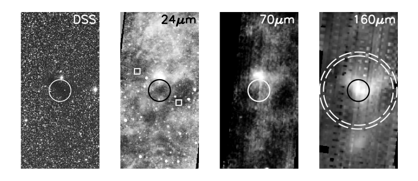
Figure 1.— Gallery of CB$190$ data. The images are centered on the $24\micron$ shadow at RA = $19^{h}20^{m}48^{s}$, Dec = $+23^{o}29\arcmin 45\arcsec$, and are oriented such that north is up and east is to the left. The images have a height of $24\arcmin$ and a width of $12\arcmin$. The corresponding wavelengths are labeled in the top right corners. The optical image is from the red Digital Sky Survey. The original MIPS mosaic pixel scales are $\sim 1\farcs 24$ pix^-1, $9\farcs 8$ pix^-1, and $16\arcsec$ pix^-1, for 24 $\micron$, 70 $\micron$, and 160 $\micron$ respectively. The 24 $\micron$ image displayed here is binned down by a factor of $4$, and the DSS, $70$, and 160 $\micron$ images are re-gridded to the same scale. All four images are marked with a 100$\arcsec$ circle centered on the location of CB$190$. The 24 $\micron$ image is marked with two $\sim 50\arcsec\times 50\arcsec$ boxes indicating the background regions used to estimate the overall uniform background level (see § 3.3 for more details). The 160 $\micron$ image shows the aperture used for the dust mass determination (see § 3.2) indicated a black circle with a radius of $100\arcsec$, and the inner and outer sky annuli radii at $5\farcm 3$ and $6\farcm 4$, both marked as white dashed circles.

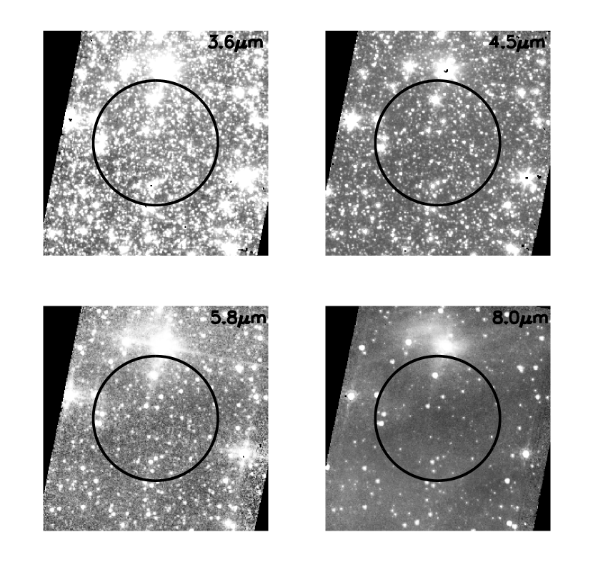
Figure 2.— Gallery of IRAC CB$190$ images centered on the $24\micron$ shadow: RA = $19^{h}20^{m}48^{s}$, Dec = $+23^{o}29\arcmin 45\arcsec$. The images are oriented such that north is up and east is to the left, they are $6\arcmin$ on a side, and the corresponding effective wavelengths of the four IRAC channels are labeled. The original mosaiced IRAC image pixel scale is $0\farcs 6$ pix^-1 and the images displayed here are shown at $1\farcs 2$ pix^-1. The black circles are centered on the 24$\micron$ shadow and have a radius of 100$\arcsec$.

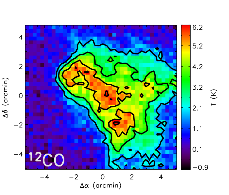
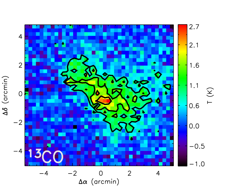
Figure 3.— Maps of the integrated ¹²CO (J = 2-1, $\nu$ = 220.399 GHz) and ¹³CO (J = 2-1, $\nu$ = 230.538 GHz) lines taken with a FWHM telescope resolution of $32\arcsec$ and convolved to a square grid cell spacing of $16\arcsec$. The central coordinates of the images are RA = $19^{h}20^{m}49^{s}$, Dec = $+23^{o}29\arcmin 57\arcsec$. The color-bars indicate the temperature scales in each map. The ¹²CO contour levels are 2, 3.5, 5, and 6 K, and the ¹³CO contour levels are 0.8, 1.4, and 2.0 K.

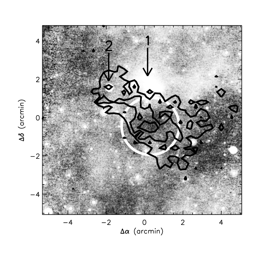
Figure 4.— 24 $\micron$ image with ¹³CO contours overlayed. The image is $\sim\!10\arcmin$ on a side, is centered on the CO map at RA = $19^{h}20^{m}48^{s}$, Dec = $+23^{o}29\arcmin 57\arcsec$, and is displayed at the original mosaic pixel scale of $1\farcs 24$. The ¹³CO contour levels are 0.8, 1.4, and 2.0 K. The white circle is centered on the 24$\micron$ shadow and the peak of the ¹³CO emission. The two arrows indicate two sources that are likely associated with CB$190$; their broad-band SEDs are shown in fig. 8 and discussed in § 3.1.

Figure 5.— High resolution spectra of ¹²CO and ¹³CO J = 2 - 1 lines at the position of the peak CO optical depth, which coincides with the center of the 24 $\mu$m shadow. The spectral resolution of the ¹³CO line is 0.25 MHz or 0.34 km s^-1, and the resolution of the ¹²CO line is 0.05 MHz or 0.061 km s^-1 (R = 5,000,000). The vertical scale of the ¹³CO spectrum is multiplied by 2.5. Total integration time was 15 min on source. RMS noise in the ¹²CO spectrum is 0.12 K (main-beam brightness temperature. The dotted line shows the C¹⁸O J = 2 - 1 spectrum obtained with the Caltech Submillimeter Observatory at a spectral resolution of 0.1 MHz or 0.13 km s^-1 (Michael M. Dunham - private communication, 2006). The vertical scale of the C¹⁸O spectrum is multiplied by 6.

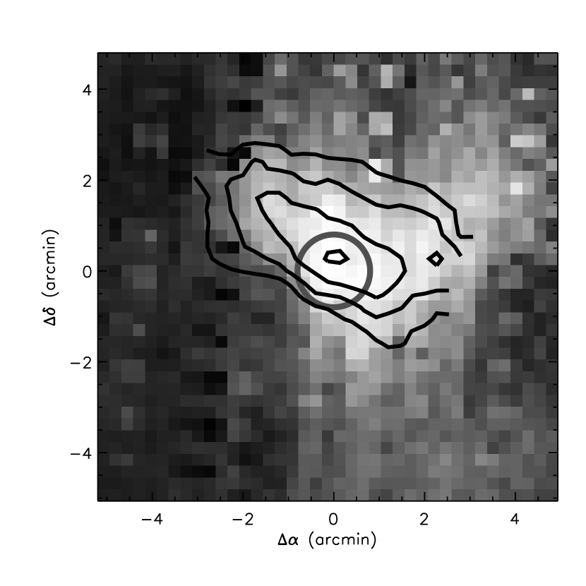
Figure 6.— 160$\micron$ image detail, centered on the 24$\micron$ shadow, with 850$\micron$ contours overlayed in black. The 160$\micron$ image is shown at the original mosaic pixel scale of $16\farcs 0$ pix^-1. The 850$\micron$ contour levels are 0.1, 0.2, 0.3 and 0.4 Jy beam^-1, and the beam is a $32\arcsec$ FWHM Gaussian. The grey circle indicates the location of the 24 $\micron$ shadow and is 48$\arcsec$ in radius.

Figure 7.— 70$\micron$, 160$\micron$, and 850$\micron$ photometry using a 48$\arcsec$ radius aperture centered on the 24$\micron$ shadow coordinates. We show two models for the dust emission with the indicated assumed values of $\beta$ and the corresponding best-fit temperatures.

Figure 8.— F_λ vs. $\lambda$ for three stars: star 1 (HD344204, top), HD1608 (middle), and Vega (bottom). The data extend from 3615Å to 6900Å at 9Å resolution.

Figure 9.— Broad-band SEDs of two sources associated with CB$190$; we show the 2MASS, IRAC and MIPS magnitudes. The $\times$’s show the magnitudes of star 1 (HD344204), at RA = $19^{h}20^{m}47^{s}$, Dec = $23^{o}31\arcmin 40.637\arcsec$. The solid circle indicates the magnitude of star 1 using a large aperture to include the dust emission surrounding the source. The open squares show the magnitudes of star 2, at RA = $19^{h}20m57^{s}$, Dec = $23^{o}31\arcmin 37.6\arcsec$.

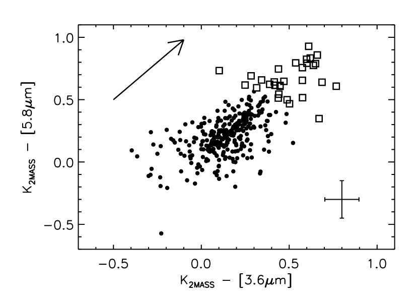
Figure 10.— Color-color plot of stars observed towards CB$190$. We combine 2MASS K-band data with 3.6 $\micron$ and 5.8 $\micron$ IRAC channels. The squares indicate the reddened stars, selected with a 2-$\sigma$ clipping criterion, and the filled circles indicate the unreddened stars. The black arrow shows the best-fit extinction vector slope of 1.2, in good agreement with the Indebetouw et al. (2005) extinction slopes. The median errors for the data are shown in the lower right. The extinction vector derived from the K-[3.6$\micron$] vs. K-[4.5$\micron$] colors also shows good agreement with Indebetouw et al. (2005).

Figure 11.— The radial flux profile for the $24$ $\micron$ shadow. The squares indicate the mean counts per pixel in each $2\farcs 5$ annulus. The chosen truncation radius for the shadow, at $67\farcs 5$ is marked as a solid line; the local background flux level $I_{0}$ is marked with a dashed line.

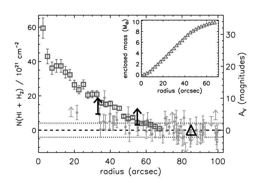
Figure 12.— Comparison of the CB190 column density profiles: the $24$ $\micron$ shadow profile is shown with dark grey squares, and the individual $2$MASS stellar A_V estimates are marked with light grey filled circles. The two dotted lines indicate the 1-$\sigma$ scatter in the 2MASS data just outside the globule, between 70$\arcsec$ and 100$\arcsec$. The black symbols indicate the best-fit Gaussian mean values for the 2MASS data in three radial bins, inside 40$\arcsec$, 40$\arcsec$ to 70$\arcsec$, and 70$\arcsec$ to 100$\arcsec$, and are plotted versus the average radius in each respective bin; the two inner-most points are shown as lower limits (black arrows) because of the inclusion of individual 2MASS lower limits in the best-fit Gaussian calculation. The inset shows the corresponding enclosed mass for the $24$ $\micron$ extinction profile.

Figure 13.— The $24$ $\micron$ column density profile (squares) is shown with the best-fit Bonnor-Ebert model (solid line). The errors in the data are about the size of the squares. The best-fit model parameters are indicated: temperature T $=56.0$ K, $\theta_{max}=69\farcs 0$, and $\xi_{max}=7.2$. The right-hand-side vertical axis indicates the magnitudes of visual extinction, or equivalently, $\tau_{24}$, the optical depth at 24 $\mu$m.

References

- Bacmann et al. (2000) Bacmann, A., André, P., Puget, J.-L., Abergel, A., Bontemps, S., & Ward-Thompson, D. 2000, A&A, 361, 555
- Ballesteros-Paredes et al. (2003) Ballesteros-Paredes, J., Klessen, R. S., & Vázquez-Semadeni, E. 2003, ApJ, 592, 188
- Basu (2004) Basu, S. 2004, in Young Local Universe, Proceedings of XXXIXth Rencontres de Moriond, eds. A. Chalabaev, T. Fukui, T. Montmerle, and J. Tran-Thanh-Van. Paris: Editions Frontieres, ArXiv Astrophysics e-prints, arXiv:astro-ph/0410534
- Bertin & Arnouts (1996) Bertin, E., & Arnouts, S. 1996, A&AS, 117, 393
- Bohlin et al. (1978) Bohlin, R. C., Savage, B. D., & Drake, J. F. 1978, ApJ, 224, 132
- Bonnor (1956) Bonnor, W. B. 1956, MNRAS, 116, 351
- Boss (1997) Boss, A. P. 1997, ApJ, 483, 309
- Chandrasekhar (1939) Chandrasekhar, S. 1939, Chicago, Ill., The University of Chicago press [1939],
- Clemens & Barvainis (1988) Clemens, D. P., & Barvainis, R. 1988, ApJS, 68, 257
- Crutcher et al. (1994) Crutcher, R. M., Mouschovias, T. C., Troland, T. H., & Ciolek, G. E. 1994, ApJ, 427, 839
- Dame & Thaddeus (1985) Dame, T. M., & Thaddeus, P. 1985, ApJ, 297, 751
- Draine (2003a) Draine, B. T. 2003a, ARA&A, 41, 241
- Draine (2003b) Draine, B. T. 2003b, ApJ, 598, 1017
- Ebert (1955) Ebert, R. 1955, Zeitschrift fur Astrophysik, 36, 222
- Evans et al. (2001) Evans, N. J., Rawlings, J. M. C., Shirley, Y. L., & Mundy, L. G. 2001, ApJ, 557, 193
- Fazio et al. (2004) Fazio, G. G., et al. 2004, ApJS, 154, 10
- Gordon et al. (2005) Gordon, K. D., et al. 2005, PASP, 117, 503
- Gordon et al. (2006) Gordon, K. D., et al. 2006, ApJ, 638, L87
- Gutermuth et al. (2004) Gutermuth, R. A., Megeath, S. T., Muzerolle, J., Allen, L. E., Pipher, J. L., Myers, P. C., & Fazio, G. G. 2004, ApJS, 154, 374
- Harris et al. (1978) Harris, D. H., Woolf, N. J., & Rieke, G. H. 1978, ApJ, 226, 829
- Harvey et al. (2003) Harvey, D. W. A., Wilner, D. J., Lada, C. J., Myers, P. C., & Alves, J. F. 2003, ApJ, 598, 1112
- Henry et al. (2003) Henry, T. J., Backman, D. E., Blackwell, J., Okimura, T., & Jue, S. 2003, The Future of Small Telescopes In The New Millennium. Volume III - Science in the Shadow of Giants, 111
- Hotzel et al. (2002) Hotzel, S., Harju, J., & Juvela, M. 2002, A&A, 395, L5
- Indebetouw & Zweibel (2000) Indebetouw, R., & Zweibel, E. G. 2000, ApJ, 532, 361
- Indebetouw et al. (2005) Indebetouw, R., et al. 2005, ApJ, 619, 931
- Jijina et al. (1999) Jijina, J., Myers, P. C., & Adams, F. C. 1999, ApJS, 125, 161
- Kandori et al. (2005) Kandori, R., et al. 2005, AJ, 130, 2166
- Kirk et al. (2007) Kirk, J. M., Ward-Thompson, D., & André, P. 2007, MNRAS, 375, 843
- Kulesa et al. (2005) Kulesa, C. A., Hungerford, A. L., Walker, C. K., Zhang, X., & Lane, A. P. 2005, ApJ, 625, 194
- Kutner & Ulich (1981) Kutner, M. L., & Ulich, B. L. 1981, ApJ, 250, 341
- Lada et al. (2004) Lada, C. J., Huard, T. L., Crews, L. J., & Alves, J. F. 2004, ApJ, 610, 3
- Lee et al. (2003) Lee, J.-E., Evans, N. J., II, Shirley, Y. L., & Tatematsu, K. 2003, ApJ, 583, 789
- Lemme et al. (1996) Lemme, C., Wilson, T. L., Tieftrunk, A. R., & Henkel, C. 1996, A&A, 312, 585
- Lynds (1962) Lynds, B. T. 1962, ApJS, 7, 1
- Milam et al. (2005) Milam, S. N., Savage, C., Brewster, M. A., Ziurys, L. M., & Wyckoff, S. 2005, ApJ, 634, 1126
- Neckel et al. (1980) Neckel, T., Klare, G., & Sarcander, M. 1980, A&AS, 42, 251
- Ossenkopf & Henning (1994) Ossenkopf, V., & Henning, T. 1994, A&A, 291, 943
- Press et al. (1992) Press, W. H., Teukolsky, S. A., Vetterling, W. T., & Flannery, B. P. 1992, Cambridge: University Press, —c1992, 2nd ed
- Rieke & Lebofsky (1985) Rieke, G. H., & Lebofsky, M. J. 1985, ApJ, 288, 618
- Rieke et al. (2004) Rieke, G. H., et al. 2004, ApJS, 154, 25
- Rodríguez et al. (2007) Rodríguez, L. F., Zapata, L. A., & Ho, P. T. P. 2007, ApJ, 654, L143
- Rohlfs & Wilson (2004) Rohlfs, K., & Wilson, T. L. 2004, Tools of radio astronomy, 4th rev. and enl. ed., by K. Rohlfs and T.L. Wilson. Berlin: Springer, 2004
- Sault et al. (1995) Sault R.J., Teuben P.J., Wright M.C.H., 1995, in Astronomical Data Analysis Software and Systems IV, ed. R. Shaw, H.E. Payne, J.J.E. Hayes, ASP Conf. Ser., 77, 433-436
- Shirley et al. (2005) Shirley, Y. L., Nordhaus, M. K., Grcevich, J. M., Evans, N. J., Rawlings, J. M. C., & Tatematsu, K. 2005, ApJ, 632
- Sigalotti & Klapp (2000) Sigalotti, L. D. G., & Klapp, J. 2000, ApJ, 531, 1037
- Skrutskie et al. (2006) Skrutskie, M. F., et al. 2006, AJ, 131, 1163
- Stahler & Palla (2005) Stahler, S. W., & Palla, F. 2005, The Formation of Stars, by Steven W. Stahler, Francesco Palla, pp. 865. ISBN 3-527-40559-3. Wiley-VCH , January 2005
- Tafalla et al. (2002) Tafalla, M., Myers, P. C., Caselli, P., Walmsley, C. M., & Comito, C. 2002, ApJ, 569, 815
- Tassis & Mouschovias (2004) Tassis, K., & Mouschovias, T. C. 2004, ApJ, 616, 283
- Teixeira et al. (2005) Teixeira, P. S., Lada, C. J., & Alves, J. F. 2005, ApJ, 629, 276
- Visser et al. (2002) Visser, A. E., Richer, J. S., & Chandler, C. J. 2002, AJ, 124, 2756
- Weingartner & Draine (2001) Weingartner, J. C., & Draine, B. T. 2001, ApJ, 548, 296
- Witt et al. (1990) Witt, A. N., Oliveri, M. V., & Schild, R. E. 1990, AJ, 99, 888
- Whitney et al. (2003) Whitney, B. A., Wood, K., Bjorkman, J. E., & Cohen, M. 2003, ApJ, 598, 1079
- Whittet (2003) Whittet, D. C. B. 2003, Dust in the galactic environment, 2nd ed. by D.C.B. Whittet. Bristol: Institute of Physics (IOP) Publishing, 2003 Series in Astronomy and Astrophysics, ISBN 0750306246