Electrodynamics of the Josephson vortex lattice in high-temperature superconductors

Abstract

We studied the response of the Josephson vortex lattice in layered superconductors to the high-frequency c-axis electric field. We found a simple relation connecting the dynamic dielectric constant with the perturbation of the superconducting phase, induced by oscillating electric field. Numerically solving equations for the oscillating phases, we computed the frequency dependences of the loss function at different magnetic fields, including regions of both dilute and dense Josephson vortex lattices. The overall behavior is mainly determined by the c-axis and in-plane dissipation parameters, which are inversely proportional to the anisotropy. The cases of weak and strong dissipations are realized in $\mathrm{Bi_{2}Sr_{2}CaCu_{2}O_{x}}$ and underdoped $\mathrm{YBa_{2}Cu_{3}O_{x}}$, respectively. The main feature of the response is the Josephson-plasma-resonance peak. In the weak-dissipation case additional satellites appear in the dilute regime in the higher-frequency region due to the excitation of the plasma modes with the wave vectors set by the lattice structure. In the dense-lattice limit the plasma peak moves to a higher frequency and its intensity rapidly decreases, in agreement with experiment and analytical theory. The behavior of the loss function at low frequencies is well described by the phenomenological theory of vortex oscillations. In the case of very strong in-plane dissipation an additional peak in the loss function appears below the plasma frequency. Such peak has been observed experimentally in underdoped $\mathrm{YBa_{2}Cu_{3}O_{x}}$. It is caused by the frequency dependence of the in-plane contribution to losses rather than a definite mode of phase oscillations.

I Introduction

The Josephson plasma resonance (JPR)art93 ; TKTPRB94 ; bmtPRL95 is one of the most prominent manifestations of the intrinsic Josephson effect in layered superconductors.IJJReviews ; YurgensReview It has been established as a valuable tool to study the intrinsic properties of superconductorsGaifullinPRL99 ; DordevicPRB05 and it was extensively used to probe different states of vortex matter.OngJPR ; MatsudaJPR ; KadowJPR ; ShibauchiPRL99 ; vdBeek ; DulicPRL01 ; Thorsmolle The value of the JPR frequency depends on the anisotropy factor and it ranges widely for different compounds, from several hundred gigahertz in $\mathrm{Bi_{2}Sr_{2}CaCu_{2}O_{x}}$ (BSCCO) to several terahertz in underdoped $\mathrm{YBa_{2}Cu_{3}O_{x}}$ (YBCO).

An interesting issue is the influence of the magnetic field applied along the layer direction on the high-frequency response and, in particular, on the JPR. Such field forms the lattice of Josephson vortices (JVL). The anisotropy factor, $\gamma$, and the interlayer periodicity, $s$, set the important field scale, $B_{\mathrm{cr}}=\Phi_{0}/(2\pi\gamma s^{2})$. At $B<B_{\mathrm{cr}}$ the Josephson vortices are well separated and form a dilute lattice. When the magnetic field exceeds $B_{\mathrm{cr}}$ the Josephson vortices homogeneously fill all layers (dense-lattice regime).BulClemPRB91 ; KoshGrState ; NonomHuPRB06 The crossover field ranges from $\sim$0.5 tesla for BSCCO to $\sim$10 tesla for underdoped YBCO. The JVL state is characterized by a very rich spectrum of dynamic properties. In particular, the transport properties of the JVL in BSCCO have been extensively studied by several experimental groups.Lee ; Hechtfischer ; Latyshev

The high-frequency response in the magnetic fields along the layers has been studied experimentally in BSCCO using the microwave absorption in cavity resonators KakeyaPRB05 , in $\mathrm{La_{2-x}Sr_{x}CuO_{4}}$ DordevicPRB05 , and in underdoped YBCO KojimaJLTP03 ; LaForge by the infrared reflection spectroscopy. A detailed comparison between the behaviors of the high-frequency response in the in-plane magnetic field for these compounds has been made recently by LaForge et al.LaForge In BSCCO, two resonance absorption peaks have been observed.KakeyaPRB05 The upper-resonance frequency increases with the field and approaches the JPR frequency at small fields, while the lower-resonance frequency decreases with the field and approaches approximately half of the JPR frequency at small fields. In the underdoped YBCOKojimaJLTP03 ; LaForge , the JPR peak in the loss function rapidly loses its intensity with increasing the field, while the resonance frequency either does not move or slowly increases with the field. In addition, another wide peak emerges at a smaller frequency and its intensity increases with increasing field.

Several theoretical approaches have been used to describe the response of the JVL state to the oscillating electric field. A phenomenological vortex-oscillation theory has been proposed by Tachiki et al. TKTPRB94 . This theory describes the response of the JVL at small frequencies and fields, in terms of phenomenological vortex parameters, mass, viscosity coefficient, and pinning spring constant. This approach is expected to work at frequencies much smaller then the JPR frequency, i.e., it can not be used to describe the JPR peak itself.

On the other hand, the plasmon spectrum at high magnetic fields, in the dense-lattice limit, has been calculated by Bulaevskii et al. BulPRB97 It was found that the plasma mode at zero wave vector increases proportionally to the magnetic field, $\omega_{p}(B)=\omega_{p}(0)B/(2B_{\mathrm{cr}})$. This prediction describes very well the behavior of the high-frequency mode in BSCCO.KakeyaPRB05 A more quantitative numerical study of the JVL plasma modes in the dense-lattice regime has been done by Koyama.KoyamaPRB03 He reproduced the mode, linearly growing with field, and also found additional modes at smaller frequencies.

In this paper we develop a quantitative description of the high-frequency response for a homogenous layered superconductor valid for whole range of frequencies and fields. We relate the dynamic dielectric constant via simple averages of the oscillating phases. The high-frequency response is mainly determined by the c-axis and in-plane dissipation parameters, which are inversely proportional to the anisotropy. Analytical results for the dynamic dielectric constant and loss function can be derived in limiting cases, at small fields and frequencies (vortex-oscillation regime) and at high fields, in the dense-lattice regime. Numerically solving dynamic equations for the oscillating phases, we studied applicability limits of the approximate analytical results and investigated the influence of the dissipation parameters on the shape of the loss function. Computing the oscillating phases for different vortex lattices, we traced the field evolution of the loss function with increasing magnetic field for the cases of weak and strong dissipations, typical for BSCCO and underdoped YBCO, respectively.

II Dynamic phase equations, dielectric constant, and loss function

The equations describing phase dynamics in layered superconductors can be derived from Maxwell’s equations expressing fields and currents in terms of the gauge invariant phase difference between the layers $\theta_{n}=\phi_{n+1}-\phi_{n}-\left(2\pi s/\Phi_{0}\right)A_{z}$. These equations have been presented in several different forms.Inductive We will use them in the form of coupled equations for the phase differences and magnetic field when charging effects can be neglected, see, e.g., Refs. ArtJETPL97, ; KoshAranPRB01, ,

$$\frac{\sigma_{c}\Phi_{0}}{2\pi csj_{J}}\frac{\partial\theta_{n}}{\partial t}\!+\!\sin\theta_{n}\!+\!\frac{1}{\omega_{p}^{2}}\frac{\partial^{2}\theta_{n}}{\partial t^{2}}\!-\!\frac{c}{4\pi j_{J}}\frac{\partial B_{n}}{\partial x}\!=\!\frac{1}{4\pi j_{J}}\frac{\partial\mathcal{D}_{z}}{\partial t},$$ (1a)

$$\left(\frac{4\pi\sigma_{ab}}{c^{2}}\frac{\partial}{\partial t}+\frac{1}{\lambda_{ab}^{2}}\right)\left(\frac{\Phi_{0}}{2\pi s}\frac{\partial\theta_{n}}{\partial x}-B_{n}\right)=-\frac{\nabla_{n}^{2}B_{n}}{s^{2}},$$ (1b)

where the magnetic field is along the $$y \sigma_{ab} \sigma_{c} \lambda_{ab} \lambda_{c} j_{J}=c\Phi_{0}/(8\pi^{2}s\lambda_{c}^{2}) \omega_{p}=c/\sqrt{\varepsilon_{c}}\lambda_{c} \mathcal{D}_{z} \nabla_{n}^{2}B_{n}\equiv B_{n+1}+B_{n-1}-2B_{n}$$ axis, and are the components of the quasiparticle conductivity, and are the components of the London penetration depth, is the Josephson current density, is the plasma frequency, is the external electric field, and . Neglecting charging effects charging , the local electric field is connected with the phase difference by the Josephson relation,

$$E_{z}\approx\frac{\Phi_{0}}{2\pi cs}\frac{\partial\theta_{n}}{\partial t}.$$ (2)

The average magnetic induction inside the superconductor, $B_{y}$, fixes the average phase gradient, $\left\langle\partial\theta_{n}^{(0)}/\partial x\right\rangle=2\pi sB_{y}/\Phi_{0}$.

To facilitate analysis, we use a standard transformation to the reduced variables,

$$x/\lambda_{J}\rightarrow x,\ \ t\omega_{p}\rightarrow t,\ \ h_{n}=2\pi\gamma s^{2}B_{n}/\Phi_{0},$$

with $\lambda_{J}=\gamma s$, and introduce the dimensionless parameters

$$l=\frac{\lambda_{ab}}{s},\ \nu_{c}=\frac{4\pi\sigma_{c}}{\varepsilon_{c}\omega_{p}},\ \nu_{ab}=\frac{4\pi\sigma_{ab}\lambda_{ab}^{2}\omega_{p}}{c^{2}}.$$

It is important to note that both damping parameters, $\nu_{c}$ and $\nu_{ab}$, roughly scale inversely proportional to the anisotropy factor $\gamma$, meaning that the effective damping is stronger in less anisotropic materials. In particular, the cases of weak and strong dissipation are realized in BSCCO and underdoped YBCO, respectively. Due to the d-wave pairing in the high-temperature superconductors, both dissipation parameters do not vanish at $T\rightarrow 0$. Another important feature of the high-temperature superconductors is that the in-plane dissipation is typically much stronger than the c-axis dissipation, $\nu_{ab}\gg\nu_{c}$.LatyshevKBPRB03 This is a consequence of a rapid decrease of the in-plane scattering rate with decreasing temperature, which manifests itself as a large peak in the temperature dependence of the in-plane quasiparticle conductivity.quasiYBCO ; quasiBSCCO

Assuming an oscillating external field and using a complex presentation, $\mathcal{D}_{z}(t)=\mathcal{D}_{z}\exp(-i\omega t)$, we obtain for small oscillations

$$\left(-i\nu_{c}\tilde{\omega}+C_{n}(x)-\tilde{\omega}^{2}\right)\theta_{n}-l^{2}\frac{\partial h_{n}}{\partial x} =\frac{i\omega}{4\pi j_{J}}\mathcal{D}_{z}$$ (3a)

$$\frac{\partial\theta_{n}}{\partial x}-h_{n}+\frac{l^{2}}{1-i\nu_{ab}\tilde{\omega}}\nabla_{n}^{2}h_{n} =0$$ (3b)

where $$\tilde{\omega}=\omega/\omega_{p} C_{n}(x)\equiv\cos[\theta_{n}^{(0)}(x)] \theta_{n}^{(0)}(x)$$, , and the static phases, , are determined by the following reduced equations

$$\frac{\partial^{2}\theta_{n}^{(0)}}{\partial x^{2}}+\left(-\frac{1}{l^{2}}+\Delta_{n}\right)\sin\theta_{n}^{(0)}=0$$ (4)

with the addition condition $\left\langle\partial\theta_{n}^{(0)}/\partial x\right\rangle=h=2\pi\gamma s^{2}B_{y}/\Phi_{0}$. We introduce the reduced oscillating phase $\vartheta_{n}$,

$$\theta_{n}=\vartheta_{n}\frac{\omega_{p}\mathcal{D}_{z}}{4\pi j_{J}},$$

for which we can derive from Eqs. (3a) and (3b) the following reduced equation

$$- \frac{\partial^{2}\vartheta_{n}}{\partial x^{2}}+\left(\frac{1}{l^{2}}-\frac{1}{1-i\nu_{ab}\tilde{\omega}}\nabla_{n}^{2}\right)$$

$$\times\left[C_{n}(x)-\tilde{\omega}^{2}-i\nu_{c}\tilde{\omega}\right]\vartheta_{n}=-\frac{i\tilde{\omega}}{l^{2}}.$$ (5)

From the Josephson relation (2) we find $E_{z}=\left(-i\tilde{\omega}/\varepsilon_{c}\right)\overline{\vartheta}\mathcal{D}_{z}$, meaning that the dynamic dielectric constant is connected with the average reduced oscillating phase, $\overline{\vartheta}$, by a simple relation

$$\varepsilon_{c}(\tilde{\omega})=-\varepsilon_{c}/(i\tilde{\omega}\overline{\vartheta}).$$ (6)

Consider the case of a zero magnetic field first. In this case $\theta_{n}^{(0)}(x)=0$ and the oscillating phase is given by

$$\vartheta_{n}=\overline{\vartheta}=\frac{-i\tilde{\omega}}{1-\tilde{\omega}^{2}-i\nu_{c}\tilde{\omega}}.$$ (7)

In this case Eq. (6) gives well-known results for the dynamic dielectric constant, $\varepsilon_{c0}(\omega)\equiv\mathcal{D}_{z}/E_{z}$, and the loss function, $L_{0}(\omega)=\operatorname{Im}[-1/\varepsilon_{c0}(\omega)]$ at the zero magnetic field, which we present in real units,

$$\varepsilon_{c0}(\omega) =\varepsilon_{c}-\frac{\varepsilon_{c}\omega_{p}^{2}}{\omega^{2}}+\frac{4\pi i\sigma_{c}}{\omega},$$ (8)

$$L_{0}(\omega) =\frac{4\pi\omega^{3}\sigma_{c}/\varepsilon_{c}^{2}}{\left(\omega^{2}-\omega_{p}^{2}\right)^{2}+\left(4\pi\omega\sigma_{c}/\varepsilon_{c}\right)^{2}}.$$ (9)

The zero-field loss function has a peak at the Josephson plasma frequency with width determined only by the c-axis quasiparticle conductivity.

Consider now the case of a finite magnetic field applied in the layer direction. Such magnetic field generates the lattice of the Josephson vortices, which is described by the static phase distribution, $\theta_{n}^{(0)}(x)$, obeying Eq. (4). The oscillating phase, in turn, is fully determined by this phase via the spatial distribution of the average cosine, $C_{n}(x)$. Averaging Eq. (4), we obtain an obvious identity $\langle\sin\theta_{n}^{(0)}\rangle=0$, indicating that there is no average current in the ground state. In the field range $B_{y}\gg\Phi_{0}/2\pi\lambda_{ab}\lambda_{c}$ the term $1/l^{2}$ can be neglected. In this limit it is more convenient to operate with the in-plane phases $\phi_{n}^{(0)}(x)$, defined by the relation $\theta_{n}^{(0)}=\phi_{n+1}^{(0)}-\phi_{n}^{(0)}+hx$, which obey the following equation

$$\frac{\partial^{2}\phi_{n}^{(0)}}{\partial x^{2}} +\sin\left(\phi_{n+1}^{(0)}-\phi_{n}^{(0)}+hx\right)$$

$$-\sin\left(\phi_{n}^{(0)}-\phi_{n-1}^{(0)}+hx\right)=0.$$ (10)

Due to the translational invariance, every solution $\phi_{n}^{(0)}(x)$ generates a continuous family of solutions $\phi_{n}^{(0)}(x-u)$ corresponding to the lattice shifts $u$. In particular, the phase change for a small displacement is given by $\delta\phi_{n}\!=\!-u\partial\phi_{n}^{(0)}/\partial x$. Taking the $x$-derivative of Eq. (10), we find that $\partial\phi_{n}^{(0)}/\partial x$ obeys the following equation

$$\frac{\partial^{3}\phi_{n}^{(0)}}{\partial x^{3}}+C_{n}\frac{\partial\phi_{n+1}^{(0)}}{\partial x}+C_{n-1}\frac{\partial\phi_{n-1}^{(0)}}{\partial x}$$

$$-\left(C_{n}+C_{n-1}\right)\frac{\partial\phi_{n}^{(0)}}{\partial x}=-\nabla_{n}C_{n}h$$ (11)

with $C_{n}=\cos\left(\phi_{n+1}^{(0)}-\phi_{n}^{(0)}+hx\right)$ and $\nabla_{n}C_{n}=C_{n}-C_{n-1}$. The condition $\left\langle\partial\sin\theta_{n}^{(0)}/\partial x\right\rangle=0$ gives another useful identity for $\partial\phi_{n}^{(0)}/\partial x$

$$\overline{C_{n}\left(\frac{\partial\phi_{n+1}^{(0)}}{\partial x}-\frac{\partial\phi_{n}^{(0)}}{\partial x}\right)}=-Ch.$$ (12)

We now proceed with the analysis of the dynamic phase equation (5). Averaging this equation, we obtain the following relation

$$\left(i\nu_{c}\omega+\omega^{2}\right)\overline{\vartheta}-\overline{C_{n}(x)\vartheta_{n}}=i\omega.$$

Splitting $\vartheta_{n}(x)$ into the average and oscillating-in-space parts, $\vartheta_{n}(x)=\overline{\vartheta}\left(1+w_{n}(x)\right)$, with $\overline{w_{n}(x)}=0$, we obtain

$$\overline{\vartheta}=\frac{i\tilde{\omega}}{\omega^{2}-C-\overline{C_{n}(x)w_{n}}+i\nu_{c}\tilde{\omega}}.$$

Using relation (6), we obtain the following result for the dielectric constant

$$\frac{\varepsilon_{c}}{\varepsilon_{c}(\tilde{\omega})}=\frac{\tilde{\omega}^{2}}{\tilde{\omega}^{2}-C-\overline{C_{n}(x)w_{n}}+i\nu_{c}\tilde{\omega}}.$$ (13)

Therefore, the dynamic dielectric constant is fully determined by the two simple averaged quantities, the static average cosine, $C$, and the average including the spatial distribution of the oscillating phase, $\overline{C_{n}(x)w_{n}}$.

Introducing again the in-plane oscillating phases, $w_{n}=\phi_{n+1}-\phi_{n}$, and neglecting terms of the order of $1/l^{2}$, we derive the following equation

$$\frac{\partial^{2}\phi_{n}}{\partial x^{2}} +\frac{1}{1-i\nu_{ab}\tilde{\omega}}\nabla_{n}\left[C_{n}(x)-\tilde{\omega}^{2}-i\nu_{c}\tilde{\omega}\right]\nabla_{n}\phi_{n}$$

$$=-\frac{\nabla_{n}C_{n}(x)}{1-i\nu_{ab}\tilde{\omega}}.$$ (14)

The oscillating phase has the same symmetry properties as the vortex lattice. Comparing this equation with Eq. (11), we see that in the limit $\omega\rightarrow 0$ the solution is given by

$$\phi_{n}\rightarrow\frac{1}{h}\frac{\partial\phi_{n}^{(0)}}{\partial x}.$$ (15)

This solution corresponds to the homogeneous lattice shift. As follows from Eq. (12), the combination $C+\overline{C_{n}(x)w_{n}}=C+\overline{C_{n}(x)\left(\phi_{n+1}-\phi_{n}\right)}$, which determines the dielectric constant (13), vanishes in this limit. This property is a consequence of the translational invariance and it is only true in the absence of pinning of the vortex lattice.

In summary, to find the dynamic dielectric constant at a given field, one has to find first the static phase from Eq. (10) assuming a definite vortex-lattice structure and compute the average cosine, $C=\left\langle\cos\left(\phi_{n+1}^{(0)}-\phi_{n}^{(0)}+hx\right)\right\rangle$. After that, one has to solve the dynamic equation (14) and compute the average $\overline{C_{n}(x)w_{n}}\!=\!\overline{C_{n}(x)\left(\phi_{n+1}\!-\!\phi_{n}\right)}$. These two averages completely determine $\varepsilon_{c}(\omega)$ via Eq. (13). In the following sections, we will consider regimes in which analytical solutions are possible, the high-field limit and the vortex-oscillation regime at small frequencies. Then, we will present the results of the numerical analysis in the full field and frequency range in the cases of weak dissipation (BSCCO) and large dissipation (underdoped YBCO).

III High-field regime

In this section we consider the high-field regime, $h\gg 1$, corresponding to the dense-lattice limit in which all interlayer junctions are homogeneously filled with vortices. This regime allows for the full analytical description using an expansion with respect to the Josephson currents. In particular, the spectrum of the plasma modes and their damping in this limit have been found by Bulaevskii et al.BulPRB97 We use the same approach to derive the dynamic dielectric constant.

The static phase solution at high fields, describing the triangular lattice, is given by

$$\phi_{n}^{(0)}\approx\frac{\pi n(n-1)}{2}+\frac{2}{h^{2}}\sin\left(hu+\pi n\right).$$ (16)

Using this distribution, we compute the average cosine

$$C\approx\overline{\cos\left[hu+\pi n-\frac{4}{h^{2}}\sin\left(hu+\pi n\right)\right]}\approx\frac{2}{h^{2}}.$$ (17)

At high fields we can neglect rapidly oscillating $C_{n}(x)$ in the right hand side of Eq. (14). This allows us to obtain the solution

$$\phi_{n}=-\frac{C_{n}(x)/2}{\tilde{\omega}^{2}-\left(1-i\nu_{ab}\tilde{\omega}\right)h^{2}/4+i\nu_{c}\tilde{\omega}},$$ (18)

compute the average

$$\overline{C_{n}(x)\left(\phi_{n+1}-\phi_{n}\right)}=\frac{1/2}{\tilde{\omega}^{2}-\left(1-i\nu_{ab}\tilde{\omega}\right)h^{2}/4+i\nu_{c}\tilde{\omega}},$$

and, finally, obtain the high-field limit of $\varepsilon_{c}(\omega)$ from Eq. (13),

$$\frac{\varepsilon_{c}(\tilde{\omega})}{\varepsilon_{c}}\!\approx\!1\!+\!\frac{i\nu_{c}}{\tilde{\omega}}\!-\!\frac{2}{h^{2}\tilde{\omega}^{2}}\!-\!\frac{1/(2\tilde{\omega}^{2})}{\tilde{\omega}^{2}\!+\!i\nu_{c}\tilde{\omega}\!-\!\left(1\!-\!i\nu_{ab}\tilde{\omega}\right)h^{2}\!/4}.$$ (19)

In the low-damping regime $\nu_{c},\nu_{ab}\ll 1$ the loss function has a peak at $\tilde{\omega}=h/2$ (in real units $\omega=\omega_{p}\pi\gamma s^{2}B_{y}/\Phi_{0}$) corresponding to the homogeneous plasma mode.BulPRB97 Such linear growth of the plasma frequency with field has been indeed observed experimentally in underdoped BSCCO by Kakeya et al. KakeyaPRB05

To verify the accuracy of the high-field approximation (19), we compare in Fig. 1 the loss function obtained from this formula with an accurate numerical solution for two field values, $h=2$ and $4$ in the case of weak dissipation, $\nu_{c}=0.01$ and $\nu_{ab}=0.1$. One can see that the high-field formula accurately describes the low-frequency region already at $h=2$, but it overestimates the peak frequency. At $h=4$ the high-frequency approximation is already undistinguishable from the exact result.

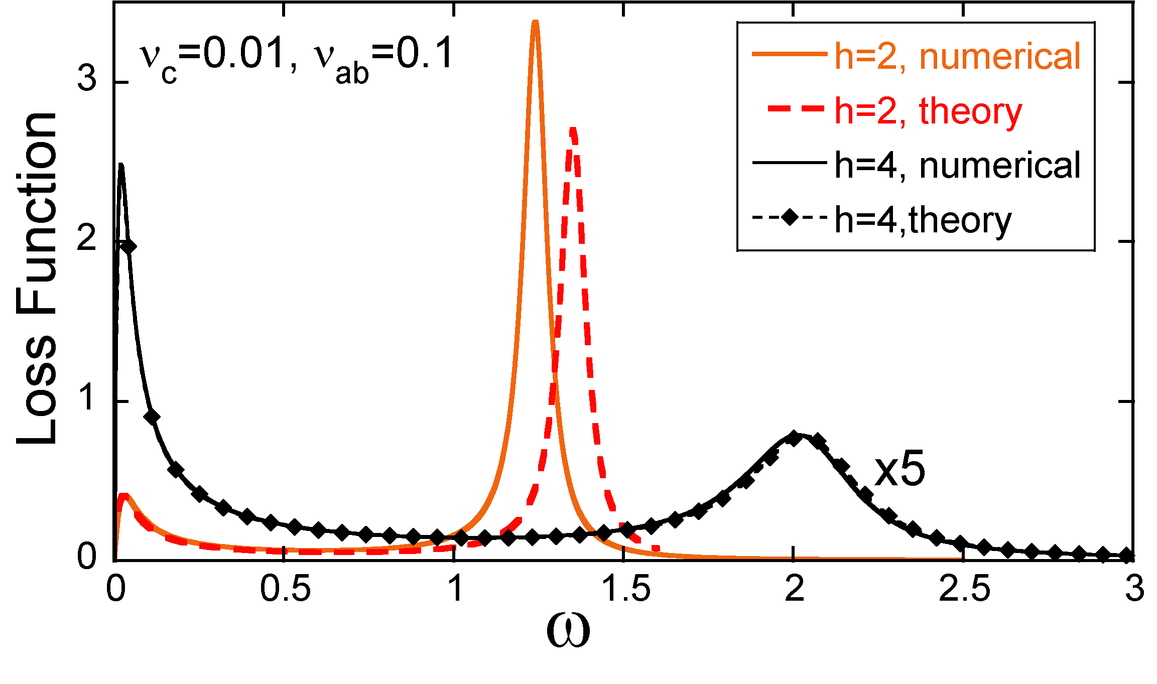
Figure 1: (Color online) Comparison between the approximate high-field limit of the loss function based on Eq. (19) and exact numerical solution for two field values, $h=2$ and $4$ in the case of weak dissipation, $\nu_{c}=0.01$ and $\nu_{ab}=0.1$. For clarity, the vertical scale for the $h=4$ plots is magnified 5 times.

IV Vortex-oscillations regime at small fields and frequencies

In this section we consider the phenomenological theory of vortex oscillations which describes the response of the vortex lattice at small frequencies, $\omega\ll\omega_{p}$. For the Abrikosov vortex lattice such a theory was developed by Coffey and Clem.CoffeyClemPRB92 The dynamic dielectric constant for the Josephson vortex lattice has been derived using a similar approach by Tachiki, Koyama, and Takahashi.TKTPRB94

Consider a superconductor in the vortex state carrying ac supercurrent $j_{s}\propto\exp(-i\omega t)$ along the $c$ axis. The ac electric field consists of the London term and the contribution from the vortex oscillations,

$$E_{z}=-\frac{4\pi\lambda_{c}^{2}}{c^{2}}i\omega j_{s}-\frac{B_{y}}{c}i\omega u.$$ (20)

The vortex oscillation amplitude, $u$, can be found from the equation

$$\left(-\rho_{J}\omega^{2}-i\eta_{J}\omega+K\right)u=\frac{\Phi_{0}}{c}j_{s},$$ (21)

where $\rho_{J}$ is the linear mass of the Josephson vortex CoffeyClemVMassPRB92 , $\eta_{J}$  is its viscosity coefficient CoffeyClemJViscPRB90 ; JVflux-flow , and $K$ is the spring constant due to pinning (it is neglected in the rest of the paper). In Appendix A we present formulas for $\rho_{J}$ and $\eta_{J}$ in terms of superconductor parameters. Finding the oscillating amplitude, we obtain

$$E_{z}=-\left(4\pi\lambda_{c}^{2}+\frac{B_{y}\Phi_{0}}{-\rho_{J}\omega^{2}-i\eta_{J}\omega+K}\right)\frac{i\omega j_{s}}{c^{2}}.$$ (22)

A finite electric field also generates the quasiparticle current $j_{n}=\sigma_{c,n}(\omega)E_{z}$. Therefore, the total conductivity $\sigma_{c}(B_{y},\omega)=(j_{s}+j_{n})/E_{z}$ is given by

$$\sigma_{c}(B_{y},\omega)= \sigma_{c,n}(\omega)$$

$$- \frac{\varepsilon_{c}\omega_{p}^{2}}{4\pi i\omega}\left(1\!+\!\frac{1}{-\!\rho_{J}\omega^{2}\!-\!i\eta_{J}\omega\!+\!K}\frac{B_{y}\Phi_{0}}{4\pi\lambda_{c}^{2}}\right)^{-1}.$$ (23)

The interesting feature of the real part of conductivity,

$$\sigma_{c,1}(B_{y},\omega) =\operatorname{Re}[\sigma_{c,n}(\omega)]$$

$$+\frac{\eta_{J}\varepsilon_{c}\omega_{p}^{2}B_{y}\Phi_{0}/\left(4\pi\lambda_{c}\right)^{2}}{\left(K\!+\!B_{y}\Phi_{0}/(4\pi\lambda_{c}^{2})-\!\rho_{J}\omega^{2}\right)^{2}\!+\!\left(\eta_{J}\omega\right)^{2}},$$ (24)

is a resonance peak at the frequency $\omega_{r}=\sqrt{\left[K\!+\!B_{y}\Phi_{0}/(4\pi\lambda_{c}^{2})\right]/\rho_{J}}$. As one can see from Eq. (22), this resonance is a result of compensation of the London and vortex contributions to the oscillating electric field at $\omega\sim\omega_{r}$. Using the result for the vortex linear mass $\rho_{J}$ from Appendix A and neglecting pinning, the formula for $\omega_{r}$ can be rewritten more transparently as $\omega_{r}\approx 0.84\omega_{p}\sqrt{2\pi\gamma s^{2}B_{y}/\Phi_{0}}$. At $\omega\rightarrow 0$, Eq. (24) gives a known result for the dc flux-flow conductivity.JVflux-flow

Using the well-known relation between the dynamic dielectric constant and conductivity, $\varepsilon_{c}(\omega)=\varepsilon_{c}-4\pi\sigma_{c}(\omega)/i\omega$, we obtain TKTPRB94

$$\varepsilon_{c}(B_{y},\omega)= \varepsilon_{c}\!-\!\frac{4\pi\sigma_{c,n}(\omega)}{i\omega}$$

$$-\frac{\varepsilon_{c}\omega_{p}^{2}}{\omega^{2}}\left(1\!+\!\frac{1}{-\rho_{J}\omega^{2}\!-\!i\eta_{J}\omega\!+\!K}\frac{B_{y}\Phi_{0}}{4\pi\lambda_{c}^{2}}\right)^{-1}.$$ (25)

Using again formulas for $\rho_{J}$ and $\eta_{J}$ from Appendix A and neglecting pinning, we rewrite this result in reduced variables in the form, convenient for comparison with numerical calculations,

$$\frac{\varepsilon_{c}(h,\tilde{\omega})}{\varepsilon_{c}}=1\!+\!\frac{i\nu_{c}}{\tilde{\omega}}\!-\!\frac{1/\tilde{\omega}^{2}}{1\!-\!2\pi h/[C_{c}(\tilde{\omega}^{2}\!+\!i\nu_{c}\tilde{\omega})\!+\!C_{ab}i\nu_{ab}\tilde{\omega}]}$$ (26)

with $C_{c}\approx 9.0$ and $C_{ab}\approx 2.4$. We remind that this formula is valid only at small fields, $h\ll 1$, and frequencies, $\tilde{\omega}\ll 1$.

V Field evolution of the Loss Function

In the full range of frequencies and fields, the dynamic dielectric function can only be computed numerically. At the first step, one has to find the static phase distribution from Eq. (10) assuming a definite vortex lattice structure. To probe general trends, we limit ourselves here only by simple aligned lattices. At a fixed magnetic field, such a lattice is fully defined by the number of layers separating the layers filled with vortices, $N_{z}$, see sketch of the aligned lattice with $N_{z}=2$ in the inset of Fig. 3. At small fields, such lattices are realized in ground states in the vicinity of two sets of commensurate fields, $B_{1}(N_{z})=\sqrt{3}\Phi_{0}/(2N_{z}^{2}\gamma s^{2})$ and $B_{2}(N_{z})=\Phi_{0}/(2\sqrt{3}N_{z}^{2}\gamma s^{2})$ ($h_{1}(N_{z})=\pi\sqrt{3}/N_{z}^{2}$ and $h_{2}(N_{z})=\pi/(\sqrt{3}N_{z}^{2})$ in reduced units). At the intermediate field values the ground state is given by misaligned lattices.KoshGrState ; NonomHuPRB06

At the first stage, we solved the static phase equations (10) for fixed $h$ and $N_{z}$. This solution has been used as an input for the dynamic phase equations (14). Finally, the oscillating phase determines the dynamic dielectric constant (13) and the reduced loss function $L(\tilde{\omega})=-\mathrm{Im}[\varepsilon_{c}/\varepsilon_{c}(\tilde{\omega})]$.

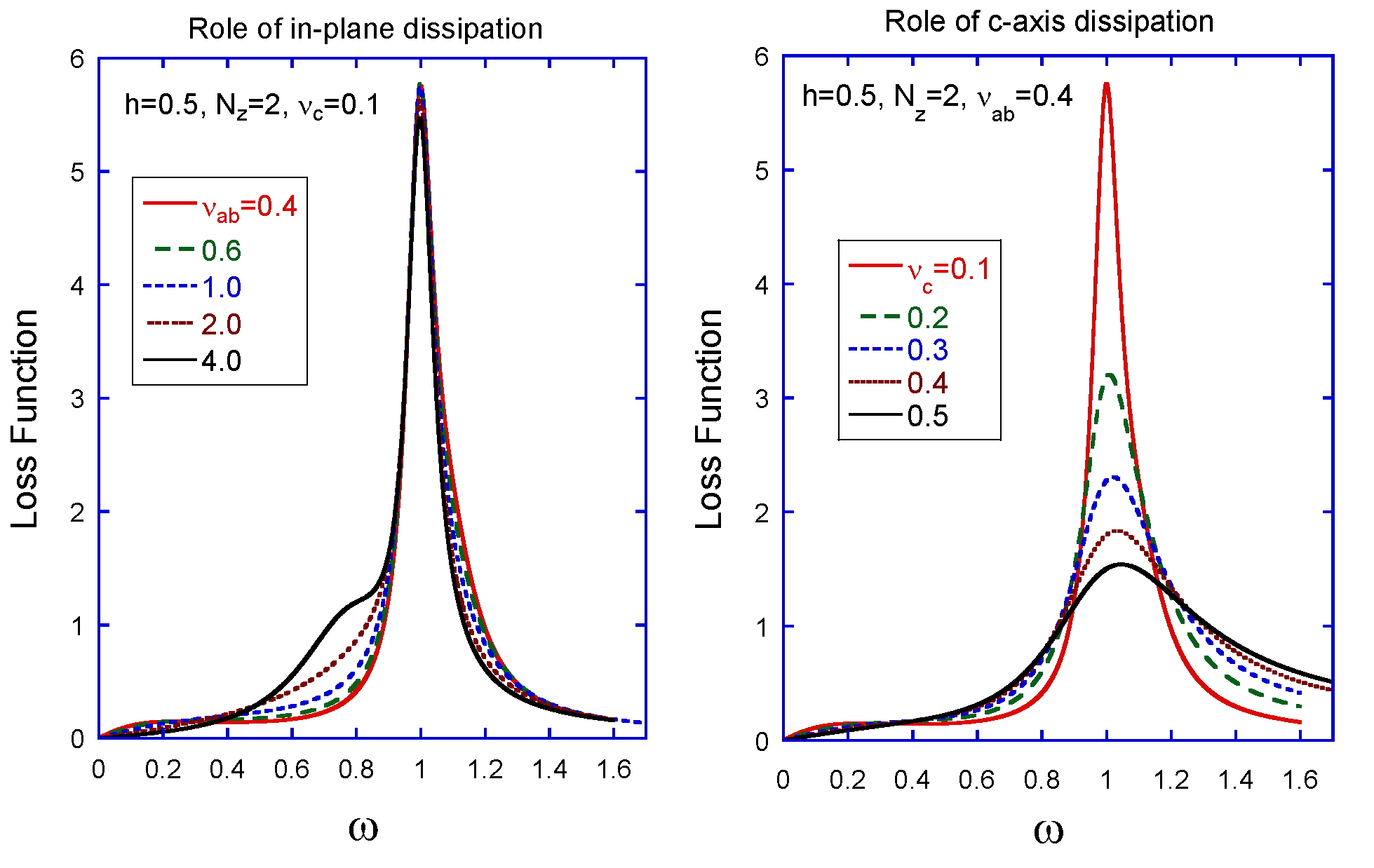
Figure 2: (Color online) Influence of the dissipation parameters on the loss-function shape in the dilute-lattice regime at $h=0.5$ and $N_{z}=2$. In-plane dissipation (left plot) does not influence much the JPR peak, but strongly influences the shape below the peak.

We start with the discussion of several general properties of the high-frequency response. To illustrate the roles of two different dissipation channels, we show in Fig. 2 series of the frequency dependencies of the loss function when only one damping constant is changed for fixed field $h=0.5$ and $N_{z}=2$ corresponding to a dilute lattice. We can see that the width of the JPR peak is mainly determined by the c-axis dissipation, while the in-plane dissipation has no visible influence on the loss function near the JPR peak. On the other hand, the in-plane dissipation strongly influences the shape of the loss function below the peak. In particular, at a very strong in-plane dissipation a peaklike feature appears below the JPR frequency which looks like an oscillation mode.

In Fig. 3 we compare the behavior of the numerically computed loss function at low frequencies with predictions of the vortex-oscillation model described in section IV. We can see that this model typically accurately describes the behavior at frequencies smaller then half the plasma frequency. At low dissipation, the loss function has an additional peak at small frequencies. This peak disappears with increasing dissipation. We have to emphasize that these plots are made for an ideal homogeneous system. In a real layered superconductor, pinning of the Josephson vortices by inhomogeneities will lead to the resonance peak at the pinning frequency.

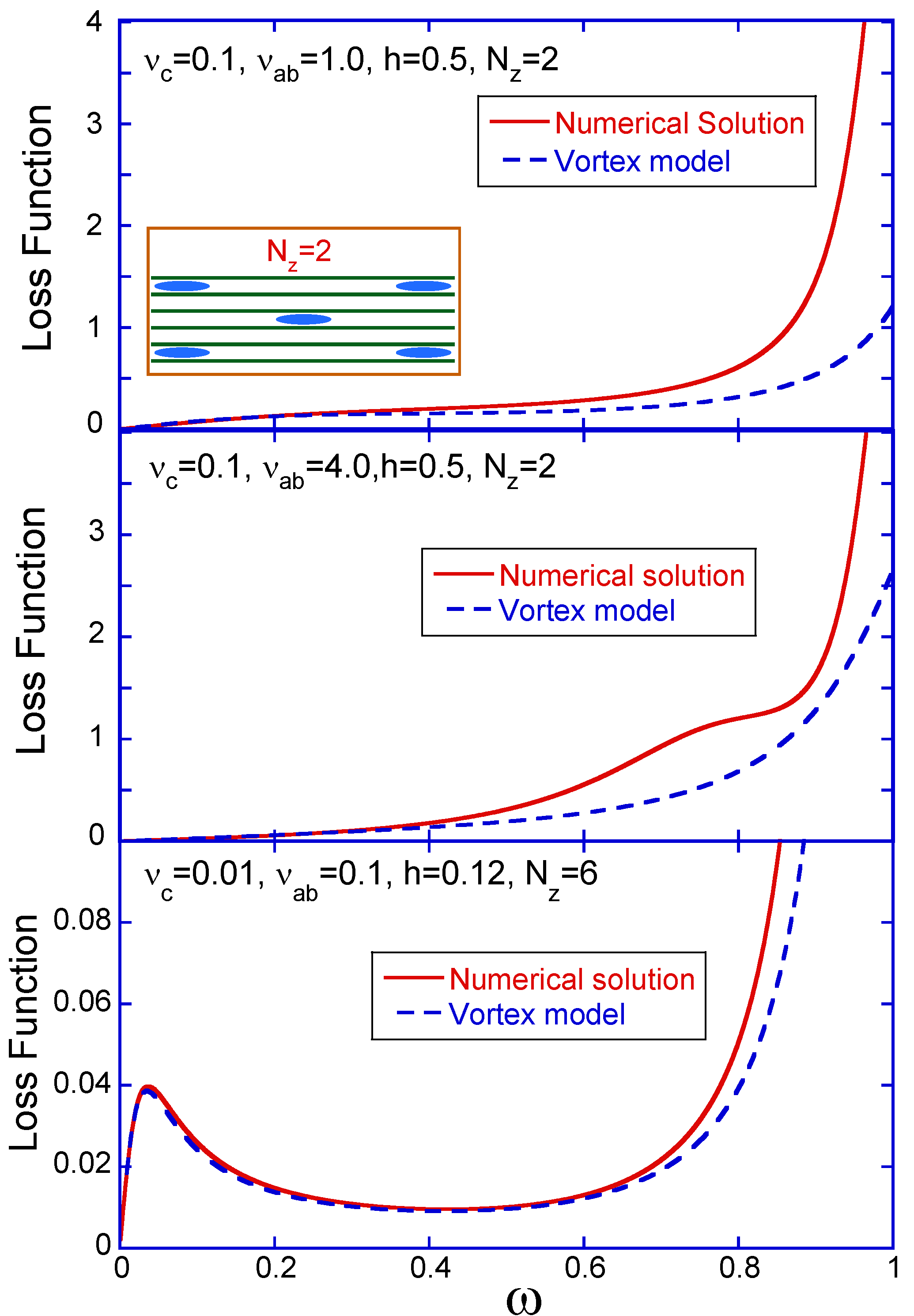
Figure 3: (Color online) Comparison between the vortex-oscillation model and exact numerical calculation for the loss function at several representative values of the dissipation parameters, field, and $N_{z}$ (shown in the plots). One can see that this model typically describes the high-frequency response roughly up to half of the plasma frequency. The inset in the upper plot illustrates the aligned lattice with $N_{z}=2$.

V.1 Small dissipation (BSCCO)

To illustrate a theoretically expected behavior of the high-frequency response in BSCCO, we made calculations with small dissipation parameters, typical for this compound, $\nu_{c}=0.01$ and $\nu_{ab}=0.1$. Figure 4 shows the evolution of the loss function with increasing magnetic field in the frequency range near the plasma resonance. For such small dissipation, the loss function at zero field has a very sharp peak at the plasma frequency. In the dilute-lattice regime at small fields, this peak decreases in amplitude and is displaced to slightly lower frequencies.

The most interesting feature of the dilute regime is the appearance of the satellite peaks in the high-frequency part. The strongest satellite is observed at $N_{z}=2$ near $h\sim 0.45$. A physical origin of these satellites is clear. In the vortex lattice state, the homogeneous oscillations are coupled to the plasma modes with the wave vectors set by the lattice. Therefore, the location of the satellites is determined by the plasma spectrum. For reference, we present the plasma frequencies at the reciprocal-lattice vectors in Appendix B. At small dissipations the shape of the loss function is not rigidly fixed by the value of the magnetic field, it is also sensitive to the lattice structure. This is illustrated in Fig. 5, where the loss function is plotted at fixed $h$ for two values of $N_{z}$, for which the lattice energies are close. One can see that the loss function is almost $N_{z}$ independent at frequencies below the JPR peak indicating that in this frequency range the vortices contribute independently to the response. However, above the peak the shape of the loss function is very sensitive to $N_{z}$. This means that the high-frequency response can potentially be used to probe the lattice structure.

In the dense-lattice limit, the plasma peak moves to a higher frequency and its intensity rapidly decreases, as predicted by the analytical theory in Section III. This behavior is also consistent with experiment KakeyaPRB05 . The transition to the dense lattice is very distinct. While for $N_{z}=2$ and $h=1$ the peak is still located very close to the zero-field JPR frequency and its amplitude is comparable with the zero-field peak, at very close field $h=1.4$ in the dense-lattice regime, $N_{z}=1$, the peak is noticeably shifted to a higher frequency, its amplitude considerably dropped, and the width increased.

An additional broad peak exists at low frequencies. Its intensity is much smaller than the JPR peak. The evolution of this peak with increasing magnetic field is shown in the inset of Fig. 4. One can see that the intensity of this peak monotonically increases with the magnetic field. This peak is well described by the vortex-oscillation model.

We did not find any intrinsic resonances in the loss functions at frequencies smaller than the JPR frequency, meaning that there are no modes coupled to homogeneous oscillations in this frequency range for a homogeneous superconductor.AntiphaseMode This suggests that the resonance feature observed in underdoped BSCCO at $\sim 0.5\omega_{p}$ in Ref. KakeyaPRB05, probably has an extrinsic origin, e.g., it may be caused by the pinning of the Josephson vortices.

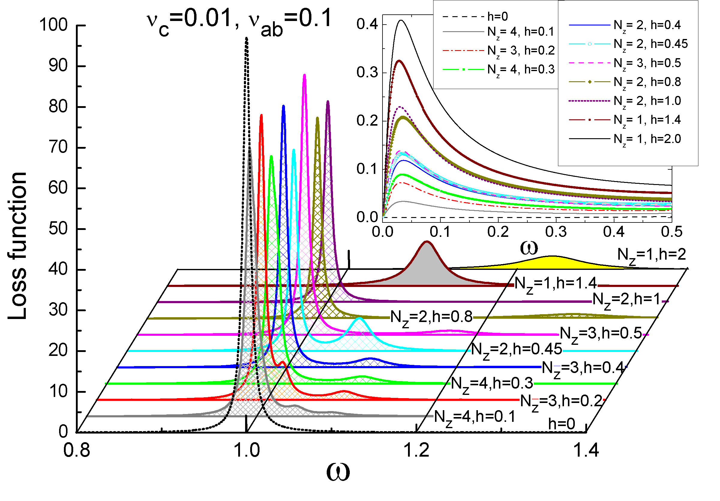
Figure 4: (Color online) Series of the frequency-dependent loss functions near JPR frequency at different fields for $\nu_{c}=0.01$ and $\nu_{ab}=0.1$. The inset shows the low-frequency region for the same set of parameters.

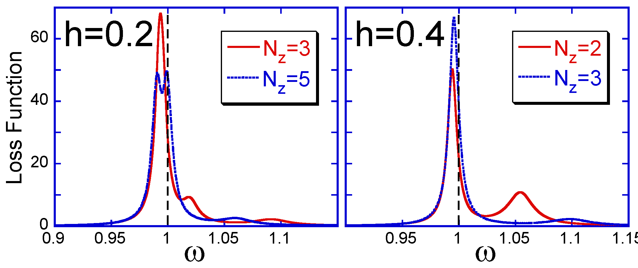
Figure 5: (Color online) Plots of the loss function at the same $h$ but with different $N_{z}$ for $\nu_{c}=0.01$ and $\nu_{ab}=0.1$. This figure illustrates the sensitivity of the loss-function shape to the vortex lattice structure (value of $N_{z}$) above the JPR peak.

V.2 Large dissipation (underdoped YBCO)

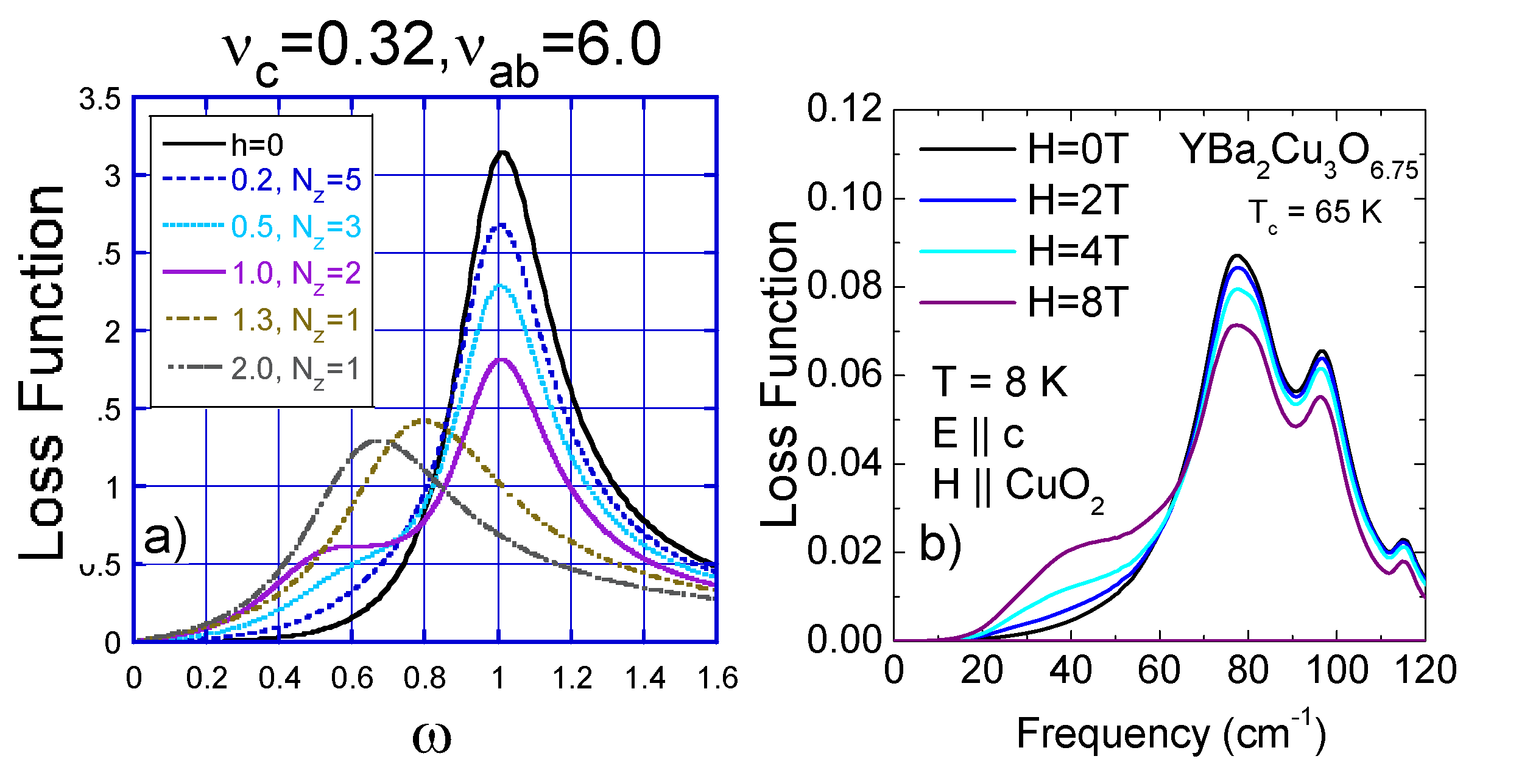
Figure 6: (Color online) (a)Series of the frequency-dependent loss functions at different fields for $\nu_{c}=0.32$ and $\nu_{ab}=6.0$. For comparison plot (b) shows the evolution of the loss function with increasing in-plane field for underdoped YBCO from Ref. LaForge, .

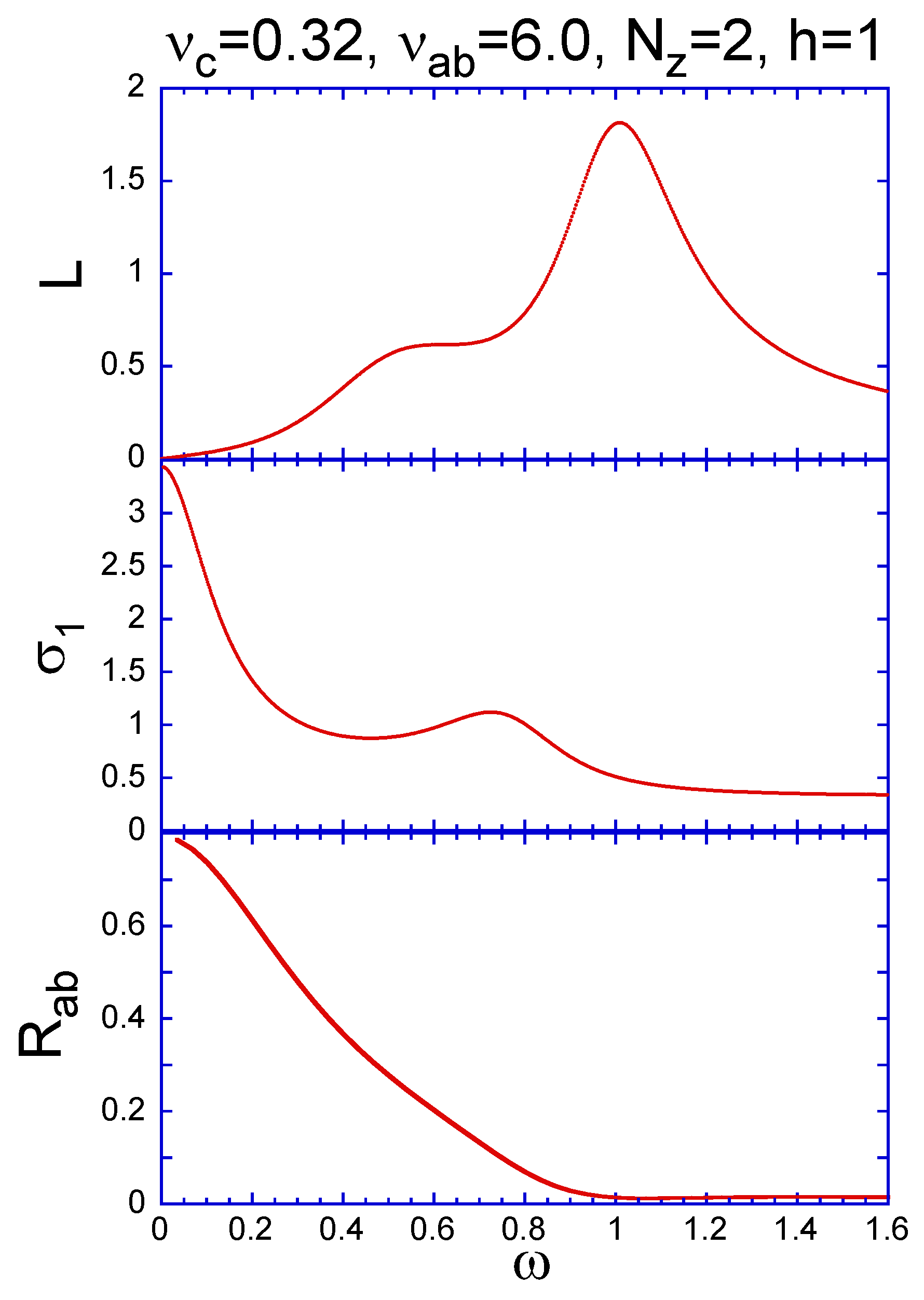
Figure 7: (Color online) The frequency dependences of the loss function, real part of conductivity, and relative contribution of in-plane dissipation (27) for the same damping parameters as in Fig. 6, $N_{z}=2$, and $h=1$. Rapid decreasing of in-plane inhomogeneity of the oscillations with increasing frequency can also be seen from the visualization of oscillating patterns of the local electric fields at different frequencies.Anim

In this subsection we discuss the high-frequency response of the Josephson vortex lattice in the case of large effective dissipation, which is realized, e.g., for the underdoped YBCO.KojimaJLTP03 ; LaForge Figure 6 shows the frequency dependences of the loss functions for the dissipation parameters $\nu_{c}=0.32$ and $\nu_{ab}=6.0$. For comparison, we also present the loss functions at different in-plane fields for an underdoped YBCO sample from Ref. LaForge, . One can see that two experimental features are well reproduced by the theory: decreasing intensity of the main peak with increasing field and the appearance of the satellite peak in the low-frequency part of the line. The origin of this satellite peak is distinctly different from the high-frequency satellites found for small dissipation. Figure 2 demonstrates that this peak only appears for sufficiently strong in-plane dissipations. As this peak is absent in the low-dissipation limit, it does not correspond to any specific mode of phase oscillations. It is caused by the decrease of the relative contribution of the in-plane dissipation channel with increasing frequency. To verify this interpretation, we plot in Fig. 7 the loss function for $N_{z}=2$ and $h=1$ together with the relative contribution of in-plane dissipation to losses, $R_{ab}=\sigma_{ab}\overline{E_{x}^{2}}/(\sigma_{c}\overline{E_{z}^{2}}+\sigma_{ab}\overline{E_{x}^{2}})$, which can be rewritten in reduced coordinates,

$$R_{ab}=\frac{\nu_{ab}\overline{\left|\partial\phi_{n}/\partial x\right|^{2}}}{\nu_{c}\left(1+\overline{|\phi_{n+1}-\phi_{n}|^{2}}\right)+\nu_{ab}\overline{\left|\partial\phi_{n}/\partial x\right|^{2}}}.$$ (27)

One can see that $R_{ab}$ decreases with increasing frequency and almost vanishes above the plasma resonance. The small-frequency peak roughly corresponds to the frequency where $R_{ab}$ drops to one half. The decrease of the in-plane dissipation also leads to the peak in the real part of the optical conductivity $\sigma_{1}$, also shown in Fig. 7. Note that the peak in $\sigma_{1}$ corresponds to the dip in the loss function.

At high fields, in the dense-lattice limit, only a single broad dissipation peak remains. In contrast to the low-dissipation case, this peak is displaced to lower frequencies with increasing magnetic field. This behavior is not verified experimentally yet, data are only available for field range $h\lesssim 1$.KojimaJLTP03 ; LaForge

VI Summary

In summary, we developed a comprehensive description of the high-frequency response of the Josephson vortex lattice in layered superconductors. We found the general relation (13) connecting the dynamic dielectric constant with the averages containing the static and oscillating phases. Analytical formulas for the dynamic dielectric constant and loss function were derived for the high-field regime and the vortex-oscillation regime at low frequencies. Numerically solving equations for the oscillating phases, we explored the evolution of the loss function with increasing magnetic field for the cases of weak dissipation describing BSCCO and strong dissipation describing underdoped YBCO. Several new features were found. The most interesting feature in the weak-dissipation case is the high-frequency satellites in the dilute-lattice regime, which appear due to the excitation of plasma modes at the wave vectors of the reciprocal lattice. In the strong-dissipation limit, we reproduced the additional peak in the loss function below the JPR peak experimentally observed in underdoped YBCO.LaForge ; KojimaJLTP03 We established that this peak appears due to the frequency dependence of the in-plane contribution to losses.

VII Acknowledgments

This work was motivated by illuminating discussions of experimental data with D. Basov, A. LaForge, and I. Kakeya. This work was supported by the U. S. DOE, Office of Science, under contract # DE-AC02-06CH11357.

Appendix A Josephson-vortex mass and viscosity

The viscosity of an isolated Josephson vortex has been considered in Refs. CoffeyClemJViscPRB90, and JVflux-flow, . In the case when the dissipation is caused both c-axis and in-plane quasiparticle transport, the viscosity coefficient is given by

$$\eta_{J} =\frac{1}{\gamma s^{2}}\left(\frac{\Phi_{0}}{2\pi c}\right)^{2}\left[C_{c}\sigma_{c}+C_{ab}\frac{\sigma_{ab}}{\gamma^{2}}\right],$$

$$=\frac{\varepsilon_{c}\omega_{p}\Phi_{0}^{2}}{\pi\left(4\pi cs\right)^{2}\gamma}\left[C_{c}\nu_{c}+C_{ab}\nu_{ab}\right],$$ (28)

where the numerical constants $C_{c}$ and $C_{ab}$ are determined by the phase distribution of an isolated Josephson vortex, $\phi_{n}^{(0)}$,

$$C_{c} =\sum_{n=-\infty}^{\infty}\int_{-\infty}^{\infty}du\left(\frac{\partial\left(\phi_{n+1}^{(0)}-\phi_{n}^{(0)}\right)}{\partial u}\right)^{2}\approx 9.0,$$

$$C_{ab} =\sum_{n=-\infty}^{\infty}\int_{-\infty}^{\infty}du\left(\frac{\partial^{2}\phi_{n}^{(0)}}{\partial u^{2}}\right)^{2}\approx 2.4.$$

The mass of the Josephson vortex has been considered in Ref. CoffeyClemVMassPRB92, . This mass is determined by the kinetic energy, $\mathcal{E}_{k}$, which for a moving Josephson vortex can be presented as

$$\mathcal{E}_{k} =\int d^{3}\mathbf{r}\frac{\varepsilon_{c}E_{z}^{2}}{8\pi}=s\sum_{n}\int d^{2}\mathbf{r}\frac{\varepsilon_{c}}{8\pi}\left(\frac{\Phi_{0}}{2\pi cs}\right)^{2}\dot{\theta}_{n}^{2}$$

$$=\frac{v^{2}}{2}s\sum_{n}\int d^{2}\mathbf{r}\frac{\varepsilon_{c}}{4\pi}\left(\frac{\Phi_{0}}{2\pi cs}\right)^{2}\left(\frac{d\theta_{n}^{(0)}}{dx}\right)^{2}.$$

For a slowly moving vortex with velocity $v$, the phase difference is determined by its static distribution, $\theta_{n}(\mathbf{r},t)=\theta_{n}^{(0)}(x-vt)$, and we obtain

$$\mathcal{E}_{k}=L_{y}\frac{v^{2}}{2}s\sum_{n}\int dx\frac{\varepsilon_{c}}{4\pi}\left(\frac{\Phi_{0}}{2\pi cs}\right)^{2}\left(\frac{d\theta_{n}^{(0)}}{dx}\right)^{2}.$$

As, by definition, $\mathcal{E}_{k}=L_{y}\rho_{J}v^{2}/2$, we obtain the following result for the linear vortex mass

$$\rho_{J} =\frac{\varepsilon\Phi_{0}^{2}}{\pi\left(4\pi c\right)^{2}s}\sum_{n=-\infty}^{\infty}\int_{-\infty}^{\infty}dx\left(\frac{d\theta_{n}}{dx}\right)^{2}$$

$$=\frac{C_{c}\varepsilon\Phi_{0}^{2}}{\pi\gamma\left(4\pi cs\right)^{2}}.$$ (29)

The reduced combination in the dynamic dielectric constant (25) can be represented as

$$\frac{1}{\rho_{J}\omega^{2}+i\eta_{J}\omega}\frac{B\Phi_{0}}{4\pi\lambda_{c}^{2}}=\frac{2\pi h}{C_{c}\left(\tilde{\omega}^{2}+i\nu_{c}\tilde{\omega}\right)+C_{ab}i\nu_{ab}\tilde{\omega}}.$$

Appendix B Plasma frequencies at reciprocal lattice vectors: Expected location of satellites

The satellite peaks are expected approximately at the plasma frequencies for the wave vectors of the reciprocal lattice. In the reduced coordinates, the plasma spectrum at the zero magnetic field and without the charging effects is given by

$$\omega_{p}^{2}(\mathbf{k},q)=1+\frac{k^{2}}{1/l^{2}+2(1-\cos q)}$$ (30)

where $\mathbf{k}$ and $q$ are the wave-vector components along and perpendicular to the layers respectively. The reciprocal vectors of the vortex lattice are given by

$$(k_{(n,m)},q_{(n,m)})=(2\pi n/a,2\pi(m-n/2)/N_{z}),$$

where $n$ and $m$ are the integer indices and $a$ is the vortex separation, $a=2\pi/hN_{z}$. Neglecting the small factor $1/l^{2}$, we obtain for the satellite frequencies

$$\omega_{s}^{2}(n,m)\approx 1+\frac{\left(hN_{z}n\right)^{2}/2}{1-\cos\left[2\pi\left(m-n/2\right)/N_{z}\right]}.$$ (31)

The most intense satellite is expected for the basic reciprocal vector with indices $(n,m)=(1,0)$

$$\omega_{s}^{2}(1,0)=1+\frac{\left(hN_{z}\right)^{2}/2}{1-\cos\left[\pi/N_{z}\right]}$$

In particular, for $N_{z}=2$, this gives $\omega_{s}^{2}(1,0)=1+2h^{2}$.

References

- (1) S. N. Artemenko and A. G. Kobel’kov, JETP Lett. 58, 445 (1993).
- (2) M. Tachiki, T. Koyama, and S. Takahashi, Phys. Rev. B 50, 7065 (1994).
- (3) L. N. Bulaevskii, M. P. Maley, and M. Tachiki, Phys. Rev. Lett. 74, 801 (1995).
- (4) R. Kleiner and P. Müller, Phys. Rev. B 49, 1327 (1994).
- (5) A. A. Yurgens, Supercond. Sci. Technol. 13, R85 (2000).
- (6) M. B. Gaifullin, Yuji Matsuda, N. Chikumoto, J. Shimoyama, K. Kishio, and R. Yoshizaki, Phys. Rev. Lett. 83, 3928 (1999).
- (7) S. V. Dordevic, S. Komiya, Y. Ando, Y. J. Wang, D. N. Basov, Phys. Rev. B 71, 054503 (2005).
- (8) O. K. C. Tsui, N. P. Ong, Y. Matsuda, Y. F. Yan, and J. B. Peterson, Phys. Rev. Lett., 73, 724 (1994); O.K. C. Tsui, N. P. Ong, and J. B. Peterson, Phys. Rev. Lett., 76, 819 (1996); N. P. Ong, S. P. Bayrakci, O. K. C. Tsui, K. Kishio, and S. Watauchi, Physica C 293, 20 (1997).
- (9) Y. Matsuda, M. B. Gaifullin, K. Kumagai, K. Kadowaki, and T. Mochiku, Phys. Rev. Lett. 75, 4512 (1995); Y. Matsuda, M. B. Gaifullin, K. Kumagai, M. Kosugi, and K. Hirata, Phys. Rev. Lett. 78, 1972 (1997); Y. Matsuda, M. B. Gaifullin, K. Kumagai, K. Kadowaki, T. Mochiku, and K. Hirata, Phys. Rev. B, 55, R8685 (1997); M. B. Gaifullin, Y. Matsuda, N. Chikumoto, J. Shimoyama, and K. Kishio, Phys. Rev. Lett. 84, 2945 (2000).
- (10) K. Kadowaki, I. Kakeya, M. B. Gaifullin, T. Mochiku, S. Takahashi,T. Koyama, and M. Tachiki Phys. Rev. B 56, 5617 (1997); I. Kakeya, K. Kindo, K. Kadowaki, S. Takahashi, and T. Mochiku, Phys. Rev. B 57, 3108 (1998).
- (11) T. Shibauchi, T. Nakano, M. Sato, T. Kisu, N. Kameda, N. Okuda, S. Ooi, and T. Tamegai, Phys. Rev. Lett. 83, 1010 (1999).
- (12) S. Colson, M. Konczykowski, M. B. Gaifullin, Yuji Matsuda, P. Gierłowski, M. Li, P. H. Kes, and C. J. van der Beek, Phys. Rev. Lett. 90, 137002 (2003); S. Colson, C. J. van der Beek, M. Konczykowski, M. B. Gaifullin, Y. Matsuda, P. Gierłowski, Ming Li, and P. H. Kes, Phys. Rev. B 69, 180510(R) (2004);
- (13) D. Dulić, S. J. Hak, D. van der Marel, W. N. Hardy, A. E. Koshelev, R. Liang, D. A. Bonn, and B. A. Willemsen, Phys. Rev. Lett. 86, 4660 (2001).
- (14) V. K. Thorsmølle, R. D. Averitt, M. P. Maley, M. F. Hundley, A. E. Koshelev, L. N. Bulaevskii, and A. J. Taylor, Phys. Rev. B 66, 012519 (2002); V. K. Thorsmølle, R. D. Averitt, T. Shibauchi, M. F. Hundley, and A. J. Taylor, Phys. Rev. Lett. 97, 237001 (2006).
- (15) L. N. Bulaevskii and J. R. Clem, Phys. Rev. B, 44, 10234 (1991).
- (16) A. E. Koshelev, Proceedings of FIMS/ITS-NS/CTC/PLASMA 2004, Tsukuba, Japan, Nov. 24-28, 2004, cond-mat/0602341 (unpublished).
- (17) Y. Nonomura and X. Hu, Phys. Rev. B 74, 024504 (2006).
- (18) J. U. Lee, J. E. Nordman, and G. Hohenwarter, Appl. Phys. Lett., 67, 1471 (1995); J. U. Lee , P. Guptasarma, D. Hornbaker, A. El-Kortas, D. Hinks, and K. E. Gray Appl. Phys. Lett., 71, 1412 (1997).
- (19) G. Hechtfischer, R. Kleiner, A. V. Ustinov, and P. Müller, Phys. Rev. Lett. 79, 1365 (1997); G. Hechtfischer, R. Kleiner, K. Schlenga, W. Walkenhorst, P. Müller, and H. L. Johnson, Phys. Rev. B, 55, 14638 (1997).
- (20) Yu. I. Latyshev, P. Monceau, and V. N. Pavlenko, Physica C 282-287, 387 (1997); Physica C 293, 174 (1997); Yu. I. Latyshev, M. B. Gaifullin, T. Yamashita, M. Machida, and Y. Matsuda, Phys. Rev. Lett., 87, 247007 (2001).
- (21) I. Kakeya, T. Wada, R. Nakamura, and K. Kadowaki, Phys. Rev. B 72, 014540 (2005).
- (22) A. D. LaForge, W. J. Padilla, K. S. Burch, Z. Q. Li, S. V. Dordevic, K. Segawa, Y. Ando, and D. N. Basov, arXiv:0705.0045 (unpublished)
- (23) K. M. Kojima, S. Uchida, Y. Fudamoto, and S. Tajima, Phys. Rev. Lett., 89, 247001 (2002); Journ. of Low Temp. Phys., 131, 775 (2003).
- (24) L. N. Bulaevskii, D. Domínguez, M. P. Maley, and A. R. Bishop, Phys. Rev. B 55, 8482 (1997).
- (25) T. Koyama, Phys. Rev. B 68, 224505 (2003).
- (26) L. N. Bulaevskii, M. Zamora, D. Baeriswyl, H. Beck, and J. R. Clem, Phys. Rev. B, 50, 12831 (1994); R. Kleiner, P. Müller, H. Kohlstedt, N. F. Pedersen, and S. Sakai, Phys. Rev. B, 50, 3942 (1994).
- (27) S. N. Artemenko and S. V. Remizov, JETP Lett. 66, 853 (1997).
- (28) A. E. Koshelev and I. Aranson, Phys. Rev. B, 64, 174508 (2001).
- (29) T. Koyama, and M. Tachiki, Phys. Rev. B 54, 16183 (1996); S. N. Artemenko and A. G. Kobel’kov, Phys. Rev. Lett. 78, 3551 (1997).
- (30) M. W. Coffey and John R. Clem, Phys. Rev. Lett. 67, 386 (1991); Phys. Rev. B 46, 11757 (1992).
- (31) Yu. I. Latyshev, A. E. Koshelev, and L. N. Bulaevskii, Phys. Rev. B 68, 134504 (2003).
- (32) D. A. Bonn, P. Dosanjh, R. Liang, and W. N. Hardy, Phys. Rev. Lett. 68, 2390 (1992); D. A. Bonn, S. Kamal, K. Zhang, R. Liang, D. J. Baar, E. Klein, and W. N. Hardy, Phys. Rev. B 50, 4051 (1994); A. Hosseini, R. Harris, S. Kamal, P. Dosanjh, J. Preston, R. Liang, W. N. Hardy, and D. A. Bonn, Phys. Rev. B 60, 1349 (1999).
- (33) Shih-Fu Lee, D. C. Morgan, R. J. Ormeno, D. M. Broun, R. A. Doyle, J. R. Waldram, and K. Kadowaki Phys. Rev. Lett. 77, 735 (1996); H. Kitano, T. Hanaguri, Y. Tsuchiya, K. Iwaya, R. Abiru, and A. Maeda J. Low Temp. Phys. 117, 1241 (1999).
- (34) M. W. Coffey and J. R. Clem, Phys. Rev. B 44, 6903 (1991)
- (35) J. R. Clem and M. W. Coffey, Phys. Rev. B 42, 6209 (1990)
- (36) A. E. Koshelev, Phys. Rev. B 62, R3616 (2000).
- (37) Analyzing modes of the dense triangular lattice, Koyama KoyamaPRB03 found the mode whose behavior strongly resembles the behavior of the experimental low-frequency peak in Ref. KakeyaPRB05, . However, this mode is the antiphase mode in which the phases oscillate with the phase shift in neghboring layers. At high fields the frequency of this mode can be computed analytically, . As the average oscillating phase is zero in this mode, it does not contribute to the response to the homogeneous-in-space oscillating electric field in a homogeneous superconductor. Coupling of this mode to homogeneous oscillations can be mediated, e. g., by correlated disorder.
- (38) Animations of oscillating patterns of local electric field at different frequencies for , , , and can be found at http://mti.msd.anl.gov/homepages/koshelev/projects/JPRinJVL/Nz2vc0_32vab6_0Anim.htm.