A New Measure of Fine Tuning
Peter Athron and D.J. Miller
Department of Physics and Astronomy, University of Glasgow,
Glasgow G12 8QQ, United Kingdom
Abstract
The solution to fine tuning is one of the principal motivations for Beyond the Standard Model (BSM) Studies. However constraints on new physics indicate that many of these BSM models are also fine tuned (although to a much lesser extent). To compare these BSM models it is essential that we have a reliable, quantitative measure of tuning. We review the measures of tuning used in the literature and propose an alternative measure. We apply this measure to several toy models and the Minimal Supersymmetric Standard Model.
I Introduction
Fine tuning appears in many areas of particle physics and cosmology, such as the Standard Model (SM) Hierarchy Problem and the Cosmological Constant Problem. These problems imply that the the universe we live in is a very atypical scenario of the theories we use to describe it. The contortion required to reproduce observation makes such theories seem unnatural, motivating many studies of Beyond the Standard Model (BSM) physics.
However many of the models constructed to solve fine tuning, also exhibit some degree of tuning themselves. In the absence of data, while we await the LHC, naturalness is used to compare models and judge their viability. Great importance has been attached to small differences in the levels of tuning when comparing models, so it is important that naturalness and fine tuning are rigorously understood and measured accurately.
For example the Hierarchy Problem is one of the fundamental motivations of low energy supersymmetry (SUSY) (for a review see Ref.[1]). If the SM is an effective theory, valid up to the Planck scale, then the inclusion of supersymmetric partners for every SM particle leads to the cancellation of quadratic divergences in the loop corrections to the Higgs mass. This removes the need for fine tuning of between the tree-level mass parameter and the Planck Mass, allowing the Higgs boson to be naturally light.
Unfortunately current limits on superpartner masses may imply fine tuning in the most studied model, the Minimal Supersymmetric Standard Model (MSSM). The minimisation of the Higgs potential sets the square of the boson mass, , in terms of the supersymmetry breaking scales. In the MSSM the tree-level expression for this is,
| (1) |
where is the ratio of vacuum expectation values, the bilinear Higgs superpotential parameter, and and are the up and down type Higgs scalar masses respectively.
Lower bounds on the masses of the supersymmetric particles and the Higgs translate to lower bounds on the parameters appearing on the right hand side of Eq. (1). If, for example, one of the parameters is TeV, then to cancel this contribution and give GeV [2], another parameter (or combination of parameters) would have to be tuned to the order of one part in a hundred.
Including loop corrections to Eq. (1) and examining the experimental constraints, one finds that the largest term is from corrections involving the heaviest stop. This can be written as [3],
| (2) |
where is the high scale at which the soft stop masses, and , are generated from the supersymmetry breaking mechanism and is the top Yukawa coupling. A heavy physical stop mass ( GeV) is needed to provide radiative corrections to the light CP even Higgs mass, of the form,
| (3) |
which are large enough to evade the LEP constraints on it’s mass ( GeV). So the Little Hierarchy Problem is really about the tension between the masses of the boson, the heaviest stop squark and the light Higgs.
The desire to solve this “Little Hierarchy Problem” has motivated a
flood of activity in the construction of supersymmetric models
[?–?]. There
is also increased interest in studying alternative solutions to the SM
Hierarchy problem [?–?]. In
addition to ensuring such models satisfy phenomenological constraints
it is essential that the naturalness is examined using a reliable,
quantitative measure of tuning.
In Ref.[14] Barbieri and Giudice use a measure of tuning, originally proposed in Ref.[15], for an observable, , with respect to a parameter, ,
| (4) |
A large value of implies that a small change in the parameter results in a large change in the observable, so the parameters must be carefully “tuned” to the observed value. Since there is one per parameter, they define the largest of these values to be the tuning for that point,
| (5) |
They then make the aesthetic choice that a tuning, is fine tuned.
This measure has been used extensively in the literature to quantify tuning in the MSSM [?–?] and to examine tuning in other models and theories e.g. [3],[?–?]. However other measures have also been proposed and used in the literature.
Motivated by global sensitivity, which will be discussed in the next section, Anderson and Castano [?–?] propose that tuning should be measured with,
| (6) |
where they choose the “average” sensitivity, , not to be the mean, but instead defined by,
| (7) |
where f(p) is the probability distribution of parameter . Individual are combined in the same manner as the individual were,
| (8) |
There is some dispute within the literature as to whether or not Eq. (5) is the best way of choosing a final tuning value from the set . In [11],[?–?] the individual are be combined as if uncorrelated,
| (9) |
Several other measures have been proposed
[?–?], but
will not be discussed here.
In Section II we detail some limitations of the traditional measure of tuning, , used for this Little Hierarchy Problem. We then describe our fundamental notion of tuning, and how this principle can be applied to construct quantitative measures of tuning in Section III. This leads us to present a new tuning measure in Section IV, which is also a generalisation of the traditional measure that overcomes the limitations outlined earlier. This measure is applied to several toy models in Section V to demonstrate how it works and compare the results it produces with those from other measures. Finally in Section VI we apply our measure to the Little Hierarchy Problem for a selection of Minimal SUperGRAvity (MSUGRA) inspired points.
II Limitations of the Traditional Measure
Despite the wide use of it has several limitations which may obscure the true picture of tuning:
-
•
variations in each parameter are considered separately;
-
•
only one observable is considered in the tuning measure, but there may be tunings in several observables;
-
•
it does not take account of global sensitivity;
-
•
only infinitesimal variations in the parameters are considered;
-
•
there is an implicit assumption that the parameters come from uniform probability distributions.
Tuning is really concerned with how the parameters are combined to produce an unnatural result. If one measures tunings for each parameter individually, there is no clear guide how to combine these tunings to quantify how unnatural this cancellation is. This has led to two alternative approaches in the literature, Eq. (5) and Eq. (9); the only way to determine if either or combines sensitivities correctly is to compare them with a generalisation of that varies all of the parameters simultaneously.
Secondly, some theories may contain significant tunings in more than one observable. We want to know how can these tunings be combined to provide a single measure. For example it is reported in Refs.[44, 45], and more recently in Refs.[46, 47], that the MSSM also requires tuning in the relic density of the dark matter (). To measure the tuning for some particular set, , of these observables we should determine how atypical predictions like are in the theory. There are four classes of scenario which are significant: the first where both and are similar to their value in ; two more classes where only one of or is similar to it’s value in ; one with neither observable similar to . Tunings in these two observables should be combined in a manner which measures how atypical scenarios in the first class are, without double counting scenarios which appear in the final class. Only a tuning measure which considers the observables simultaneously can achieve this.
A third problem, first mentioned by Anderson and Castano [32] is that the traditional measure picks up global sensitivity as well as true tuning. is really a measure of sensitivity. Consider the simple mapping , where . Applying the traditional measure to gives . Since is independent of , we follow the example of [32] and term this global sensitivity. Since for all , there is no relative sensitivity between points in the parameter space.
If we use as our tuning measure then appears fine tuned throughout the entire parameter space. This contrasts with our fundamental notion of tuning being a measure of how atypical a scenario is. A true measure of tuning should only be greater than one when there is relative sensitivity between different points in the parameter space.
Another concern is that only considers infinitesimal variations in the parameters. Since MSSM observables are complicated functions of many parameters, it is reasonable to expect some complicated distribution of the observables about that parameter space. There may be locations where some observables are stable (unstable) locally, but unstable (stable) over finite variations.
Finally, there is also an implicit assumption that all values of the parameters in the effective softly broken Lagrangian are equally likely. However they have been written down in ignorance of the high-scale theory, and may not match the parameters in, for example, the Grand Unified Theory (GUT) Lagrangian, . Any non-trivial relation between these different sets of parameters may alleviate or exacerbate the fine tuning problem.
While some of the alternative measures in the literature are motivated by one of these issues, no proposed measure fully addresses all of them.
III Constructing Tuning Measures
A physical theory is fine tuned when generic scenarios of the theory predict very different physics to that which is observed. For the theory to agree with observation the parameters must be adjusted very carefully to lie in an extremely narrow range of values. Insisting that the physics described by the theory is similar to that observed, shrinks the acceptable volume of parameter space. When in this tiny volume even small adjustments to the parameters will dramatically change the physics predicted, so fine tuning may also be characterised by instability. It is this instability which the traditional measure is exploiting.
Instead we wish to construct a tuning measure which determines how rare or atypical certain physical scenarios are. The most direct way to do this is to compare the volume of parameter space, , that is similar to some given scenario with the typical volume, , of parameter space formed by scenarios which are similar to each other.
If all the parameters are drawn from a uniform probability distribution then the probability of obtaining a scenario in is, , where is the volume of parameter space formed by all possible parameter choices. Similarly gives the probability of obtaining a scenario in volume . We may then define tuning as , to quantify the relative improbability of scenarios similar to our given scenario in comparison to the typical probability.
To place this within a quantitative framework we must define what we mean by “similar” and “typical”. This will be dealt with later. First, though, consider the toy example presented in Fig. I,
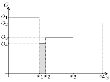
showing an observable, , which depends on a parameter, . Here there are four clearly distinct groups of observable scenario and “similar” can be replaced with equal. Given one of these groups of scenarios, , the volume is the length (one dimensional volume) of parameter space with . For example, for we have . Next we must define our “typical” volume, formed by these distinct groups of scenarios. In this simple example an obvious choice is to define as the mean volume (length) of parameter space formed by scenarios in the same group. So . The tuning required to get is then , which conforms to our intuitive expectation.
In more realistic examples the definitions of “similar” and “typical” will not be so trivial. The definitions must be chosen to fit the type of problem one is considering. In the simple example given above the problem was that scenarios where occupied a smaller proportion of the parameter space than other values, .
In hierarchy problems the concern is that one (or more) observable is much smaller than another observable, despite depending on common parameters. The requirement that one observable is large forces the theory into a region of parameter space where generic points also predict a large value for the second observable(s).
So “similar” must be related to the size of the observables. For example, one might consider “similar” to observable to mean observables “of the same order”as . A sensible definition of is then the volume of parameter space where , for all observables . However it is not clear that this is more appropriate than some other choice such as . So generally can be defined by a class of parameter space volumes formed from dimensionless variations in the observables . Different values of and quantify different definitions of “similar” and are therefore different fine-tuning questions. In comparison, the one dimensional measure is a ratio of infinitesimal lengths, so implicitly adopts the choice . One can imagine cases where this would be a bad choice (e.g. an observable which oscillates quickly when the parameter is varied), so care must be taken to choose and sensibly (i.e. ask the correct question).
When a large hierarchy between observables requires a large cancellation between parameters, as in the traditional hierarchy problem, the region of parameter space which can provide the correct observables (the volume ) is much smaller than one would expect (i.e. it is “fine-tuned”). We must compare this volume with the “typical volume” of parameter space, , that one would expect if no fine-tuning were present. The remaining question is then, how do we define this “typical volume”?
One might suggest that this typical volume should be the average of volumes throughout the whole parameter space, . However, the measure would then depend only on how far parameters are from some hypothesised upper limits on their values. For example, an observable which depends on a parameter according to will display fine-tuning for small values of if one chooses the maximum possible value of to be large, even though there is no cancellation present. This is not the ‘fine-tuning’ we are trying to probe; we want to gain insight into the unnatural cancellation between parameters, so must be anchored to the specific parameter point to be tested.
We can do this by adopting the same notion of “similar” that we used to define . We introduce a volume which is formed from dimensionless variations in the parameters. A comparison of at different points in the parameter space, provides a test of whether ’s variation is due to a simple scaling with the parameters (as described above for ), or due to some “unnatural” effect such as fine-tuning. Consequently one should compare with its average value over the entire space, . Reverting to our previous terminology, the “typical” volume which one would have expected to form from dimensionless variations in the parameters about , is
| (10) |
IV A New Measure
Following the above discussion and motivated by the limitations of the traditional measure, we propose a new measure of tuning.
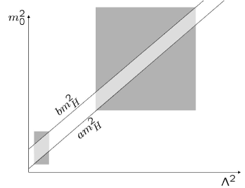
We define two volumes in parameter space for every point . Let be the volume of dimensionless variations in the parameters over some arbitrary range , about point , i.e. the volume formed by imposing . Similarly let be the volume in which dimensionless variations of the observables fall into the same range , i.e. the volume constrained by . Volumes and are illustrated for a two dimensional example in Fig. II.
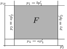
We define an unnormalised measure of tuning with,
| (11) |
This is sufficient for comparing different regions of parameter space within a given model as the normalisation factor will be common. To compare tuning in different models we need to include normalisation,
| (12) |
with,
| (13) |
Notice that this measure does not depend on experimental constraints. In naturalness problems such constraints should only rule out the point, , around which we make variations to test fine tuning. If is not experimentally excluded, we should not impose experimental constraints on nearby points used to probe fine tuning. Fine tuning quantifies how unnatural a region of parameter space is and this is a feature of the theory, not our experimental knowledge.
quantifies the restriction on parameter space. This
is more in touch with our intuitive notion of tuning than the
stability of the observable. Notice that with only one or two
parameters and no global sensitivity, also describes
restriction of parameter space and yields the same results as our new
measure. However it is important to recognise that ’s
ability to do this leads to its utility as a tuning measure
there. Equally its failure to do so in many dimensions demonstrates
its limitation.
Consider fine tuning for a single observable which depends on more than one parameter, Even though the true tuning for any physical scenario should be described using all available observables, it is often useful to define individual tunings for each observable separately. However, in this case, the volume is unbounded, since a single observable can only constrain one combination of parameters.
To resolve this difficulty one must either reduce the number of parameters to one or introduce some other bounds on . The former reintroduces the problem of combining tunings for individual parameters and a better procedure is to restrict to be within . Here we are trying to pick up how much of the restriction in parameter space is due to this particular observable. The assumption is made that if all other observables were natural then they would restrict no more than does. Therefore we define to be the volume restricted by and . Tuning is then defined by,
| (14) |
This definition is applied to obtain individual tunings in the MSSM in
Section VI.
Like and ,
depends upon the choice of parameterisation. Since tuning is about the
restriction of the parameter space this seems unavoidable. To examine
different choices of parametrisation one must redefine volumes and
in terms of the new parameters and normalise the tuning by taking
the average over the new parameter space.
Since much of the motivation behind developing this measure was to generalise so that many parameters and many observables are considered simultaneously, it is interesting to look at how the two measures are related.
Consider a theory with one observable, which has a linear dependence on a single parameter, , with the value of that parameter being drawn from a uniform probability distribution. At the parameter point , notice that, , while we can see and , so,
| (15) |
Similarly Anderson and Castano’s measure may be written as,
| (16) |
Now notice that , so,
| (17) |
V Toy Models
We now compare some of the tuning measures for various toy models and discuss the implications. In each of these examples we will assume a uniform probability distribution for the parameters.
Table 1 compares the analytical results of
various tuning measures for the simple models with only one parameter
and one observable. With only one parameter it is trivially the case
that , so it is not included.
| Toy SM | ||||
|---|---|---|---|---|
| Proton Mass |
In the first row of Table 1 are the results for a toy version of the Standard Model Hierarchy Problem, where we know the tuning is enormous. Here there is only one observable, the physical Higgs mass, . At one loop we write,
| (18) |
and treat only the bare mass squared, as a parameter. , the Ultra-Violet cutoff, is taken to be the Planck Mass or some other fixed scale, while is a positive constant.
Our measure was obtained by simply varying the tree-level mass parameter over the arbitrary range and applying the same dimensionless variations to the observable. This gives and , leading to the result for shown. Notice that the arbitrary range has fallen out of the result and it matches that obtained using the traditional measure, as shown earlier for all linear functions.
We also determine , and . In both cases this introduces a dependence on the allowed range of in the theory, so we specify , and present results where , though similar results can be obtained for other scenarios. These bounds give the total allowed range of the parameter in this model and should not be confused with the range of dimensionless variations which appears in the definition of . If we take the range of variation to be large, , then . Alternatively, if we choose a very narrow range of variation about , where , then is very small.
This is intuitively reasonable. Imagine some compelling theoretical reason for the bare mass to be constrained close to the cutoff, e.g. . In light of this, the case for new physics at low energies would be dramatically weakened. Indeed it is precisely because there is no such compelling reason that we worry about the hierarchy problem and look to BSM physics such as supersymmetry to explain how we can have .
Now let us compare this with the result for . and are the extremum values of ,
dictated by the extremum values of . Notice that as we have and , so . However a
fundamental difference between our measure and is
that the latter will give a large tuning for any . If the upper
bound is chosen such that, , then even a Higgs
mass of will appear fine tuned. This measure is not
sensitive to the unnatural cancellation which causes our concern.
Instead it is sensitive to the fact that large values of take
up a much larger volume of parameter space than small values of
. This would be true even if the Higgs mass was described by
, with no unnatural cancellation.
Also shown in Table 1 are the results for the
simple functions and . Earlier we showed
there was no relative sensitivity in . While
and can be large despite the absence of relative
sensitivity, our measure, , is exactly unity for all
. Anderson and Castano’s measure does remove the global
sensitivity, but their tuning criterion prefers the observable to be
as large as possible. For , while there is relative sensitivity
between different values of , the constant factor makes
for all . For
the situation is similar, with for all , where . In
the effect of is removed and though tuning still
increases with , this is now contextualised by comparing it to
. It is interesting that our measure considers
to have consistently no tuning (), whereas it is
for that for all .
The original illustration of global sensitivity presented by Anderson and Castano in Ref.[32] was for the proton mass. The proton can be much lighter than the Planck Mass without fine tuning because the renormalisation group equations (RGE) lead to only a logarithmic dependence on high scale quantities. However, by using the one loop RGE for the QCD coupling, , and equating the proton mass to the QCD scale111For details see [32]
| (19) |
where is the strong gauge coupling evaluated at the Planck scale, , and C is a positive constant. As they demonstrated, this gives .
The analytical results for tuning in the mass of the proton, using
Eq. (19), are shown in the final row of Table
1. Notice that while the unnormalised tunings
are both , and are small.
The latter has been determined only approximately in the limit where
and for all
, where .
In these one parameter examples the need for a normalised tuning measure is apparent. However diverges significantly from our new measure, which in many of these simple one dimensional models is equivalent to normalising the traditional measure with it’s mean value.
It is also interesting that even after accounting for global
sensitivity some of these one dimensional functions may still show
some small degree of tuning. This opens up the possibility that
changing the parameterisation of the effective low energy theory might
exacerbate or alleviate the tuning problem. Finding choices of
parametrisation which reduce tuning could allow us to select high
scale theories which are preferential in terms of naturalness. This point
has not appeared in the literature and merits investigation. However
we do not address this here but leave it for a future study.
Now we consider models with more than one parameter. In these cases diverges from and we must compare each of these with .
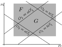
First we return to the SM hierarchy problem, but this time treat as a function of two parameters, and . In the one dimensional example the tension between the weakness of gravitation (the large Planck Mass) and a light Higgs mass was examined indirectly by choosing the Planck mass to be a fixed constant in theory. We now take a more direct route with two observables and (“observed” to be large due to the weakness of gravitation), predicted from the parameters with,
| (20) |
We are still predicting from Eq. (18) and have not split up any of the terms to introduce new cancellations, so we expect to simply reproduce the same result for as we obtained in the one parameter toy SM model. However, the method applied provides a simple illustration of how our measure works with more than one parameter. We have a two dimensional parameter space, so allowing the parameters to vary about some point over the dimensionless interval defines an area, , in this space. Clearly the bounds from dimensionless variations in are the same as those from , while the bounds from dimensionless variations in introduce two new lines in the parameter space.
This is shown in Fig. III for two different points. In the first point, the values of the parameters are of the same order as the observable, , because we have chosen a small value of . So is not much smaller than . For the other point , resulting in an much larger than and fine tuning. Of course neither of these points are representative of the weakness of gravitation we observe. A point with and , would have to such an extent that a graphical illustration is not possible.
In general the areas are, and so,
| (21) |
In this simple case we find the same result as the traditional measure. Combining and as if they are uncorrelated, gives,
| (22) |
With and both , i.e. fine tuned
scenarios, this gives us . While our measure does not deviate from
in this simple example, models with additional
parameters allow the observable to be obtained from cancellation of
more than two terms, complicating the fine tuning picture.
We now look at a model with four observables, , , , , and three parameters, , , , described by,
| (23) |
| (24) |
For a point , in the three dimensional parameter space, the traditional measure gives (no sum over is implied), so,
| (25) |
To apply our tuning measure in the three dimensional case we must determine volumes and . For a point, , with we have,
| (26) | |||||
| (27) |
where the latter uses and is the usual Heaviside step function. Integrating Eq. (26) over all three gives the volume,
| (28) |
and similarly Eq. (27) gives,
| (29) | |||||
We find that the analytical expressions for tuning in this model
depend on the mass hierarchy of , and .
For we find,
| (30) |
For we find:
| (31) |
For and :
| (32) |
For and :
| (33) |
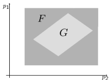
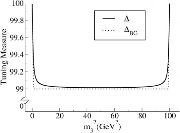
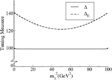
Notice that these results do not match , but in three dimensions at least is a much better approximation, as is shown in Fig. IV.
However, as we have seen, in moving from two parameters to three parameters these discrepancies appeared, increasing the number of parameters further will increase the divergences between the measures.
VI Fine Tuning in the MSSM
The analytical methods described above become increasingly complicated to apply as the number of parameters and observables are increased. For such situations we have also developed a numerical procedure which can be applied to produce approximate results for tuning. Since the MSSM contains many parameters and many observables we chose to apply our numerical approach here.
We take random dimensionless fluctuations about an MSSM point at the GUT scale, , to give new points . These are passed to a modified version of Softsusy 2.0.5[48]. Each random point is run down from the GUT scale until Electroweak Symmetry is broken. An iterative procedure is used to predict and then all the sparticle and Higgs masses are determined. For a theoretical discussion, see Ref.[49].
As before is the volume formed by dimensionless variations in the parameters. is the sub-volume of additionally restricted by dimensionless variations in the single observable , . As usual is the volume restricted by , for each observable, , where is the set of masses predicted in Softsusy. For every a count, , is kept of how often the point lies in the volume as well as an overall count, , kept of how many points are in . Tuning is then measured according to,
| (34) |
for individual observables and
| (35) |
for the overall tuning at that point.
Before describing the results two comments on this approach should be made. Firstly when using Softsusy to predict the masses for the random points, sometimes problems are encountered. We may have a tachyon, the Higgs potential unbounded from below, or non-perturbativity. Such points don’t belong in volume as they will give dramatically different physics. However it is unclear which volumes, , the point lies in. Such points never register as hits in any of the and this may artificially inflate the individual tunings, including . Keeping the range small reduces the number of problem points. Therefore we chose and for our dimensionless variations.
Secondly, since we are measuring tuning for individual points
numerically and cover only a small sample of points, it is not
possible to obtain mean values of and the
as we haven’t sampled the entire space. When
simply comparing how the tuning varies about the parameter space the
normalisation factor is not needed. However to compare the tuning
between different observables as well as to compare with different
models some form of normalisation is essential.
We considered points on the Constrained Minimal Supersymmetric Standard Model (CMSSM) benchmark slope222Such benchmark slopes and points, known as Snowmass Points and slopes (SPS)[50] are chosen by consensus as representing qualitatively different MSSM scenarios and are very useful for comparison with other work. , SPS 1a [50]. This slope is defined by,
| (36) |
where is the common scalar mass, the common gaugino mass (both at the GUT scale) and is the undetermined sign of , the magnitude being determined from a loop corrected, inverted form of Eq. (1) with set to it’s observed value. is the common multiplicative factor which relates the supersymmetry breaking matrices of trilinear mass couplings to their corresponding Yukawa matrix, e.g. .
The parameters we vary simultaneously are the set333Note that since points on the SPS 1a slope have set by , our tuning measure is not sensitive to the -problem. However for our random variation about the SPS 1a points we do treat as a parameter because we are predicting from the parameters, not fixing it to it’s observed value. , where is the soft bilinear Higgs mixing parameter and are the Yukawa couplings of the top, bottom and tau respectively. The gauge couplings are not included as parameters. Doing so would introduce excessive global sensitivity, increasing the statistics needed to keep the errors under control.
First we applied our tuning measure to the observable for 13 points on the SPS 1a slope. Moving along this slope in is an increase in the overall supersymmetry breaking scale, since the magnitude of every soft breaking term is increasing. We have plotted the results of this investigation in Figure V.
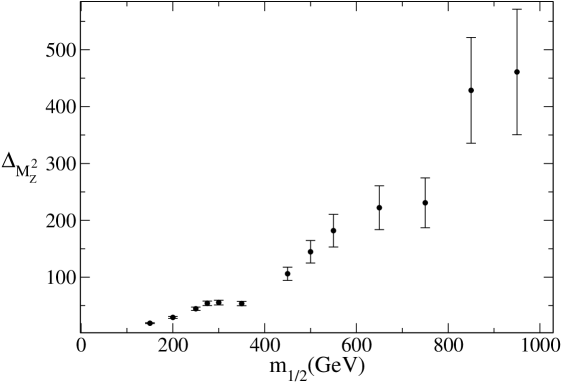
As expected there is a clear increase in tuning as the supersymmetry breaking scale is raised. The statistical error also increases with the tuning, making the numerical approach most difficult to apply when the tuning is large. However precise determinations of tuning are only relevant for moderate and low tunings. With tunings greater than , precise values are not required.
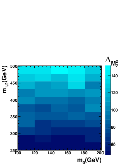
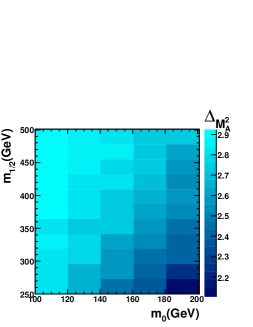
Due to the difficulty in this approach for measuring large tunings we looked in more detail at points expected to have moderate tuning. We chose a grid of points with,
| (37) |
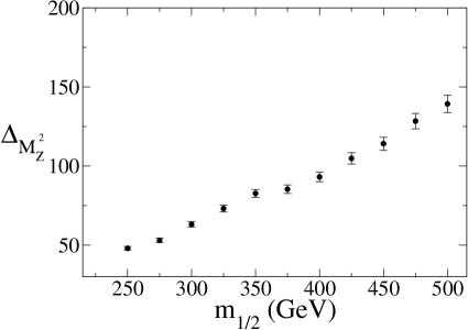
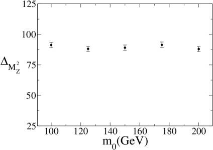
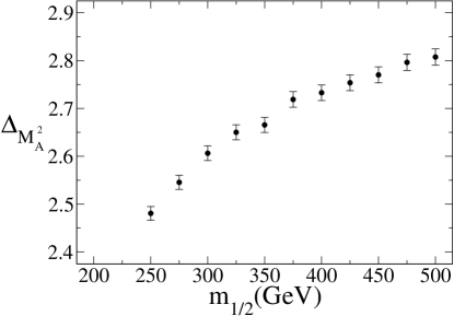
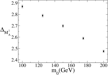
Shown in Fig. VI (top) is a plot of over this grid of points. While the errors are still significant () there is a clear trend of tuning increasing with . Also shown (bottom left) is averaged over the five different values of . This substantially reduces the errors giving a much more stable picture of tuning increasing linearly with . Similarly , averaged over the eleven different values of , is shown (bottom right) as a function of . appears insensitive to variations in . These trends can be understood by looking at the one loop renormalisation group improved version of Eq. (1), written in terms of the the parameters (with ),
| (38) |
where is the value at and and differs from the parameter at the GUT scale, . The large coefficient in front of explains why explains why variations in this parameter have a much greater impact on than variations in whose coefficient is much smaller.
, which includes all of the masses predicted by Softsusy as well as , is shown in Fig. VII. Although the errors are much larger here, a similar pattern to that for can be seen. Since these are unnormalised tunings, the numerical values of the two measures cannot be compared and one should not assume that implies that the tuning is worse than when only was considered. In fact the lack of evidence for distinct patterns of variation in tuning from the Figs. VI and VII is consistent with the conjecture that the large cancellation between parameters in is the dominant source of the tuning for these points.
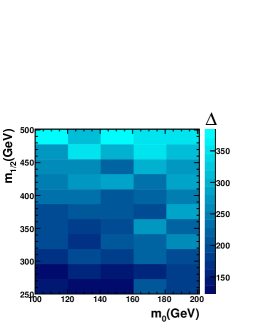
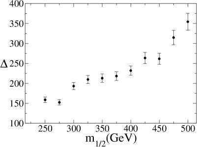
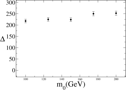
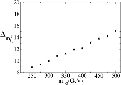
Fig. VIII shows that and have similar patterns of variation to and over , though the gradients are noticeably shallower. While we know and contribute to the Little Hierarchy Problem by giving a large contribution to , thereby requiring a cancellation to keep light, this shows there is also some tension in their own masses which restricts the parameter space. It is not clear from our results whether or not dimensionless variations are restricting different regions of parameter space to those in or if and are merely sub-volumes of , with no influence on . This topic deserves further study.
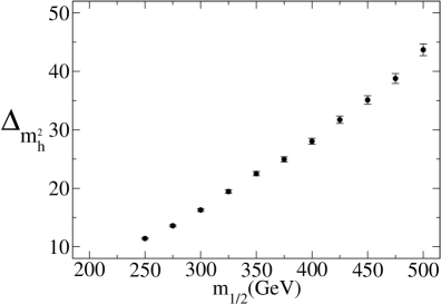
However our results do show some evidence that the Little Hierarchy Problem is not the only source of tuning. Displayed in Fig. IX is . Notice that is very small, so the errors are significantly reduced and we can resolve very small variations in . As with the other observables tuning increases with , but it is a distinctly non-linear variation. More surprising is that tuning decreases with . This pattern of variation, distinct from that shown for , shows a different source of tension. It can be understood by examining the one loop RGE solution for ,
| (39) |
where is a function of supersymmetry preserving parameters only, arising from the evolution of . Notice that there is some opportunity for a cancellation here to make lighter than expected. However the cancellation in the points we have looked at is very small, leading to small values for . As increases the already dominant positive part of the equation increases and increases. As this happens the cancellation becomes less significant to further reducing as shown in Fig. IX(bottom right). Increasing increases the size of the cancellation. If all other parameters on the right hand side of Eq. (39) were fixed then we would expect to see increase linearly444The effect of can be neglected since . with . However each point on our grid has the value of GeV fixed, and the term changes according to an inverted Eq. (38). This means is also increasing with and the balancing act between these two different effects leads to the nonlinear pattern shown.
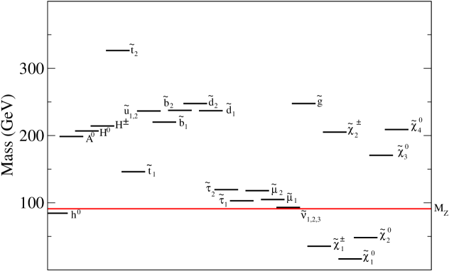
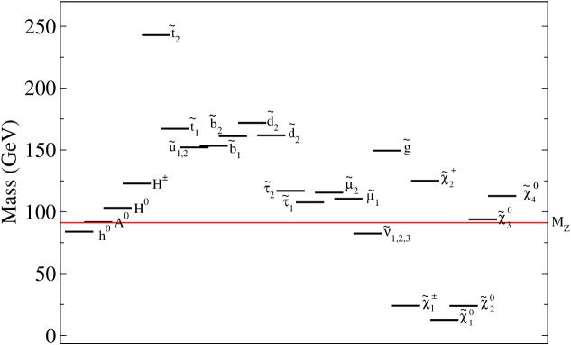
Although we can’t determine the normalisation using this approach it is nonetheless interesting to compare the unnormalised tunings for the points in our study with those obtained for points with more “natural” looking spectra. We present two points for this purpose. NP1 and NP2 are defined by,
| (40) |
The spectra of these points are displayed in Fig. X and Fig. XI, and the unnormalised tunings are displayed in Table 2. Note that these are not intended to be “realistic” scenarios. Indeed both NP1 and NP2 are ruled out by experiment but are simply intended to provide “natural” scenarios for comparison.
| NP1 | ||||||
|---|---|---|---|---|---|---|
| NP2 |
While NP1 has low values of , , and , it has a relatively large tuning in the mass of the lightest neutralino (). These combine to give a which is similar in size to the values found for our grid of points. In NP2 all of the tunings are relatively small, but the combined tuning is still larger than may naively have been anticipated. This is because many of these small tunings for individual observables are not correlated and are restricting different regions of parameter space. Table 3 shows the approximate relative magnitude of the tunings in our grid points with respect to these seemingly natural points.
| Relative to NP1 | ||||||
|---|---|---|---|---|---|---|
| Relative to NP2 |
In attempts to find a CMSSM scenario with a mass spectrum which is manifestly natural we found many scenarios where tuning appeared in the mass of the lightest neutralino. NP1 is a (moderate) example of this. This is because in some parameter choices, the lightest neutralino becomes very light due to large cancellations between the parameters. Other observables may also contain large cancellations between the parameters in certain regions of parameter space. While we have not studied this enough to make definitive claims, this may suggest that mass hierarchies appear in a greater proportion of the parameter space than conventional CMSSM wisdom dictates. This would reduce the true tuning in the CMSSM as scenarios with hierarchies would be less atypical than previously thought. A reduction in tuning from this effect can only be measured by using our normalised new measure, .
Unfortunately the numerical approach we have applied to the MSSM in this paper cannot be used to address this issue. An average measure of , over the whole parameter space, is needed in order to investigate this possibility. A thorough numerical survey of the parameter space would be too expensive, however an analytical study may be more promising. Findings in numerical studies like this may be used to identify which observables and parameters are important for fine tuning and therefore reduce the set and to a manageable size. We will not carry out this programme here, but leave it for a future study.
It is not just the possibility of finding a larger than expected global sensitivity which motivates this study. It may be that most of the CMSSM parameter space is hierarchy free and this is not a significant effect. However identifying a region of parameter space where mass hierarchies are common also opens up new possibilities. Past studies (see e.g. [51, 52]) have looked for a theoretical basis for relations between parameters which enforce a hierarchy between and . However no search has been made for theoretical relations which simply restrict the parameter space to regions where hierarchies, in general, are common. Such studies may also have the possibility of solving the Little Hierarchy Problem.
Here we have two complimentary approaches. An analytical approach which can determine tuning precisely, but is complicated and unwieldy when applied to a great number of parameters and observables and a numerical approach which can be applied to such situations but is not able to give an unambiguous measure of tuning as global sensitivity cannot be accounted for. Progress can be made by combing our two approaches. Since solving for the tuning analytically with all parameters and observables included would be difficult, one should first apply the numerical method. This might identify which observables are in tension and responsible for the restriction of parameter space and also along which axis in parameter space this restriction takes place. If these are a sufficiently small set (maybe no more than 5 parameters and 5 observables) then the analytical measure can be applied to this limited set to obtain a reasonably accurate and unambiguous measure of tuning for that model.
VII Conclusions
Fine tuning within the Standard Model has motivated many of the BSM theories which are popular within particle physics. In particular it motivates low energy supersymmetry. However constraints from LEP and other searches have placed stringent bounds on new physics which mean that many of the proposed solutions to the SM fine tuning problem also require tuning to some degree. In order to compare the viability of such models and judge whether or not they are satisfactory a reliable measure of tuning is required.
Current measures of tuning have several limitations. They neglect the many parameter nature of fine tuning, ignore additional tunings in other observables, consider local stability only and assume is parametrised in the same way as . In the literature there have been different approaches to combine tunings for individual parameters and observables. With no guiding principle to select one particular approach, which models are preferred in terms of naturalness can depend on which tuning measure is used.
In this paper we have presented a new measure of tuning based upon our intuitive notion of the restriction of parameter space. This measure can also be obtained by generalising the traditional measure of tuning to include many parameters, many observables and finite variations in the parameters followed by removing global sensitivity by factoring out the mean value of the unnormalised sensitivity.
From the application of this new measure to various toy models, we have shown that none of the other measures satisfactorily combine individual tunings per parameter. Interestingly though, in the absence of global sensitivity, it is the traditional measure of Barbieri and Guidice which comes closest to our result with deviations for these simple examples being very small.
A numerical approach for some CMSSM scenarios demonstrated how the tuning in complicated models with many parameters and many observables may be examined and also highlighted some of the complications and issues encountered in doing so.
Our new measure is needed in future studies to examine tuning in the boson mass and cosmological relic density simultaneously; to judge the true tuning in the NMSSM in light of [53]; to examine parametrisation choices which alleviate the tuning in different models and to study the global sensitivity of the complete tuning measure to see if this may cause a significant reduction in the tuning problem.
References
- [1] S. P. Martin, arXiv:hep-ph/9709356.
- [2] W. M. Yao et al. [Particle Data Group], J. Phys. G 33 (2006) 1.
- [3] S. Chang, P. J. Fox and N. Weiner, JHEP 0608, 068 (2006) [arXiv:hep-ph/0511250].
- [4] K. Choi, K. S. Jeong and K. i. Okumura, JHEP 0509 (2005) 039 [arXiv:hep-ph/0504037].
- [5] Y. Nomura and B. Tweedie, Phys. Rev. D 72, 015006 (2005) [arXiv:hep-ph/0504246].
- [6] K. Choi, K. S. Jeong, T. Kobayashi and K. i. Okumura, Phys. Lett. B 633 (2006) 355 [arXiv:hep-ph/0508029].
- [7] R. Kitano and Y. Nomura, Phys. Lett. B 631, 58 (2005) [arXiv:hep-ph/0509039].
- [8] O. Lebedev, H. P. Nilles and M. Ratz, arXiv:hep-ph/0511320.
- [9] R. Kitano and Y. Nomura, Phys. Rev. D 73, 095004 (2006) [arXiv:hep-ph/0602096].
- [10] S. Chang, L. J. Hall and N. Weiner, Phys. Rev. D 75, 035009 (2007) [arXiv:hep-ph/0604076].
- [11] J. A. Casas, J. R. Espinosa and I. Hidalgo, JHEP 0503, 038 (2005) [arXiv:hep-ph/0502066].
- [12] Z. Chacko, H. S. Goh and R. Harnik, Phys. Rev. Lett. 96, 231802 (2006) [arXiv:hep-ph/0506256].
- [13] Z. Chacko, H. S. Goh and R. Harnik, JHEP 0601, 108 (2006) [arXiv:hep-ph/0512088].
- [14] R. Barbieri and G. F. Giudice, Nucl. Phys. B 306, 63 (1988).
- [15] J. R. Ellis, K. Enqvist, D. V. Nanopoulos and F. Zwirner, Mod. Phys. Lett. A 1 (1986) 57.
- [16] B. de Carlos and J. A. Casas, Phys. Lett. B 309, 320 (1993) [arXiv:hep-ph/9303291].
- [17] B. de Carlos and J. A. Casas, arXiv:hep-ph/9310232.
- [18] P. H. Chankowski, J. R. Ellis and S. Pokorski, Phys. Lett. B 423, 327 (1998) [arXiv:hep-ph/9712234].
- [19] K. Agashe and M. Graesser, Nucl. Phys. B 507, 3 (1997) [arXiv:hep-ph/9704206].
- [20] D. Wright, arXiv:hep-ph/9801449.
- [21] G. L. Kane and S. F. King, Phys. Lett. B 451 (1999) 113 [arXiv:hep-ph/9810374].
- [22] M. Bastero-Gil, G. L. Kane and S. F. King, Phys. Lett. B 474, 103 (2000) [arXiv:hep-ph/9910506].
- [23] J. L. Feng, K. T. Matchev and T. Moroi, Phys. Rev. D 61, 075005 (2000) [arXiv:hep-ph/9909334].
- [24] B. C. Allanach, J. P. J. Hetherington, M. A. Parker and B. R. Webber, JHEP 0008, 017 (2000) [arXiv:hep-ph/0005186].
- [25] B. C. Allanach, Phys. Lett. B 635, 123 (2006) [arXiv:hep-ph/0601089].
- [26] T. Kobayashi, H. Terao and A. Tsuchiya, Phys. Rev. D 74, 015002 (2006) [arXiv:hep-ph/0604091].
- [27] R. Dermisek and J. F. Gunion, Phys. Rev. Lett. 95, 041801 (2005) [arXiv:hep-ph/0502105].
- [28] R. Barbieri and L. J. Hall, arXiv:hep-ph/0510243.
- [29] R. Barbieri, L. J. Hall and V. S. Rychkov, Phys. Rev. D 74, 015007 (2006) [arXiv:hep-ph/0603188].
- [30] B. Gripaios and S. M. West, Phys. Rev. D 74, 075002 (2006) [arXiv:hep-ph/0603229].
- [31] R. Dermisek, J. F. Gunion and B. McElrath, Phys. Rev. D 76 (2007) 051105 [arXiv:hep-ph/0612031].
- [32] G. W. Anderson and D. J. Castano, Phys. Lett. B 347, 300 (1995) [arXiv:hep-ph/9409419].
- [33] G. W. Anderson and D. J. Castano, Phys. Rev. D 52, 1693 (1995) [arXiv:hep-ph/9412322].
- [34] G. W. Anderson and D. J. Castano, Phys. Rev. D 53, 2403 (1996) [arXiv:hep-ph/9509212].
- [35] G. W. Anderson, D. J. Castano and A. Riotto, Phys. Rev. D 55, 2950 (1997) [arXiv:hep-ph/9609463].
- [36] J. A. Casas, J. R. Espinosa and I. Hidalgo, JHEP 0401, 008 (2004) [arXiv:hep-ph/0310137].
- [37] J. A. Casas, J. R. Espinosa and I. Hidalgo, arXiv:hep-ph/0402017.
- [38] J. A. Casas, J. R. Espinosa and I. Hidalgo, JHEP 0411, 057 (2004) [arXiv:hep-ph/0410298].
- [39] J. A. Casas, J. R. Espinosa and I. Hidalgo, Nucl. Phys. B 777 (2007) 226 [arXiv:hep-ph/0607279].
- [40] P. Ciafaloni and A. Strumia, Nucl. Phys. B 494, 41 (1997) [arXiv:hep-ph/9611204].
- [41] K. L. Chan, U. Chattopadhyay and P. Nath, Phys. Rev. D 58, 096004 (1998) [arXiv:hep-ph/9710473].
- [42] R. Barbieri and A. Strumia, Phys. Lett. B 433, 63 (1998) [arXiv:hep-ph/9801353].
- [43] L. Giusti, A. Romanino and A. Strumia, Nucl. Phys. B 550, 3 (1999) [arXiv:hep-ph/9811386].
- [44] P. H. Chankowski, J. R. Ellis, K. A. Olive and S. Pokorski, Phys. Lett. B 452, 28 (1999) [arXiv:hep-ph/9811284].
- [45] J. R. Ellis, K. A. Olive and Y. Santoso, New J. Phys. 4, 32 (2002) [arXiv:hep-ph/0202110].
- [46] S. F. King and J. P. Roberts, JHEP 0609 (2006) 036 [arXiv:hep-ph/0603095].
- [47] S. F. King and J. P. Roberts, JHEP 0701 (2007) 024 [arXiv:hep-ph/0608135].
- [48] B. C. Allanach, Comput. Phys. Commun. 143, 305 (2002) [arXiv:hep-ph/0104145].
- [49] V. D. Barger, M. S. Berger and P. Ohmann, Phys. Rev. D 49, 4908 (1994) [arXiv:hep-ph/9311269].
- [50] B. C. Allanach et al., Eur. Phys. J. C 25 (2002) 113 [arXiv:hep-ph/0202233].
- [51] P. H. Chankowski, J. R. Ellis, M. Olechowski and S. Pokorski, Nucl. Phys. B 544, 39 (1999) [arXiv:hep-ph/9808275].
- [52] G. L. Kane, J. D. Lykken, B. D. Nelson and L. T. Wang, Phys. Lett. B 551, 146 (2003) [arXiv:hep-ph/0207168].
- [53] P. C. Schuster and N. Toro, arXiv:hep-ph/0512189.