Non-Commutative Renormalization

Abstract

A new version of scale analysis and renormalization theory has been found on the non-commutative Moyal space. It could be useful for physics beyond the standard model or for standard physics in strong external field. The good news is that quantum field theory is better behaved on non-commutative than on ordinary space: indeed it has no Landau ghost. Noncommutativity might therefore be an alternative to supersymmetry. We review this rapidly growing subject.

1 Introduction

The world as we know it today is made of about 61 different scales if we use powers of ten. Indeed there is a fundamental length obtained by combining the three fundamental constants of physics, Newton’s gravitation constant $G$, Planck’s constant $\hbar$ and the speed of light $c$. It is the Planck length $\ell_{P}=\sqrt{\hbar G/c^{3}}$, whose value is about $1.6\;10^{-35}$ meters. Below this length ordinary space time almost certainly has to be quantized, so that the very notion of scale might be modified. But there is also a maximal observable scale or “horizon” in the universe, not for fundamental but for practical reasons. The current distance from the Earth to the edge of the visible universe is about 46 billion light-years in any direction. This translates into a comoving radius of the visible universe of about $4.4\;10^{26}$ meters, or more fundamentally $2.7\;10^{61}$ Planck lengths. Although we do not observe galaxies that far away, the WMAP data indicate that the universe is really at least 80% that big [1]. The geometric mean between the size of the (observable) universe and the Planck’s length stands therefore around $10^{-4}$ meters, about the size of an (arguably very small) ant. In [2], we proposed to call this the “antropic principle”.

Among the roughly sixty scales of the universe, only about ten to eleven were relatively well known to ancient Greeks and Romans two thousand years ago. We have now at least some knowledge of the 45 largest scales from $2\;10^{-19}$ meters (roughly speaking the scale of 1 Tev, observable at the largest particle colliders on earth) up to the size of the universe. This means that we know about three fourths of all scales. But the sixteen scales between $2\;10^{-19}$ meters and the Planck length form the last true terra incognita of physics. Note that this year the LHC accelerator at Cern with maximum energy of about 10 Tev should start opening a window into a new power of ten. But that truly special treat also will mark the end of an era. The next fifteen scales between $2.10^{-20}$ meters and the Planck length may remain largely out of direct reach in the foreseeable future, except for the glimpses which are expected to come from the study of very energetic but rare cosmic rays. Just as the Palomar mountain telescope remained the largest in the world for almost fifty years, we expect the LHC to remain the machine with highest energy for a rather long time until truly new technologies emerge. Therefore we should try to satisfy our understandable curiosity about the terra incognita in the coming decades through more and more sophisticated indirect analysis. Here theoretical and mathematical physics have a large part to play because they will help us to better compare and recoup many indirect observations, most of them probably coming from astrophysics and cosmology, and to make better educated guesses.

I would like now to argue both that quantum field theory and renormalization are some of the best tools at our disposal for such educated guesses, but also that very likely we shall also need some generalization of these concepts.

Quantum field theory or QFT provides a quantum description of particles and interactions which is compatible with special relativity [3]-[4]-[5]-[6]. It is certainly essential because it lies right at the frontier of the terra incognita. It is the accurate formalism at the shortest distances we know, between roughly the atomic scale of $10^{-10}$ meters, at which relativistic corrections to quantum mechanics start playing a significant role, up to the last known scale of a Tev or $2\;10^{-19}$ meters. Over the years it has evolved into the standard model which explains in great detail most experiments in particle physics and is contradicted by none. But it suffers from at least two flaws. First it is not yet compatible with general relativity, that is Einstein’s theory of gravitation. Second, the standard model incorporates so many different Fermionic matter fields coupled by Bosonic gauge fields that it seems more some kind of new Mendeleyev table than a fundamental theory. For these two reasons QFT and the standard model are not supposed to remain valid without any changes until the Planck length where gravitation should be quantized. They could in fact become inaccurate much before that scale.

What about renormalization? Nowadays renormalization is considered the heart of QFT, and even much more [7]-[8]-[9]. But initially renormalization was little more than a trick, a quick fix to remove the divergences that plagued the computations of quantum electrodynamics. These divergences were due to summations over exchanges of virtual particles with high momenta. Early renormalization theory succeeded in hiding these divergences into unobservable bare parameters of the theory. In this way the physical quantities, when expressed in terms of the renormalized parameters at observable scales, no longer showed any divergences. Mathematicians were especially scornful. But many physicists also were not fully satisfied. F. Dyson, one of the founding fathers of that early theory, once told me: “We believed renormalization would not last more than six months, just the time for us to invent something better…”

Surprisingly, renormalization survived and prospered. In the mid 50’s Landau and others found a key difficulty, called the Landau ghost or triviality problem, which plagued simple renormalizable QFT such as the $\phi^{4}_{4}$ theory or quantum electrodynamics. Roughly speaking Landau showed that the infinities supposedly taken out by renormalization were still there, because the bare coupling corresponding to a non zero renormalized coupling became infinite at a very small but finite scale. Although his argument was not mathematically fully rigorous, many physicists proclaimed QFT and renormalization dead and looked for a better theory. But in the early 70’s, against all odds, they both made a spectacular comeback. As a double consequence of better experiments but also of better computations, quantum electrodynamics was demoted of its possibly fundamental status and incorporated into the larger electroweak theory of Glashow, Weinberg and Salam. This electroweak theory is still a QFT but with a non-Abelian gauge symmetry. Motivated by this work ’t Hooft and Veltman proved that renormalization could be extended to non-Abelian gauge theories [10]. This difficult technical feat used the new technique of dimensional renormalization to better respect the gauge symmetry. The next and key step was the extraordinary discovery that such non-Abelian gauge theories no longer have any Landau ghost. This was done first by ’t Hooft in some unpublished work, then by D. Gross, H. D. Politzer and F. Wilczek [11]-[12]. D. Gross and F. Wilczek then used this discovery to convincingly formulate a non-Abelian gauge theory of strong interactions [13], the ones which govern nuclear forces, which they called quantum chromodynamics. Remark that in every key aspect of this striking recovery, renormalization was no longer some kind of trick. It took a life of its own.

But as spectacular as this story might be, something even more important happened to renormalization around that time. In the hands of K. Wilson [14] and others, renormalization theory went out of its QFT cradle. Its scope expanded considerably. Under the alas unfortunate name of renormalization group (RG), it was recognized as the right mathematical technique to move through the different scales of physics. More precisely over the years it became a completely general paradigm to study changes of scale, whether the relevant physical phenomena are classical or quantum, and whether they are deterministic or statistical. This encompasses in particular the full Boltzmann’s program to deduce thermodynamics from statistical mechanics and potentially much more. In the hands of Wilson, Kadanoff, Fisher and followers, RG allowed to much better understand phase transitions in statistical mechanics, in particular the universality of critical exponents [15]. The fundamental observation of K. Wilson was that the change from bare to renormalized actions is too complex a phenomenon to be described in a single step. Just like the trajectory of a complicated dynamical system, it must be studied step by step through a local evolution equation. To summarize, do not jump over many scales at once!

Let us make a comparison between renormalization and geometry. To describe a manifold, one needs a covering set of maps or atlas with crucial transition regions which must appear on different maps and which are glued through transition functions. One can then describe more complicated objects, such as bundles over a base manifold, through connections which allow to parallel transport objects in the fibers when one moves over the base.

Renormalization theory is both somewhat similar and somewhat different. It is some kind of geometry with a very sophisticated infinite dimensional“bundle” part which loosely speaking describes the effective actions. These actions flow in some infinite dimensional functional space. But at least until now the “base” part is quite trivial: it is a simple one-dimensional positive real axis, better viewed in fact as a full real axis if we use logarithmic scales. We have indeed both positive and negative scales around a reference scale of observation The negative or small spatial scales are called ultraviolet and the positive or large ones are called infrared in reference to the origin of the theory in electrodynamics. An elementary step from one scale to the next is called a renormalization group step. K. Wilson understood that there is an analogy between this step and the elementary evolution step of a dynamical system. This analogy allowed him to bring the techniques of classical dynamical systems into renormalization theory. One can say that he was able to see the classical structure hidden in QFT.

Working in the direction opposite to K. Wilson, G. Gallavotti and collaborators were able to see the quantum field theory structure hidden in classical dynamics. For instance they understood secular averages in celestial mechanics as a kind of renormalization [16]-[17]. In classical mechanics, small denominators play the role of high frequencies or ultraviolet divergences in ordinary RG. The interesting physics consists in studying the long time behavior of the classical trajectories, which is the analog of the infrared or large distance effects in statistical mechanics.

At first sight the classical structure discovered by Wilson in QFT and the quantum structure discovered by Gallavotti and collaborators in classical mechanics are both surprising because classical and QFT perturbation theories look very different. Classical perturbation theory, like the inductive solution of any deterministic equation, is indexed by trees, whether QFT perturbation theory is indexed by more complicated “Feynman graphs”, which contain the famous “loops” of anti-particles responsible for the ultraviolet divergences . But the classical trees hidden inside QFT were revealed in many steps, starting with Zimmermann (which called them forests…)[18] through Gallavotti and many others, until Kreimer and Connes viewed them as generators of Hopf algebras [19, 20, 21]. Roughly speaking the trees were hidden because they are not just subgraphs of the Feynman graphs. They picture abstract inclusion relations of the short distance connected components of the graph within the bigger components at larger scales. Gallavotti and collaborators understood why there is a structure on the trees which index the classical Poincaré-Lindstedt perturbation series similar to Zimmermann’s forests in quantum field perturbation theory.

Let us make an additional remark which points to another fundamental similarity between renormalization group flow and time evolution. Both seem naturally oriented flows. Microscopic laws are expected to determine macroscopic laws, not the converse. Time runs from past to future and entropy increases rather than decreases. This is philosophically at the heart of standard determinism. A key feature of Wilson’s RG is to have defined in a mathematically precise way which short scale information should be forgotten through coarse graining: it is the part corresponding to the irrelevant operators in the action. But coarse graining is also fundamental for the second law in statistical mechanics, which is the only law in classical physics which is “oriented in time” and also the one which can be only understood in terms of change of scales.

Whether this arrow common to RG and to time evolution is of a cosmological origin remains to be further investigated. We remark simply here that in the distant past the big bang has to be explored and understood on a logarithmic time scale. At the beginning of our universe important physics is the one at very short distance. As time passes and the universe evolves, physics at longer distances, lower temperatures and lower momenta becomes literally visible. Hence the history of the universe itself can be summarized as a giant unfolding of the renormalization group.

This unfolding can then be specialized into many different technical versions depending on the particular physical context, and the particular problem at hand. RG has the potential to provide microscopic explanations for many phenomenological theories. Hence it remains today a very active subject, with several important new brands developed in the two last decades at various levels of physical precision and of mathematical rigor. To name just a few of these brands:

- the RG around extended singularities governs the quantum behavior of condensed matter [23][24][25]. It should also govern the propagation of wave fronts and the long-distance scattering of particles in Minkowski space. Extended singularities alter dramatically the behavior of the renormalization group. For instance because the dimension of the extended singularity of the Fermi surface equals that of the space itself minus one, hence that of space-time minus two, local quartic Fermionic interactions in condensed matter in any dimension have the same power counting than two dimensional Fermionic field theories. This means that condensed matter in any dimension is similar to just renormalizable field theory. Among the main consequences, there is no critical mean field dimension in condensed matter except at infinity, but there is a rigorous way to handle non perturbative phase transitions such as the BCS formation of superconducting pairs through a dynamical $1/N$ expansion [26].

- the RG trajectories in dimension 2 between conformal theories with different central charges have been pioneered in [27]. Here the theory is less advanced, but again the $c$-theorem is a very tantalizing analog of Boltzmann’s H-theorem.

- the functional RG of [28] governs the behavior of many disordered systems. It might have wide applications from spin glasses to surfaces.

Let us return to our desire to glimpse into the terra incognita from currently known physics. We are in the uncomfortable situations of salmons returning to their birthplace, since we are trying to run against the RG flow. Many different bare actions lead to the same effective physics, so that we may be lost in a maze. However the region of terra incognita closest to us is still far from the Planck scale. In that region we can expect that any non renormalizable terms in the action generated at the Planck scale have been washed out by the RG flow and renormalizable theories should still dominate physics. Hence renormalizability remains a guiding principle to lead us into the maze of speculations at the entrance of terra incognita. Of course we should also be alert and ready to incorporate possible modifications of QFT as we progress towards the Planck scale, since we know that quantization of gravity at that scale will not happen through standard field theory.

String theory [29] is currently the leading candidate for such a quantum theory of gravitation. Tantalizingly the spectrum of massless particles of the closed string contains particles up to spin 2, hence contains a candidate for the graviton. Open strings only contain spin one massless particles such as gauge Bosons. Since closed strings must form out of open strings through interactions, it has been widely argued that string theory provides an explanation for the existence of quantum gravity as a necessary complement to gauge theories. This remains the biggest success of the theory up to now. It is also remarkable that string theory (more precisely membrane theory) allows some microscopic derivations of the Beckenstein-Hawking formula for blackhole entropy [30].

String theory also predicts two crucial features which are unobserved up to now, supersymmetry and six or seven new Kaluza-Klein dimensions of space time at short distance. Although no superpartner of any real particle has been found yet, there are some indirect indications of supersymmetry, such as the careful study of the flows of the running non-Abelian standard model gauge couplings. Extra dimensions might also be welcome, especially if they are significantly larger than the Planck scale, because they might provide an explanation for the puzzling weakness of gravitation with respect to other forces. Roughly speaking gravitation could be weak because in string theory it propagates very naturally into such extra dimensions in contrast with other interactions which may remain stuck to our ordinary four dimensional universe or “brane”.

But there are several difficulties with string theory which cast some doubt on its usefulness to guide us into the first scales of terra incognita. First the theory is really a very bold stroke to quantize gravity at the Planck scale, very far from current observations. This giant leap runs directly against the step by step philosophy of the RG. Second the mathematical structure of string theory is complicated up to the point where it may become depressing. For instance great effort is needed to put the string theory at two loops on some rigorous footing [31], and three loops seem almost hopeless. Third, there was for some time the hope that string theory and the phenomenology at lower energies derived from it might be unique. This hope has now vanished with the discovery of a very complicated landscape of different possible string vacua and associated long distance phenomenologies.

In view of these difficulties some physicists have started to openly criticize what they consider a disproportionate amount of intellectual resources devoted to the study of string theory compared to other alternatives [32].

I do not share these critics. I think in particular that string theory has been very successful as a brain storming tool. It has lead already to many spectacular insights into pure mathematics and geometry. But my personal bet would be that if somewhere in the mountains near the Planck scale string theory might be useful, or even correct, we should also search for other complementary and more reliable principles to guide us in the maze of waterways at the entrance of terra incognita. If these other complementary principles turn out to be compatible with string theory at higher scales, so much the better.

It is a rather natural remark that since gravity alters the very geometry of ordinary space, any quantum theory of gravity should quantize ordinary space, not just the phase space of mechanics, as quantum mechanics does. Hence at some point at or before the Planck scale we should expect the algebra of ordinary coordinates or observables to be generalized to a non commutative algebra. Alain Connes, Michel Dubois-Violette, Ali Chamseddine and others have forcefully advocated that the classical Lagrangian of the current standard model arises much more naturally on simple non-commutative geometries than on ordinary commutative Minkowsky space. We refer to Alain’s lecture here for these arguments. They remain in the line of Einstein’s classical unification of Maxwell’s electrodynamics equations through the introduction of a new four dimensional space-time. The next logical step seems to find the analog of quantum electrodynamics. It should be quantum field theory on non-commutative geometry, or NCQFT. The idea of NCQFT goes back at least to Snyders [33].

A second line of argument ends at the same conclusion. String theorists realized in the late 90’s that NCQFT is an effective theory of strings [34, 35]. Roughly this is because in addition to the symmetric tensor $g_{\mu\nu}$ the spectrum of the closed string also contains an antisymmetric tensor $B_{\mu\nu}$. There is no reason for this antisymmetric tensor not to freeze at some lower scale into a classical field, just as $g_{\mu\nu}$ is supposed to freeze into the classical metric of Einstein’s general relativity. But such a freeze of $B_{\mu\nu}$ precisely induces an effective non commutative geometry. In the simplest case of flat Riemannian metric and trivial constant antisymmetric tensor, the geometry is simply of the Moyal type; it reduces to a constant anticommutator between (Euclidean) space-time coordinates. This made NCQFT popular among string theorists. A good review of these ideas can be found in [36]

These two lines of arguments, starting at both ends of terra incognita converge to the same conclusion: there should be an intermediate regime between QFT and string theory where NCQFT is the right formalism. The breaking of locality and the appearance of cyclic-symmetric rather than fully symmetric interactions in NCQFT is fully consistent with this intermediate status of NCQFT between fields and strings. The ribbon graphs of NCQFT may be interpreted either as “thicker particle world-lines” or as “simplified open strings world-sheets” in which only the ends of strings appear but not yet their internal oscillations. However until recently a big stumbling block remained. The simplest NCQFT on Moyal space, such as $\phi^{\star 4}_{4}$, were found not to be renormalizable because of a surprising phenomenon called uv/ir mixing. Roughly speaking this $\phi^{\star 4}_{4}$ theory still has infinitely many ultraviolet divergent graphs but fewer than the ordinary $\phi^{4}_{4}$ theory. The new “ultraviolet convergent” graphs, such as the non-planar tadpole generate completely unexpected infrared divergences which are not of the renormalizable type [37].

However three years ago the solution out of this riddle was found. H. Grosse and R. Wulkenhaar in a brilliant series of papers discovered how to renormalize $\phi^{\star 4}_{4}$ [38, 39, 40]. This “revolution” happened quietly without mediatic fanfare, but it might turn out to develop into a good Ariane’s thread at the entrance of the maze. Indeed remember the argument of Wilson: renormalizable theories are the building blocks of physics because they are the ones who survive RG flows…

It is always very interesting to develop a new brand of RG, but that new brand on non commutative Moyal space is especially exciting. Indeed it changes the very definition of scales in a new and non trivial way. Therefore it may ultimately change our view of locality and causality, hence our very view of the deterministic relationship from small to large distances. It is fair to say that the same is true of string theory, where $T$-dualities also change small into large distances and vice-versa. But in contrast with string theory, this new brand of NCQFT is mathematically tractable, not at one or two loops, but as we shall see below, at any number of loops and probably even non-perturbatively! This just means that we can do complicated computations in these NCQFT’s with much more ease and confidence than in string theory.

The goal of these lectures is to present this new set of burgeoning ideas.

We start with a blitz introduction to standard renormalization group concepts in QFT: functional integration and Feynman graphs. The system of Feynman graphs of the $\phi^{4}_{4}$ theory provide the simplest example to play and experiment with the idea of renormalization. It is straightforward to analyze the basic scaling behavior of high energy subgraphs within graphs of lower energy. In this way one discovers relatively easily the most important physical effect under change of the observation scale, namely the flow of the coupling constant. It leads immediately to the fundamental difficulty associated to the short distance behavior of the theory, namely the Landau ghost or triviality problem. That ghost disappears in the “asymptotically free” non-Abelian gauge theories [11]-[12]. With hindsight this result might perhaps be viewed in a not so distant future as the first glimpse of NCQFT…

Grosse and Wulkenhaar realized that previous studies of NCQFT had used the wrong propagator! Moyal interactions were noticed to obey a certain Langmann-Szabo duality[41], which exchanges space and momentum variables. Grosse and Wulkenhaar realized that the propagator should be modified to also respect this symmetry [40]. This means that NCQFT on Moyal spaces has to be based on the Mehler kernel, which governs propagation in a harmonic potential, rather than on the heat kernel, which governs ordinary propagation in commutative space. Grosse and Wulkenhaar were able to compute for the first time the Mehler kernel in the matrix base which transforms the Moyal product into a matrix product. This is a real tour de force! The matrix based Mehler kernel is quasi-diagonal, and they were able to use their computation to prove perturbative renormalizability of the theory, up to some estimates which were finally proven in [42].

By matching correctly propagator and interaction to respect symmetries, Grosse and Wulkenhaar were following one of the main successful thread of quantum field theory. Their renormalizability result is in the direct footsteps of ’t Hooft and Veltman, who did the same for non Abelian gauge theories thirty years before. However I have often heard two main critics raised, which I would like to answer here.

The first critic is that it is no wonder that adding a harmonic potential gets rid of the infrared problem. It is naive because the harmonic potential is the only partner of the Laplacian under LS duality. No other infrared regulator would make the theory renormalizable. The theory has infinitely many degrees of freedom, and infinitely many divergent graphs, so the new BPHZ theorem obtained by Grosse and Wulkenhaar is completely non-trivial. In fact now that the RG flow corresponding to these theories is better understood, we understand the former uv/ir mixing just as an ordinary anomaly which signaled a missing marginal term in the Lagrangian under that RG flow.

The second and most serious critic is that since the Mehler kernel is not translation invariant, the Grosse and Wulkenhaar ideas will never be able to describe any mainstream physics in which there should be no preferred origin. This is just wrong but for a more subtle reason. We have shown that the Grosse-Wulkenhaar method can be extended to renormalize theories such as the Langmann-Szabo-Zarembo $\bar{\phi}\star\phi\star\bar{\phi}\star\phi$ model [43, 44, 45] in four dimensions or the Gross-Neveu model in two dimensions. In these theories the ordinary Mehler kernel is replaced by a related kernel which governs propagation of charged particles in a constant background field. This kernel, which we now propose to call the covariant Mehler kernel, is still not translation invariant because it depends on non translation-invariant gauge choice. It oscillates rather than decays when particles move away from a preferred origin. But in such theories physical observables, which are gauge invariant, do not feel that preferred origin. That’s why translation invariant phenomena can be described!

We proposed to call the whole new class of NCQFT theories built either on the Mehler kernel or on its covariant generalizations vulcanized (may be we should have spelled Wulkenized?) because renormalizability means that their structure resist under change of scale .

These newly discovered vulcanized theories or NCVQFT and their associated RG flows absolutely deserve a thorough and systematic investigation, not only because they may be relevant for physics beyond the standard model, but also (although this is often less emphasized) because they may provide explanation of non-trivial effective physics in our ordinary standard world whenever strong background gauge fields are present. Many examples come to mind, from various aspects of the quantum Hall effect to the behavior of two dimensional charged polymers under magnetic fields or even to quark confinement. In such cases appropriate generalizations of the vulcanized RG may be the right tool to show how the correct effective non-local interactions emerge out of local interactions.

At the Laboratoire de physique théorique at Orsay we have embarked on such a systematic investigation of NCVQFTs and of their RG flows. This program is also actively pursued elsewhere. Let us review briefly the main recent results and open problems.

• Multiscale Analysis

  The initial Grosse-Wulkenhaar breakthrough used sharp cutoffs in matrix space, which like sharp cutoffs in ordinary direct and momentum space are not so well suited to rigorous bounds and multiscale analysis. By replacing these cutoffs by smoother cutoffs which cut directly the Mehler parameter into slices, we could derive rigorously the estimates that were only numerically checked in [40] hence close the last gaps in the BPHZ theorem for vulcanized non commutative $\phi^{\star 4}_{4}$ [42]. We could also replace the somewhat cumbersome recursive use of the Polchinski equation [46] by more direct and explicit bounds in a multiscale analysis.

• Direct Space

  Although non translation invariant propagators and non local vertices are unfamiliar, the direct space representation of NCVQFT remains closer to our ordinary intuition than the matrix base. Using direct space methods, we have provided a new proof of the BPHZ theorem for vulcanized non commutative $\phi^{\star 4}_{4}$ [47]. We have also extended the Grosse-Wulkenhaar results to the $\bar{\phi}\star\phi\star\bar{\phi}\star\phi$ LSZ model [43]. Our proof relies on a multiscale analysis analogous to [42] but in direct space. It allows a more transparent understanding of the Moyality of the counterterms for planar subgraphs at higher scales when seen through external propagators at lower scales. This is the exact analog of the locality in ordinary QFT of general subgraphs at higher scales when seen through external propagators at lower scales. Such propagators do not distinguish short distance details, and ordinary locality could be summarized as the obvious remark that from far enough away any object looks roughly like a point. But Moyality could be summarized as a more surprising fact: viewed from lower RG scales, planar higher scale effects, which are the only ones large enough to require renormalization, look like Moyal products.

• Fermionic theories

  To enlarge the class of renormalizable non-commutative field theories and to attack the quantum Hall effect problem it is essential to extend the results of Grosse-Wulkenhaar to Fermionic theories. Vulcanized Fermionic propagators have been computed and their scaling properties established, both in matrix base and direct space, in [50]. They seem to be necessarily of the covariant type.

  The simplest Fermionic NCVQFT theory, corresponding to the two-dimensional ordinary Gross-Neveu model, was then proved renormalizable to all orders in [51]. This was done using the $x$-space version which seems also the most promising for a complete non-perturbative construction, using Pauli’s principle to control the apparent (fake) divergences of perturbation theory.

• Ghost Hunting

  Grosse and Wulkenhaar made the first non trivial one loop RG computation in NCVQFT in [52]. Although they did not word it initially in this way, their result means that at this order there is no Landau ghost in NCVQFT! A non trivial fixed point of the renormalization group develops at high energy, where the Grosse-Wulkenhaar parameter $\Omega$ tends to the self-dual point $\Omega=1$, so that Langmann-Szabo duality become exact, and the beta function vanishes. This stops the growth of the bare coupling constant in the ultraviolet regime, hence kills the ghost. So after all NCVQFT is not only as good as QFT with respect to renormalization, it is definitely better! This vindicates, although in a totally unexpected way, the initial intuition of Snyders [33], who like many after him was at least partly motivated by the hope to escape the divergences in QFT which were considered ugly. Remark however that the ghost is not killed because of asymptotic freedom. Both the bare and the renormalized coupling are non zero. They can be made both small if the renormalized $\Omega$ is not too small, in which case perturbation theory is expected to remain valid all along the complete RG trajectory. It is only in the singular limit $\Omega_{ren}\to 0$ that the ghost begins to reappear.

  For mathematical physicists who like me came from the constructive field theory program, the Landau ghost has always been a big frustration. Remember that because non Abelian gauge theories are very complicated and lead to confinement in the infrared regime, there is no good four dimensional rigorous field theory without unnatural cutoffs up to now. I was therefore from the start very excited by the possibility to build non perturbatively the $\phi^{\star 4}_{4}$ theory as the first such rigorous four dimensional field theory without unnatural cutoffs, even if it lives on the Moyal space which is not the one initially expected, and does not obey the usual axioms of ordinary QFT.

  For that happy scenario to happen, two main non trivial steps are needed. The first one is to extend the vanishing of the beta function at the self-dual point $\Omega=1$ to all orders of perturbation theory. This has been done in [57, 58], using the matrix version of the theory. First the result was checked by brute force computation at two and three loops. Then we devised a general method for all orders. It relies on Ward identities inspired by those of similar theories with quartic interactions in which the beta function vanishes [59, 60, 61]. However the relation of these Ward identities to the underlying LS symmetry remains unclear and we would also like to develop again an $x$-space version of that result to understand better its relation to the LS symmetry.

  The second step is to extend in a proper way constructive methods such as cluster and Mayer expansions to build non perturbatively the connected functions of NCVQFT in a single RG slice. Typically we would like a theorem of Borel summability [62] in the coupling constant for these functions which has to be uniform in the slice index. This is in progress. A construction of the model and of its full RG trajectory would then presumably follow from a multiscale analysis similar to that of [63].

• $\phi^{\star 3}_{6}$ and Kontsevich model

  The noncommutative $\phi^{\star 3}$ model in 6 dimensions has been shown to be renormalizable, asymptotically free, and solvable genus by genus by mapping it to the Kontsevich model, in [64, 65, 66]. The running coupling constant has also been computed exactly, and found to decrease more rapidly than predicted by the one-loop beta function. That model however is not expected to have a non-perturbative definition because it should be unstable at large $\phi$.

• Gauge theories

  A very important and difficult goal is to properly vulcanize gauge theories such as Yang-Mills in four dimensional Moyal space or Chern-Simons on the two dimensional Moyal plane plus one additional ordinary commutative time direction. We do not need to look at complicated gauge groups since the $U(1)$ pure gauge theory is non trivial and interacting on non commutative geometry even without matter fields. What is not obvious is to find a proper compromise between gauge and Langmann-Szabo symmetries which still has a well-defined perturbation theory around a computable vacuum after gauge invariance has been fixed through appropriate Faddeev-Popov or BRS procedures. We should judge success in my opinion by one main criterion, namely renormalizability. Recently de Goursac, Wallet and Wulkenhaar computed the non commutative action for gauge fields which can be induced through integration of a scalar renormalizable matter field minimally coupled to the gauge field [67]; the result exhibits both gauge symmetry and LS covariance, hence vulcanization, but the vacuum looks non trivial so that to check whether the associated perturbative expansion is really renormalizable seems difficult.

  Dimensional regularization and renormalization better respect gauge symmetries and they were the key to the initial ’tHooft-Veltman proof of renormalizability of ordinary gauge theories. Therefore no matter what the final word will be on NCV gauge theories, it should be useful to have the corresponding tools ready at hand in the non commutative context. This requires several steps, the first of which is

• Parametric Representation

  In this compact representation, direct space or momentum variables have been integrated out for each Feynman amplitude. The result is expressed as integrals over the heat kernel parameters of each propagator, and the integrands are the topological polynomials of the graph. These integrals can then be shown analytic in the dimension $D$ of space-time for $\Re D$ small enough. They are in fact meromorphic in the complex plane, and ultraviolet divergences can be extracted through appropriate inductive contour integrations.

  The same program can be accomplished in NCVQFT because the Mehler kernel is still quadratic in space variables. The corresponding topological hyperbolic polynomials are richer than in ordinary field theory since they are invariants of the ribbon graph which for instance contain information about the genus of the surface on which these graphs live. They can be computed both for ordinary NCVQFT [68] and in the more difficult case of covariant theories such as the LSZ model [69].

• Dimensional Regularization and Renormalization

  From the parametric representation the corresponding regularization and minimal dimensional renormalization scheme should follow for NCVQFTs. However appropriate factorization of the leading terms of the new hyperbolic polynomials under rescaling of the parameters of any subgraph is required. This is indeed the analog in the parameter representation of the “Moyality” of the counterterms in direct space. This program is under way [70].

• Quantum Hall Effect

  NCQFT and in particular the non commutative Chern Simons theory has been recognized as effective theory of the quantum hall effect already for some time [71]-[72]-[73]. We also refer to the lectures of V. Pasquier and of A. Polychronakos in this volume. But the discovery of the vulcanized RG holds promises for a better explanation of how these effective actions are generated from the microscopic level.

  In this case there is an interesting reversal of the initial Grosse-Wulkenhaar problematic. In the $\phi^{\star 4}_{4}$ theory the vertex is given a priori by the Moyal structure, and it is LS invariant. The challenge was to find the right propagator which makes the theory renormalizable, and it turned out to have LS duality.

  Now to explain the (fractional) quantum Hall effect, which is a bulk effect whose understanding requires electron interactions, we can almost invert this logic. The propagator is known since it corresponds to non-relativistic electrons in two dimensions in a constant magnetic field. It has LS duality. But the effective theory should be anionic hence not local. Here again we can argue that among all possible non-local interactions, a few renormalization group steps should select the only ones which form a renormalizable theory with the corresponding propagator. In the commutative case (i.e. zero magnetic field) local interactions such as those of the Hubbard model are just renormalizable in any dimension because of the extended nature of the Fermi-surface singularity. Since the non-commutative electron propagator (i.e. in non zero magnetic field) looks very similar to the Grosse-Wulkenhaar propagator (it is in fact a generalization of the Langmann-Szabo-Zarembo propagator) we can conjecture that the renormalizable interaction corresponding to this propagator should be given by a Moyal product. That’s why we hope that non-commutative field theory and a suitable generalization of the Grosse-Wulkenhaar RG might be the correct framework for a microscopic ab initio understanding of the fractional quantum Hall effect which is currently lacking.

• Charged Polymers in Magnetic Field

  Just like the heat kernel governs random motion, the covariant Mahler kernel governs random motion of charged particles in presence of a magnetic field. Ordinary polymers can be studied as random walk with a local self repelling or self avoiding interaction. They can be treated by QFT techniques using the $N=0$ component limit or the supersymmetry trick to erase the unwanted vacuum graphs. Many results, such as various exact critical exponents in two dimensions, approximate ones in three dimensions, and infrared asymptotic freedom in four dimensions have been computed for self-avoiding polymers through renormalization group techniques. In the same way we expect that charged polymers under magnetic field should be studied through the new non commutative vulcanized RG. The relevant interactions again should be of the Moyal rather than of the local type, and there is no reason that the replica trick could not be extended in this context. Ordinary observables such as $N$ point functions would be only translation covariant, but translation invariant physical observables such as density-density correlations should be recovered out of gauge invariant observables. In this way it might be possible to deduce new scaling properties of these systems and their exact critical exponents through the generalizations of the techniques used in the ordinary commutative case [74].

  More generally we hope that the conformal invariant two dimensional theories, the RG flows between them and the $c$ theorem of Zamolodchikov [27] should have appropriate magnetic generalizations which should involve vulcanized flows and Moyal interactions.

• Quark Confinement

  It is less clear that NCVQFT gauge theories might shed light on confinement, but this is also possible.

  Even for regular commutative field theory such as non-Abelian gauge theory, the strong coupling or non-perturbative regimes may be studied fruitfully through their non-commutative (i.e. non local) counterparts. This point of view is forcefully suggested in [35], where a mapping is proposed between ordinary and non-commutative gauge fields which do not preserve the gauge groups but preserve the gauge equivalent classes. Let us further remark that the effective physics of confinement should be governed by a non-local interaction, as is the case in effective strings or bags models. The great advantage of NCVQFT over the initial matrix model approach of ’tHooft [75] is that in the latter the planar graphs dominate because a gauge group $SU(N)$ with $N$ large is introduced in an ad hoc way instead of the physical $SU(2)$ or $SU(3)$, whether in the former case, there is potentially a perfectly physical explanation for the planar limit, since it should just emerge naturally out of a renormalization group effect. We would like the large $N$ matrix limit in NCVQFT’s to parallel the large $N$ vector limit which allows to understand the formation of Cooper pairs in supraconductivity [26]. In that case $N$ is not arbitrary but is roughly the number of effective quasi particles or sectors around the extended Fermi surface singularity at the superconducting transition temperature. This number is automatically very large if this temperature is very low. This is why we called this phenomenon a dynamical large $N$ vector limit. NCVQFTs provides us with the first clear example of a dynamical large $N$ matrix limit. We hope therefore that it should be ultimately useful to understand bound states in ordinary commutative non-Abelian gauge theories, hence quark confinement.

• Quantum Gravity

  Although ordinary renormalizable QFTs seem more or less to have NCVQFT analogs on the Moyal space, there is no renormalizable commutative field theory for spin 2 particles, so that the NCVQFTs alone should not allow quantization of gravity. However quantum gravity might enter the picture of NCVQFTs at a later and more advanced stage. Since quantum gravity appears in closed strings, it may have something to do with doubling the ribbons of some NCQFT in an appropriate way. But because there is no reason not to quantize the antisymmetric tensor $B$ which defines the non commutative geometry as well as the symmetric one $g$ which defines the metric, we should clearly no longer limit ourselves to Moyal spaces. A first step towards a non-commutative approach to quantum gravity along these lines should be to search for the proper analog of vulcanization in more general non-commutative geometries. It might for instance describe physics in the vicinity of a charged rotating black hole generating a strong magnetic field. However we have to admit that any theory of quantum gravity will probably remain highly conjectural for many decades or even centuries…

We would like to conclude this introduction on a slightly mind-provocative question: could non-commutativity be an attractive alternative to supersymmetry?

In the version of the standard model developped by Alain Connes and followers [76] there is some non commutative geometry but restricted to a very simple internal space. This model when fed with the spectral action principle reproduces in astonishing detail all the standard model terms. Furthermore it has some natural unification scale (without requiring a bigger non-Abelian gauge group and proton decay!). When prolonged through ordinary commutative renormalization group flows on ordinary $\mathbb{R}^{4}$ from that unification scale back to the Tev or Gev scales, it postdicts within a few percent the top quark mass and predicts the expected Higgs mass. Hence it seems a good starting point for understanding the standard model, just waiting for some additional fine tuning.

Now one of the strongest argument in favor of the existence of (still unobserved) supersymmetry is that it tames ultraviolet flows by adding loops of superpartners to the ordinary loops. In particular a main argument for supersymmetry is that it makes the three flows of the standard model $U(1)$, $SU(2)$ and $SU(3)$ couplings better converge at a single unification scale (see [77] and references therein for a discussion of this subtle question). The taming of loops by superpartners is also very important to improve the ultraviolet behavior of supergravity and ultimately of superstrings.

But we have now a new way to tame ultraviolet flows, namely non-commutativity of space-time! The mechanism which killed the Landau ghost could become therefore a substitute for supersymmetry, especially if superpartners are not found at the LHC.

If at some energy scale in the presumed “desert” (that is somewhere between the Tev and the Planck scale) non-commutativity escapes the internal space of A. Connes and invades ordinary space-time itself, it might manifest itself first in the form of a tiny non-zero commutator between pairs of space time variables. From that scale up towards grand unification and Planck scale, we should presumably use the non-commutative scale decomposition and the non-commutative renormalization group reviewed below rather than the ordinary one. Although we don’t know fully yet how non-Abelian gauge theories will behave in this respect, it may provide the neessary fine tuning of the Connes model. Just like for $\phi^{4}_{4}$, the flows should become milder and may grind to a halt.

In short the lack of Landau ghosts in non-commutative field theory discussed below means that non-commutative geometry might be an attractive alternative to supersymmetry to tame ultraviolet flows without introducing new particles.

Acknowledgments

I would like to warmly thank all the collaborators who contributed in various ways to the elaboration of this material, in particular M. Disertori, R. Gurau, J. Magnen, A. Tanasa, F. Vignes-Tourneret, J.C. Wallet and R. Wulkenhaar. Special thanks are due to F. Vignes-Tourneret since this review is largely based on our common recent review [78], with introduction and sections added on commutative renormalization, ghost hunting and the parametric representation. I would like also to sincerely apologize to the many people whose work in this area would be worth of citation but has not been cited here: this is because of my lack of time or competence but not out of bad will.

2 Commutative Renormalization, a Blitz Review

This section is a summary of [79] which we include for self-containedness.

2.1 Functional integral

In QFT, particle number is not conserved. Cross sections in scattering experiments contain the physical information of the theory. They are the matrix elements of the diffusion matrix ${\mathcal{S}}$. Under suitable conditions they are expressed in terms of the Green functions $G_{N}$ of the theory through so-called “reduction formulae”

Green’s functions are time ordered vacuum expectation values of the field $\phi$, which is operator valued and acts on the Fock space:

$$G_{N}(z_{1},...,z_{N})=<\psi_{0},T[\phi(z_{1})...\phi(z_{N})]\psi_{0}>\,.$$ (2.1)

Here $\psi_{0}$ is the vacuum state and the $T$-product orders $\phi(z_{1})...\phi(z_{N})$ according to times.

Consider a Lagrangian field theory, and split the total Lagrangian as the sum of a free plus an interacting piece, ${\mathcal{L}}={\mathcal{L}}_{0}+{\mathcal{L}}_{int}$. The Gell-Mann-Low formula expresses the Green functions as vacuum expectation values of a similar product of free fields with an $e^{i{\mathcal{L}}_{int}}$ insertion:

$$G_{N}(z_{1},...,z_{N})=\frac{<\psi_{0},T\biggl{[}\phi(z_{1})...\phi(z_{N})e^{i\int dx{\mathcal{L}}_{int}(\phi(x))}\biggr{]}\psi_{0}>}{<\psi_{0},T(e^{i\int dx{\mathcal{L}}_{int}(\phi(x))})\psi_{0}>}.$$ (2.2)

In the functional integral formalism proposed by Feynman [80], the Gell-Mann-Low formula is replaced by a functional integral in terms of an (ill-defined) “integral over histories” which is formally the product of Lebesgue measures over all space time. The corresponding formula is the Feynman-Kac formula:

$$G_{N}(z_{1},...,z_{N})==\frac{\int\prod\limits_{j}\phi(z_{j})e^{i\int{\mathcal{L}}(\phi(x))dx}D\phi}{\int e^{i\int{\mathcal{L}}(\phi(x))dx}D\phi}.$$ (2.3)

The integrand in (2.3) contains now the full Lagrangian ${\mathcal{L}}={\mathcal{L}}_{0}+{\mathcal{L}}_{int}$ instead of the interacting one. This is interesting to expose symmetries of the theory which may not be separate symmetries of the free and interacting Lagrangians, for instance gauge symmetries. Perturbation theory and the Feynman rules can still be derived as explained in the next subsection. But (2.3) is also well adapted to constrained quantization and to the study of non-perturbative effects. Finally there is a deep analogy between the Feynman-Kac formula and the formula which expresses correlation functions in classical statistical mechanics. For instance, the correlation functions for a lattice Ising model are given by

$$\bigl{<}\prod_{i=1}^{n}\sigma_{x_{i}}\bigr{>}=\frac{\sum\limits_{\{\sigma_{x}=\pm 1\}}e^{-L(\sigma)}\prod\limits_{i}\sigma_{x_{i}}}{\sum\limits_{\{\sigma_{x}=\pm 1\}}e^{-L(\sigma)}},$$ (2.4)

where $x$ labels the discrete sites of the lattice, the sum is over configurations $\{\sigma_{x}=\pm 1\}$ which associate a “spin” with value +1 or -1 to each such site and $L(\sigma)$ contains usually nearest neighbor interactions and possibly a magnetic field h:

$$L(\sigma)=\sum_{x,y\ {\rm nearest\ neighbors}}J\sigma_{x}\sigma_{y}+\sum_{x}h\sigma_{x}.$$ (2.5)

By analytically continuing (2.3) to imaginary time, or Euclidean space, it is possible to complete the analogy with (2.4), hence to establish a firm contact with statistical mechanics [15, 81, 82].

This idea also allows to give much better meaning to the path integral, at least for a free bosonic field. Indeed the free Euclidean measure can be defined easily as a Gaussian measure, because in Euclidean space $L_{0}$ is a quadratic form of positive type.

The Green functions continued to Euclidean points are called the Schwinger functions of the model, and are given by the Euclidean Feynman-Kac formula:

$$S_{N}(z_{1},...,z_{N})=Z^{-1}\int\prod_{j=1}^{N}\phi(z_{j})e^{-\int{\mathcal{L}}(\phi(x))dx}D\phi$$ (2.6)

$$Z=\int e^{-\int{\mathcal{L}}(\phi(x))dx}D\phi.$$ (2.7)

The simplest interacting field theory is the theory of a one component scalar bosonic field $\phi$ with quartic interaction $\lambda\phi^{4}$ ($\phi^{3}$ which is simpler is unstable). In ${\mathbb{R}}^{d}$ it is called the $\phi^{4}_{d}$ model. For $d=2,3$ the model is superrenormalizable and has been built non perturbatively by constructive field theory. For $d=4$ it is just renormalizable, and it provides the simplest pedagogical introduction to perturbative renormalization theory. But because of the Landau ghost Landau ghost or triviality problem explained in subsection 2.5, the model presumably does not exist as a true interacting theory at the non perturbative level. Its non commutative version should exist on the Moyal plane, see section 5.

Formally the Schwinger functions of $\phi^{4}_{d}$ are the moments of the measure:

$$d\nu=\frac{1}{Z}e^{-\frac{\lambda}{4!}\int\phi^{4}-(m^{2}/2)\int\phi^{2}-(a/2)\int(\partial_{\mu}\phi\partial^{\mu}\phi)}D\phi,$$ (2.8)

where

• $\lambda$ is the coupling constant, usually assumed positive or complex with positive real part; remark the convenient 1/4! factor to take into account the symmetry of permutation of all fields at a local vertex. In the non commutative version of the theory permutation symmetry becomes the more restricted cyclic symmetry and it is convenient to change the 1/4! factor to 1/4.

• $m$ is the mass, which fixes an energy scale for the theory;

• $a$ is the wave function constant. It can be set to 1 by a rescaling of the field.

• $Z$ is a normalization factor which makes (2.8) a probability measure;

• $D\phi$ is a formal (mathematically ill-defined) product $\prod\limits_{x\in{\mathbb{R}}^{d}}d\phi(x)$ of Lebesgue measures at every point of ${\mathbb{R}}^{d}$.

The Gaussian part of the measure is

$$d\mu(\phi)=\frac{1}{Z_{0}}e^{-(m^{2}/2)\int\phi^{2}-(a/2)\int(\partial_{\mu}\phi\partial^{\mu}\phi)}D\phi.$$ (2.9)

where $Z_{0}$ is again the normalization factor which makes (2.9) a probability measure.

More precisely if we consider the translation invariant propagator $C(x,y)\equiv C(x-y)$ (with slight abuse of notation), whose Fourier transform is

$$C(p)=\frac{1}{(2\pi)^{d}}\frac{1}{p^{2}+m^{2}},$$ (2.10)

we can use Minlos theorem and the general theory of Gaussian processes to define $d\mu(\phi)$ as the centered Gaussian measure on the Schwartz space of tempered distributions $S^{\prime}({\mathbb{R}}^{d})$ whose covariance is $C$. A Gaussian measure is uniquely defined by its moments, or the integral of polynomials of fields. Explicitly this integral is zero for a monomial of odd degree, and for $n=2p$ even it is equal to

$$\int\phi(x_{1})...\phi(x_{n})d\mu(\phi)=\sum_{\gamma}\prod_{\ell\in\gamma}C(x_{i_{\ell}},x_{j_{\ell}}),$$ (2.11)

where the sum runs over all the $2p!!=(2p-1)(2p-3)...5.3.1$ pairings $\gamma$ of the $2p$ arguments into $p$ disjoint pairs $\ell=(i_{\ell},j_{\ell})$.

Note that since for $d\geq 2$, $C(p)$ is not integrable, $C(x,y)$ must be understood as a distribution. It is therefore convenient to also use regularized kernels, for instance

$$C_{\kappa}(p)=\frac{1}{(2\pi)^{d}}\frac{e^{-\kappa(p^{2}+m^{2})}}{p^{2}+m^{2}}=\int_{\kappa}^{\infty}e^{-\alpha(p^{2}+m^{2})}d\alpha$$ (2.12)

whose Fourier transform $C_{\kappa}(x,y)$ is now a smooth function and not a distribution:

$$C_{\kappa}(x,y)=\int_{\kappa}^{\infty}e^{-\alpha m^{2}-(x-y)^{2}/4\alpha}\frac{d\alpha}{\alpha^{D/2}}$$ (2.13)

$\alpha^{-D/2}e^{-(x-y)^{2}/4\alpha}$ is the heat kernel and therefore this $\alpha$-representation has also an interpretation in terms of Brownian motion:

$$C_{\kappa}(x,y)=\int_{\kappa}^{\infty}d\alpha\exp(-m^{2}\alpha)\,P(x,y;\alpha)$$ (2.14)

where $P(x,y;\alpha)=(4\pi\alpha)^{-d/2}\exp(-{|x-y|}^{2}/4\alpha)$ is the Gaussian probability distribution of a Brownian path going from $x$ to $y$ in time $\alpha$.

Such a regulator $\kappa$ is called an ultraviolet cutoff, and we have (in the distribution sense) $\lim_{\kappa\to 0}C_{\kappa}(x,y)=C(x,y)$. Remark that due to the non zero $m^{2}$ mass term, the kernel $C_{\kappa}(x,y)$ decays exponentially at large $|x-y|$ with rate $m$. For some constant $K$ and $d>2$ we have:

$$|C_{\kappa}(x,y)|\leq K\kappa^{1-d/2}e^{-m|x-y|}.$$ (2.15)

It is a standard useful construction to build from the Schwinger functions the connected Schwinger functions, given by:

$$C_{N}(z_{1},...,z_{N})=\sum_{P_{1}\cup...\cup P_{k}=\{1,...,N\};\,P_{i}\cap P_{j}=0}(-1)^{k+1}(k-1)!\prod_{i=1}^{k}S_{p_{i}}(z_{j_{1}},...,z_{j_{p_{i}}}),$$ (2.16)

where the sum is performed over all distinct partitions of $\{1,...,N\}$ into $k$ subsets $P_{1},...,P_{k}$, $P_{i}$ being made of $p_{i}$ elements called $j_{1},...,j_{p_{i}}$. For instance in the $\phi^{4}$ theory, where all odd Schwinger functions vanish due to the unbroken $\phi\to-\phi$ symmetry, the connected 4-point function is simply:

$$C_{4}(z_{1},...,z_{4}) = S_{4}(z_{1},...,z_{4})-S_{2}(z_{1},z_{2})S_{2}(z_{3},z_{4})$$ (2.17)

$$\quad\quad-S_{2}(z_{1},z_{3})S_{2}(z_{2},z_{4})-S_{2}(z_{1},z_{4})S_{2}(z_{2},z_{3}).$$

2.2 Feynman Rules

The full interacting measure may now be defined as the multiplication of the Gaussian measure $d\mu(\phi)$ by the interaction factor:

$$d\nu=\frac{1}{Z}e^{-\frac{\lambda}{4!}\int\phi^{4}(x)dx}d\mu(\phi)$$ (2.18)

and the Schwinger functions are the normalized moments of this measure:

$$S_{N}(z_{1},...,z_{N})=\int\phi(z_{1})...\phi(z_{N})d\nu(\phi).$$ (2.19)

Expanding the exponential as a power series in the coupling constant $\lambda$, one obtains a formal expansion for the Schwinger functions:

$$S_{N}(z_{1},...,z_{N})=\frac{1}{Z}\sum_{n=0}^{\infty}\frac{(-\lambda)^{n}}{n!}\int\bigl{[}\int\frac{\phi^{4}(x)dx}{4!}\bigr{]}^{n}\phi(z_{1})...\phi(z_{N})d\mu(\phi)$$ (2.20)

It is now possible to perform explicitly the functional integral of the corresponding polynomial. The result gives at any order $n$ a sum over $(4n+N-1)!!$ “Wick contractions schemes ${\mathcal{W}}$”, i.e. ways of pairing together $4n+N$ fields into $2n+N/2$ pairs. At order $n$ the result of this perturbation scheme is therefore simply the sum over all these schemes ${\mathcal{W}}$ of the spatial integrals over $x_{1},...,x_{n}$ of the integrand $\prod_{\ell\in{\mathcal{W}}}C(x_{i_{\ell}},x_{j_{\ell}})$ times the factor $\frac{1}{n!}(\frac{-\lambda}{4!})^{n}$. These integrals are then functions (in fact distributions) of the external positions $z_{1},...,z_{N}$. But they may diverge either because they are integrals over all of ${\mathbb{R}}^{4}$ (no volume cutoff) or because of the singularities in the propagator $C$ at coinciding points.

Labeling the $n$ dummy integration variables in (2.20) as $x_{1},...,x_{n}$, we draw a line $\ell$ for each contraction of two fields. Each position $x_{1},...,x_{n}$ is then associated to a four-legged vertex and each external source $z_{i}$ to a one-legged vertex, as shown in Figure 1.

Figure 1: A possible contraction scheme with $n=N=4$.

For practical computations, it is obviously more convenient to gather all the contractions which lead to the same drawing, hence to the same integral. This leads to the notion of Feynman graphs. To any such graph is associated a contribution or amplitude, which is the sum of the contributions associated with the corresponding set of Wick contractions. The “Feynman rules” summarize how to compute this amplitude with its correct combinatoric factor.

We always use the following notations for a graph $G$:

• $n(G)$ or simply $n$ is the number of internal vertices of $G$, or the order of the graph.

• $l(G)$ or $l$ is the number of internal lines of $G$, i.e. lines hooked at both ends to an internal vertex of $G$.

• $N(G)$ or $N$ is the number of external vertices of $G$; it corresponds to the order of the Schwinger function one is looking at. When $N=0$ the graph is a vacuum graph, otherwise it is called an $N$-point graph.

• $c(G)$ or $c$ is the number of connected components of $G$,

• $L(G)$ or $L$ is the number of independent loops of G.

For a $regular$ $\phi^{4}$ graph, i.e. a graph which has no line hooked at both ends to external vertices, we have the relations:

$$l(G)=2n(G)-N(G)/2,$$ (2.21)

$$L(G)=l(G)-n(G)+c(G)=n(G)+1-N(G)/2.$$ (2.22)

where in the last equality we assume connectedness of $G$, hence $c(G)=1$.

A $subgraph$ $F$ of a graph $G$ is a subset of internal lines of $G$, together with the corresponding attached vertices. Lines in the subset defining $F$ are the internal lines of $F$, and their number is simply $l(F)$, as before. Similarly all the vertices of $G$ hooked to at least one of these internal lines of F are called the internal vertices of $F$ and considered to be in $F$; their number by definition is $n(F)$. Finally a good convention is to call external half-line of $F$ every half-line of $G$ which is not in $F$ but which is hooked to a vertex of $F$; it is then the number of such external half-lines which we call $N(F)$. With these conventions one has for $\phi^{4}$ subgraphs the same relation (2.21) as for regular $\phi^{4}$ graphs.

To compute the amplitude associated to a $\phi^{4}$ graph, we have to add the contributions of the corresponding contraction schemes. This is summarized by the “Feynman rules”:

• To each line $\ell$ with end vertices at positions $x_{\ell}$ and $y_{\ell}$, associate a propagator $C(x_{j},y_{j})$.

• To each internal vertex, associate $(-\lambda)/4!$.

• Count all the contraction schemes giving this diagram. The number should be of the form $(4!)^{n}n!/S(G)$ where $S(G)$ is an integer called the symmetry factor of the diagram. The $4!$ represents the permutation of the fields hooked to an internal vertex.

• Multiply all these factors, divide by $n!$ and sum over the position of all internal vertices.

The formula for the bare amplitude of a graph is therefore, as a distribution in $z_{1},....z_{N}$:

$$A_{G}(z_{1},...,z_{N})\equiv\int\prod_{i=1}^{n}dx_{i}\prod_{\ell\in G}C(x_{\ell},y_{\ell}).$$ (2.23)

This is the “direct” or “$x$-space” representation of a Feynman integral. As stated above, this integral suffers of possible divergences. But the corresponding quantities with both volume cutoff and ultraviolet cutoff $\kappa$ are well defined. They are:

$$A_{G,\Lambda}^{\kappa}(z_{1},...,z_{N})\equiv\int_{\Lambda^{n}}\prod_{i=1}^{n}dx_{i}\prod_{\ell\in G}C_{\kappa}(x_{\ell},y_{\ell}).$$ (2.24)

The integrand is indeed bounded and the integration domain is a compact box $\Lambda$.

The $unnormalized$ Schwinger functions are therefore formally given by the sum over all graphs with the right number of external lines of the corresponding Feynman amplitudes:

$$ZS_{N}=\sum_{\phi^{4}{\rm\ graphs\ }G{\rm\ with\ }N(G)=N}\frac{(-\lambda)^{n(G)}}{S(G)}A_{G}.$$ (2.25)

$Z$ itself, the normalization, is given by the sum of all vacuum amplitudes:

$$Z=\sum_{\phi^{4}{\rm\ graphs\ }G{\rm\ with\ }N(G)=0}\frac{(-\lambda)^{n(G)}}{S(G)}A_{G}.$$ (2.26)

Let us remark that since the total number of Feynman graphs is $(4n+N)!!$, taking into account Stirling’s formula and the symmetry factor $1/n!$ from the exponential we expect perturbation theory at large order to behave as $K^{n}n!$ for some constant $K$. Indeed at order $n$ the amplitude of a Feynman graph is a 4n-dimensional integral. It is reasonable to expect that in average it should behave as $c^{n}$ for some constant $c$. But this means that one should expect zero radius of convergence for the series (2.25). This is not too surprising. Even the one-dimensional integral

$$F(g)=\int_{-\infty}^{+\infty}e^{-x^{2}/2-\lambda x^{4}/4!}dx$$ (2.27)

is well-defined only for $\lambda\geq 0$. We cannot hope infinite dimensional functional integrals of the same kind to behave better than this one dimensional integral. In mathematically precise terms, $F$ is not analytic near $\lambda=0$, but only Borel summable [62]. Borel summability is therefore the best we can hope for the $\phi^{4}$ theory, and it has indeed been proved for the theory in dimensions 2 and 3 [83, 84].

From translation invariance, we do not expect $A_{G,\Lambda}^{\kappa}$ to have a limit as $\Lambda\to\infty$ if there are vacuum subgraphs in $G$. But we can remark that an amplitude factorizes as the product of the amplitudes of its connected components.

With simple combinatoric verification at the level of contraction schemes we can factorize the sum over all vacuum graphs in the expansion of unnormalized Schwinger functions, hence get for the normalized functions a formula analog to (2.25):

$$S_{N}=\sum_{\begin{subarray}{c}\scriptstyle\phi^{4}{\rm\ graphs\ }G{\rm\ with\ }N(G)=N\\ \scriptstyle G{\rm\ without\ any\ vacuum\ subgraph}\end{subarray}}\frac{(-\lambda)^{n(G)}}{S(G)}A_{G}.$$ (2.28)

Now in (2.28) it is possible to pass to the thermodynamic limit (in the sense of formal power series) because using the exponential decrease of the propagator, each individual graph has a limit at fixed external arguments. There is of course no need to divide by the volume for that because each connected component in (2.28) is tied to at least one external source, and they provide the necessary breaking of translation invariance.

Finally one can find the perturbative expansions for the connected Schwinger functions and the vertex functions. As expected, the connected Schwinger functions are given by sums over connected amplitudes:

$$C_{N}=\sum_{\phi^{4}{\rm\ connected\ graphs\ }G{\rm\ with\ }N(G)=N}\frac{(-\lambda)^{n(G)}}{S(G)}A_{G}$$ (2.29)

and the vertex functions are the sums of the $amputated$ amplitudes for proper graphs, also called one-particle-irreducible. They are the graphs which remain connected even after removal of any given internal line. The amputated amplitudes are defined in momentum space by omitting the Fourier transform of the propagators of the external lines. It is therefore convenient to write these amplitudes in the so-called momentum representation:

$$\Gamma_{N}(z_{1},...,z_{N})=\sum_{\phi^{4}{\rm\ proper\ graphs\ }G{\rm\ with\ }N(G)=N}\frac{(-\lambda)^{n(G)}}{S(G)}A_{G}^{T}(z_{1},...,z_{N}),$$ (2.30)

$$A_{G}^{T}(z_{1},...,z_{N})\equiv\frac{1}{(2\pi)^{dN/2}}\int dp_{1}...dp_{N}e^{i\sum p_{i}z_{i}}A_{G}(p_{1},...,p_{N}),$$ (2.31)

$$A_{G}(p_{1},...,p_{N})=\int\prod_{\ell\ {\rm internal\ line\ of\ }G}\frac{d^{d}p_{\ell}}{p_{\ell}^{2}+m^{2}}\prod_{v\in G}\delta(\sum_{\ell}\epsilon_{v,\ell}\;p_{\ell}).$$ (2.32)

Remark in (2.32) the $\delta$ functions which ensure momentum conservation at each internal vertex $v$; the sum inside is over both internal and external momenta; each internal line is oriented in an arbitrary way and each external line is oriented towards the inside of the graph. The incidence matrix $\epsilon(v,\ell)$ is 1 if the line $\ell$ arrives at $v$, -1 if it starts from $v$ and 0 otherwise. Remark also that there is an overall momentum conservation rule $\delta(p_{1}+...+p_{N})$ hidden in (2.32). The drawback of the momentum representation lies in the necessity for practical computations to eliminate the $\delta$ functions by a “momentum routing” prescription, and there is no canonical choice for that. Although this is rarely explicitly explained in the quantum field theory literature, such a choice of a momentum routing is equivalent to the choice of a particular spanning tree of the graph.

2.3 Scale Analysis and Renormalization

In order to analyze the ultraviolet or short distance limit according to the renormalization group method, we can cut the propagator $C$ into slices $C_{i}$ so that $C=\sum_{i=0}^{\infty}C_{i}$. This can be done conveniently within the parametric representation, since $\alpha$ in this representation roughly corresponds to $1/p^{2}$. So we can define the propagator within a slice as

$$C_{0}=\int_{1}^{\infty}e^{-m^{2}\alpha-\frac{|x-y|^{2}}{4\alpha}}\frac{d\alpha}{\alpha^{d/2}}\ ,\ \ C_{i}=\int_{M^{-2i}}^{M^{-2(i-1)}}e^{-m^{2}\alpha-\frac{|x-y|^{2}}{4\alpha}}\frac{d\alpha}{\alpha^{d/2}}\ \ {\rm for}\ i\geq 1.$$ (2.33)

where $M$ is a fixed number, for instance 10, or 2, or $e$ (see footnote 1 in the Introduction). We can intuitively imagine $C_{i}$ as the piece of the field oscillating with Fourier momenta essentially of size $M^{i}$. In fact it is easy to prove the bound (for $d>2$)

$$|C_{i}(x,y)|\leq K.M^{(d-2)i}e^{-M^{i}|x-y|}$$ (2.34)

where $K$ is some constant.

Now the full propagator with ultraviolet cutoff $M^{\rho}$, $\rho$ being a large integer, may be viewed as a sum of slices:

$$C_{\leq\rho}=\sum_{i=0}^{\rho}C_{i}$$ (2.35)

Then the basic renormalization group step is made of two main operations:

• A functional integration

• The computation of a logarithm

Indeed decomposing a covariance in a Gaussian process corresponds to a decomposition of the field into independent Gaussian random variables $\phi^{i}$, each distributed with a measure $d\mu_{i}$ of covariance $C_{i}$. Let us introduce

$$\Phi_{i}=\sum_{j=0}^{i}\phi_{j}.$$ (2.36)

This is the “low-momentum” field for all frequencies lower than $i$. The RG idea is that starting from scale $\rho$ and performing $\rho-i$ steps, one arrives at an effective action for the remaining field $\Phi_{i}$. Then, writing $\Phi_{i}=\phi_{i}+\Phi_{i-1}$, one splits the field into a “fluctuation” field $\phi_{i}$ and a “background” field $\Phi_{i-1}$. The first step, functional integration, is performed solely on the fluctuation field, so it computes

$$Z_{i-1}(\Phi_{i-1})=\int d\mu_{i}(\phi_{i})e^{-S_{i}(\phi_{i}+\Phi_{i-1})}.$$ (2.37)

Then the second step rewrites this quantity as the exponential of an effective action, hence simply computes

$$S_{i-1}(\Phi_{i-1})=-\log[Z_{i-1}(\Phi_{i-1})]$$ (2.38)

Now $Z_{i-1}=e^{-S_{i-1}}$ and one can iterate! The flow from the initial bare action $S=S_{\rho}$ for the full field to an effective renormalized action $S_{0}$ for the last “slowly varying” component $\phi_{0}$ of the field is similar to the flow of a dynamical system. Its evolution is decomposed into a sequence of discrete steps from $S_{i}$ to $S_{i-1}$.

This renormalization group strategy can be best understood on the system of Feynman graphs which represent the perturbative expansion of the theory. The first step, functional integration over fluctuation fields, means that we have to consider subgraphs with all their internal lines in higher slices than any of their external lines. The second step, taking the logarithm, means that we have to consider only connected such subgraphs. We call such connected subgraphs quasi-local. Renormalizability is then a non trivial result that combines locality and power counting for these quasi-local subgraphs.

Locality simply means that quasi-local subgraphs $S$ look local when seen through their external lines. Indeed since they are connected and since their internal lines have scale say $\geq i$, all the internal vertices are roughly at distance $M^{-i}$. But the external lines have scales $\leq i-1$, which only distinguish details larger than $M^{-(i-1)}$. Therefore they cannot distinguish the internal vertices of $S$ one from the other. Hence quasi-local subgraphs look like “fat dots” when seen through their external lines, see Figure 2. Obviously this locality principle is completely independent of dimension.

Figure 2: A high energy subgraph S seen from lower energies looks quasi-local.

Power counting is a rough estimate which compares the size of a fat dot such as $S$ in Figure 2 with $N$ external legs to the coupling constant that would be in front of an exactly local $\int\phi^{N}(x)dx$ interaction term if it were in the Lagrangian. To simplify we now assume that the internal scales are all equal to $i$, the external scales are $O(1)$, and we do not care about constants and so on, but only about the dependence in $i$ as $i$ gets large. We must first save one internal position such as the barycentre of the fat dot or the position of a particular internal vertex to represent the $\int dx$ integration in $\int\phi^{N}(x)dx$. Then we must integrate over the positions of all internal vertices of the subgraph save that one. This brings about a weight $M^{-di(n-1)}$, because since $S$ is connected we can use the decay of the internal lines to evaluate these $n-1$ integrals. Finally we should not forget the prefactor $M^{(D-2)li}$ coming from (2.34), for the $l$ internal lines. Multiplying these two factors and using relation (2.21)-(2.22) we obtain that the ”coupling constant” or factor in front of the fat dot is of order $M^{-di(n-1)+2i(2n-N/2)}=M^{\omega(G)}$, if we define the superficial degree of divergence of a $\phi^{4}_{d}$ connected graph as:

$$\omega(G)=(d-4)n(G)+d-\frac{d-2}{2}N(G).$$ (2.39)

So power counting, in contrast with locality, depends on the space-time dimension.

Let us return to the concrete example of Figure 2. A 4-point subgraph made of three vertices and four internal lines at a high slice $i$ index. If we suppose the four external dashed lines have much lower index, say of order unity, the subgraph looks almost local, like a fat dot at this unit scale. We have to save one vertex integration for the position of the fat dot. Hence the coupling constant of this fat dot is made of two vertex integrations and the four weights of the internal lines (in order not to forget these internal line factors we kept internal lines apparent as four tadpoles attached to the fat dot in the right of Figure 2). In dimension 4 this total weight turns out to be independent of the scale.

At lower scales propagators can branch either through the initial bare coupling or through any such fat dot in all possible ways because of the combinatorial rules of functional integration. Hence they feel effectively a new coupling which is the sum of the bare coupling plus all the fat dot corrections coming from higher scales. To compute these new couplings only graphs with $\omega(G)\geq 0$, which are called primitively divergent, really matter because their weight does not decrease as the gap $i$ increases.

- If $d=2$, we find $\omega(G)=2-2n$, so the only primitively divergent graphs have $n=1$, and $N=0$ or $N=2$. The only divergence is due to the “tadpole” loop $\int\frac{d^{2}p}{(p^{2}+m^{2})}$ which is logarithmically divergent.

- If $d=3$, we find $\omega(G)=3-n-N/2$, so the only primitively divergent graphs have $n\leq 3$, $N=0$, or $n\leq 2$ and $N=2$. Such a theory with only a finite number of “primitively divergent” subgraphs is called superrenormalizable.

- If $d=4$, $\omega(G)=4-N$. Every two point graph is quadratically divergent and every four point graph is logarithmically divergent. This is in agreement with the superficial degree of these graphs being respectively 2 and 0. The couplings that do not decay with $i$ all correspond to terms that were already present in the Lagrangian, namely $\int\phi^{4}$, $\int\phi^{2}$ and $\int(\nabla\phi).(\nabla\phi)$. Hence the structure of the Lagrangian resists under change of scale, although the values of the coefficients can change. The theory is called just renormalizable.

- Finally for $d>4$ we have infinitely many primitively divergent graphs with arbitrarily large number of external legs, and the theory is called non-renormalizable, because fat dots with $N$ larger than 4 are important and they correspond to new couplings generated by the renormalization group which are not present in the initial bare Lagrangian.

To summarize:

• Locality means that quasi-local subgraphs look local when seen through their external lines. It holds in any dimension.

• Power counting gives the rough size of the new couplings associated to these subgraphs as a function of their number $N$ of external legs, of their order $n$ and of the dimension of space time $d$.

• Renormalizability (in the ultraviolet regime) holds if the structure of the Lagrangian resists under change of scale, although the values of the coefficients or coupling constants may change. For $\phi^{4}$ it occurs if $d\leq 4$, with $d=4$ the most interesting case.

2.4 The BPHZ Theorem

The BPHZ theorem is both a brilliant historic piece of mathematical physics which gives precise mathematical meaning to the notion of renormalizability, using the mathematics of formal power series, but it is also ultimately a bad way to understand and express renormalization. Let us try to explain both statements.

For the massive Euclidean $\phi_{4}^{4}$ theory we could for instance state the following normalization conditions on the connected functions in momentum space at zero momenta:

$$C^{4}(0,0,0,0)=-\lambda_{ren},$$ (2.40)

$$C^{2}(p^{2}=0)=\frac{1}{m^{2}_{ren}},$$ (2.41)

$$\frac{d}{dp^{2}}C^{2}|_{p^{2}=0}=-\frac{a_{ren}}{m^{4}_{ren}}.$$ (2.42)

Usually one puts $a_{ren}=1$ by rescaling the field $\phi$.

Using the inversion theorem on formal power series for any fixed ultraviolet cutoff $\kappa$ it is possible to reexpress any formal power series in $\lambda_{bare}$ with bare propagators $1/(a_{bare}p^{2}+m^{2}_{bare})$ for any Schwinger functions as a formal power series in $\lambda_{ren}$ with renormalized propagators $1/(a_{ren}p^{2}+m^{2}_{ren})$. The BPHZ theorem then states that that formal perturbative formal power series has finite coefficients order by order when the ultraviolet cutoff $\kappa$ is lifted. The first proof by Hepp relied on the inductive Bogoliubov’s recursion scheme. Then a completely explicit expression for the coefficients of the renormalized series was written by Zimmermann and many followers. The coefficients of that renormalized series can be written as sums of renormalized Feynman amplitudes. They are similar to Feynman integrals but with additional subtractions indexed by Zimmermann’s forests. Returning to an inductive rather than explicit scheme, Polchinski remarked that it is possible to also deduce the BPHZ theorem from a renormalization group equation and inductive bounds which does not decompose each order of perturbation theory into Feynman graphs [46]. This method was clarified and applied by C. Kopper and coworkers, see [85].

The solution of the difficult “overlapping” divergence problem through Bogoliubov’s or Polchinski’s recursions and Zimmermann’s forests becomes particularly clear in the parametric representation using Hepp’s sectors. A Hepp sector is simply a complete ordering of the $\alpha$ parameters for all the lines of the graph. In each sector there is a different classification of forests into packets so that each packet gives a finite integral [86][87].

But from the physical point of view we cannot conceal the fact that purely perturbative renormalization theory is not very satisfying. At least two facts hint at a better theory which lies behind:

- The forest formula seems unnecessarily complicated, with too many terms. For instance in any given Hepp sector only one particular packet of forests is really necessary to make the renormalized amplitude finite, the one which corresponds to the quasi-local divergent subgraphs of that sector. The other packets seem useless, a little bit like “junk DNA”. They are there just because they are necessary for other sectors. This does not look optimal.

- The theory makes renormalized amplitudes finite, but at tremendous cost! The size of some of these renormalized amplitudes becomes unreasonably large as the size of the graph increases. This phenomenon is called the “renormalon problem”. For instance it is easy to check that the renormalized amplitude (at 0 external momenta) of the graphs $P_{n}$ with 6 external legs and $n+2$ internal vertices in Figure 3 becomes as large as $c^{n}n!$ when $n\to\infty$. Indeed at large $q$ the renormalized amplitude $A_{G_{2}}^{R}$ in Figure 5 grows like $\log|q|$. Therefore the chain of $n$ such graphs in Figure 3 behaves as $[\log|q|]^{n}$, and the total amplitude of $P_{n}$ behaves as

$$\int[\log|q|]^{n}\frac{d^{4}q}{[q^{2}+m^{2}]^{3}}\simeq_{n\to\infty}c^{n}n!$$ (2.43)

So after renormalization some families of graphs acquire so large values that they cannot be resumed! Physically this is just as bad as if infinities were still there.

Figure 3: A family of graphs $P_{n}$ producing a renormalon.

These two hints are in fact linked. As their name indicates, renormalons are due to renormalization. Families of completely convergent graphs such as the graphs $Q_{n}$ of Figure 4, are bounded by $c^{n}$, and produce no renormalons.

Figure 4: A family of convergent graphs $Q_{n}$, that do not produce any renormalon.

Studying more carefully renormalization in the $\alpha$ parametric representation one can check that renormalons are solely due to the forests packets that we compared to “junk DNA”. Renormalons are due to subtractions that are not necessary to ensure convergence, just like the strange $\log|q|$ growth of $A_{G_{0}}^{R}$ at large $q$ is solely due to the counterterm in the region where this counterterm is not necessary to make the amplitude finite.

We can therefore conclude that subtractions are not organized in an optimal way by the Bogoliubov recursion. What is wrong from a physical point of view in the BPHZ theorem is to use the size of the graph as the relevant parameter to organize Bogoliubov’s induction. It is rather the size of the line momenta that should be used to better organize the renormalization subtractions.

This leads to the point of view advocated in [9]: neither the bare nor the renormalized series are optimal. Perturbation should be organized as a power series in an infinite set of effective expansions, which are related through the RG flow equation. In the end exactly the same contributions are resumed than in the bare or in the renormalized series, but they are regrouped in a much better way.

2.5 The Landau ghost and Asymptotic Freedom

In the case of $\phi^{4}_{4}$ only the flow of the coupling constants really matters, because the flow of $m$ and of $a$ for different reasons are not very important in the ultraviolet limit:

- the flow of $m$ is governed at leading order by the tadpole. The bare mass $m^{2}_{i}$ corresponding to a finite positive physical mass $m^{2}_{ren}$ is negative and grows as $\lambda M^{2i}$ with the slice index $i$. But since $p^{2}$ in the $i$-th slice is also of order $M^{2i}$ but without the $\lambda$, as long as the coupling $\lambda$ remains small it remains much larger than $m^{2}_{i}$. Hence the mass term plays no significant role in the higher slices. It was remarked in [9] that because there are no overlapping problem associated to 1PI two point subgraphs, there is in fact no inconvenience to use the full renormalized $m_{ren}$ all the way from the bare to renormalized scales, with subtractions on 1PI two point subgraphs independent of their scale.

- the flow of $a$ is also not very important. Indeed it really starts at two loops because the tadpole is exactly local. So this flow is in fact bounded, and generates no renormalons. In fact as again remarked in [9] for theories of the $\phi^{4}_{4}$ type one might as well use the bare value $a_{bare}$ all the way from bare to renormalized scales and perform no second Taylor subtraction on any 1PI two point subgraphs,.

But the physics of $\phi^{4}_{4}$ in the ultraviolet limit really depends of the flow of $\lambda$. By a simple second order computation there are only 2 connected graphs with $n=2$ and $N=4$ pictured in Figure 5. They govern at leading order the flow of the coupling constant.

Figure 5: The $\phi^{4}$ connected graphs with $n=2$, $N=4$.

In the commutative $\phi^{4}_{4}$ theory the graph $G_{1}$ does not contribute to the coupling constant flow. This can be seen in many ways, for instance after mass renormalization the graph $G_{1}$ vanishes exactly because it contains a tadpole which is not quasi-local but exactly local. One can also remark that the graph is one particle reducible. In ordinary translation-invariant, hence momentum-conserving theories, one-particle-reducible quasi-local graphs never contribute significantly to RG flows. Indeed they become very small when the gap $i$ between internal and external scales grows. This is because by momentum conservation the momentum of any one-particle-reducible line $\ell$ has to be the sum of a finite set of external momenta on one of its sides. But a finite sum of small momenta remains small and this clashes directly with the fact that $\ell$ being internal its momentum should grow as the gap $i$ grows. Remark that this is no longer be true in non commutative vulcanized $\phi^{\star 4}_{4}$, because that theory is not translation invariant, and that’s why it will ultimately escape the Landau ghost curse.

So in $\phi^{4}_{4}$ the flow is intimately linked to the sign of the graph $G_{2}$ of Figure 5. More precisely, we find that at second order the relation between $\lambda_{i}$ and $\lambda_{i-1}$ is

$$\lambda_{i-1} \simeq \lambda_{i}-\beta\lambda_{i}^{2}$$ (2.44)

(remember the minus sign in the exponential of the action), where $\beta$ is a constant, namely the asymptotic value of $\sum_{j,j^{\prime}/\inf(j,j^{\prime})=i}\int d^{4}yC_{j}(x,y)C_{j^{\prime}}(x,y)$ when $i\to\infty$. Clearly this constant is positive. So for the normal stable $\phi_{4}^{4}$ theory, the relation (2.44) inverts into

$$\lambda_{i}\simeq\lambda_{i-1}+\beta\lambda_{i-1}^{2},$$ (2.45)

so that fixing the renormalized coupling seems to lead at finite $i$ to a large, diverging bare coupling, incompatible with perturbation theory. This is the Landau ghost problem, which affects both the $\phi^{4}_{4}$ theory and electrodynamics. Equivalently if one keeps $\lambda_{i}$ finite as $i$ gets large, $\lambda_{0}=\lambda_{ren}$ tends to zero and the final effective theory is “trivial” which means it is a free theory without interaction, in contradiction with the physical observation e.g. of a coupling constant of about $1/137$ in electrodynamics.

But in non-Abelian gauge theories an extra minus sign is created by the algebra of the Lie brackets. This surprising discovery has deep consequences. The flow relation becomes approximately

$$\lambda_{i}\simeq\lambda_{i-1}-\beta\lambda_{i}\lambda_{i-1},$$ (2.46)

with $\beta>0$, or, dividing by $\lambda_{i}\lambda_{i-1}$,

$$1/\lambda_{i}\simeq 1/\lambda_{i-1}+\beta,$$ (2.47)

with solution $\lambda_{i}\simeq\frac{\lambda_{0}}{1+\lambda_{0}\beta i}$. A more precise computation to third order in fact leads to

$$\lambda_{i}\simeq\frac{\lambda_{0}}{1+\lambda_{0}(\beta i+\gamma\log i+O(1))}.$$ (2.48)

Such a theory is called asymptotically free (in the ultraviolet limit) because the effective coupling tends to 0 with the cutoff for a finite fixed small renormalized coupling. Physically the interaction is turned off at small distances. This theory is in agreement with scattering experiments which see a collection of almost free particles (quarks and gluons) inside the hadrons at very high energy. This was the main initial argument to adopt quantum chromodynamics, a non-Abelian gauge theory with $SU(3)$ gauge group, as the theory of strong interactions [13].

Remark that in such asymptotically free theories which form the backbone of today’s standard model, the running coupling constants remain bounded between far ultraviolet “bare” scales and the lower energy scale where renormalized couplings are measured. Ironically the point of view on early renormalization theory as a trick to hide the ultraviolet divergences of QFT into infinite unobservable bare parameters could not turn out to be more wrong than in the standard model. Indeed the bare coupling constants tend to 0 with the ultraviolet cutoff, and what can be farther from infinity than 0?

3 Non-commutative field theory

3.1 Field theory on Moyal space

The recent progresses concerning the renormalization of non-commutative field theory have been obtained on a very simple non-commutative space namely the Moyal space. From the point of view of quantum field theory, it is certainly the most studied space. Let us start with its precise definition.

3.1.1 The Moyal space ${\mathbb{R}}^{D}_{\theta}$

Let us define $E=\left\{x^{\mu},\,\mu\in\llbracket 1,D\rrbracket\right\}$ and $\mathbb{C}\langle E\rangle$ the free algebra generated by $E$. Let $\Theta$ a $D\times D$ non-degenerate skew-symmetric matrix (which requires $D$ even) and $I$ the ideal of $\mathbb{C}\langle E\rangle$ generated by the elements $x^{\mu}x^{\nu}-x^{\nu}x^{\mu}-\imath\Theta^{\mu\nu}$. The Moyal algebra ${\mathcal{A}}_{\Theta}$ is the quotient $\mathbb{C}\langle E\rangle/I$. Each element in ${\mathcal{A}}_{\Theta}$ is a formal power series in the $x^{\mu}$’s for which the relation $\left[x^{\mu},x^{\nu}\right]=\imath\Theta^{\mu\nu}$ holds.

Usually, one puts the matrix $\Theta$ into its canonical form :

$$\Theta=\begin{pmatrix}\begin{matrix}0&\theta_{1}\\ -\theta_{1}&0\end{matrix}&&(0)\\ &\ddots&\\ (0)&&\begin{matrix}0&\theta_{D/2}\\ -\theta_{D/2}&0\end{matrix}\end{pmatrix}.$$ (3.1)

Sometimes one even set $\theta=\theta_{1}=\dotsm=\theta_{D/2}$. The preceeding algebraic definition whereas short and precise may be too abstract to perform real computations. One then needs a more analytical definition. A representation of the algebra ${\mathcal{A}}_{\Theta}$ is given by some set of functions on $\mathbb{R}^{d}$ equipped with a non-commutative product: the Groenwald-Moyal product. What follows is based on [88].

The Algebra ${\mathcal{A}}_{\Theta}$

The Moyal algebra ${\mathcal{A}}_{\Theta}$ is the linear space of smooth and rapidly decreasing functions ${\mathcal{S}}(\mathbb{R}^{D})$ equipped with the non-commutative product defined by: $\forall f,g\in{\mathcal{S}}_{D}\stackrel{{\scriptstyle\text{\tiny def}}}{{=}}{\mathcal{S}}(\mathbb{R}^{D})$,

$$(f\star_{\Theta}g)(x)= \int_{\mathbb{R}^{D}}\frac{d^{D}k}{(2\pi)^{D}}d^{D}y\,f(x+{\textstyle\frac{1}{2}}\Theta\cdot k)g(x+y)e^{\imath k\cdot y}$$ (3.2)

$$= \frac{1}{\pi^{D}\left|\det\Theta\right|}\int_{\mathbb{R}^{D}}d^{D}yd^{D}z\,f(x+y)g(x+z)e^{-2\imath y\Theta^{-1}z}\;.$$ (3.3)

This algebra may be considered as the “functions on the Moyal space $\mathbb{R}^{D}_{\theta}$”. In the following we will write $f\star g$ instead of $f\star_{\Theta}g$ and use : $\forall f,g\in{\mathcal{S}}_{D}$, $\forall j\in\llbracket 1,2N\rrbracket$,

$$({\mathscr{F}}f)(x)= \int f(t)e^{-\imath tx}dt$$ (3.4)

for the Fourier transform and

$$(f\diamond g)(x)= \int f(x-t)g(t)e^{2\imath x\Theta^{-1}t}dt$$ (3.5)

for the twisted convolution. As on $\mathbb{R}^{D}$, the Fourier transform exchange product and convolution:

$${\mathscr{F}}(f\star g)= {\mathscr{F}}(f)\diamond{\mathscr{F}}(g)$$ (3.6)

$${\mathscr{F}}(f\diamond g)= {\mathscr{F}}(f)\star{\mathscr{F}}(g).$$ (3.7)

One also shows that the Moyal product and the twisted convolution are associative:

$$((f\diamond g)\diamond h)(x)= \int f(x-t-s)g(s)h(t)e^{2\imath(x\Theta^{-1}t+(x-t)\Theta^{-1}s)}ds\,dt$$ (3.8)

$$= \int f(u-v)g(v-t)h(t)e^{2\imath(x\Theta^{-1}v-t\Theta^{-1}v)}dt\,dv$$

$$= (f\diamond(g\diamond h))(x).$$ (3.9)

Using (3.7), we show the associativity of the $\star$-product. The complex conjugation is involutive in ${\mathcal{A}}_{\Theta}$

$$\overline{f\star_{\Theta}g}= \bar{g}\star_{\Theta}\bar{f}.$$ (3.10)

One also have

$$f\star_{\Theta}g= g\star_{-\Theta}f.$$ (3.11)

Proposition 3.1 (Trace).

For all $f,g\in{\mathcal{S}}_{D}$,

$$\int dx\,(f\star g)(x)= \int dx\,f(x)g(x)=\int dx\,(g\star f)(x)\;.$$ (3.12)

Proof.

$$\int dx\,(f\star g)(x)= {\mathscr{F}}(f\star g)(0)=({\mathscr{F}}f\diamond{\mathscr{F}}g)(0)$$ (3.13)

$$= \int{\mathscr{F}}f(-t){\mathscr{F}}g(t)dt=({\mathscr{F}}f\ast{\mathscr{F}}g)(0)={\mathscr{F}}(fg)(0)$$

$$= \int f(x)g(x)dx$$

where $\ast$ is the ordinary convolution. ∎

In the following sections, we will need lemma 3.2 to compute the interaction terms for the $\Phi^{\star 4}_{4}$ and Gross-Neveu models. We write $x\wedge y\stackrel{{\scriptstyle\text{\tiny def}}}{{=}}2x\Theta^{-1}y$.

Lemma 3.2.

For all $j\in\llbracket 1,2n+1\rrbracket$, let $f_{j}\in{\mathcal{A}}_{\Theta}$. Then

$$\left(f_{1}\star_{\Theta}\dotsb\star_{\Theta}f_{2n}\right)(x)= \frac{1}{\pi^{2D}\det^{2}\Theta}\int\prod_{j=1}^{2n}dx_{j}f_{j}(x_{j})\,e^{-\imath x\wedge\sum_{i=1}^{2n}(-1)^{i+1}x_{i}}\,e^{-\imath\varphi_{2n}},$$ (3.14)

$$\left(f_{1}\star_{\Theta}\dotsb\star_{\Theta}f_{2n+1}\right)(x)= \frac{1}{\pi^{D}\det\Theta}\int\prod_{j=1}^{2n+1}dx_{j}f_{j}(x_{j})\,\delta\Big{(}x-\sum_{i=1}^{2n+1}(-1)^{i+1}x_{i}\Big{)}\,e^{-\imath\varphi_{2n+1}},$$ (3.15)

$$\forall p\in\mathbb{N},\,\varphi_{p}= \sum_{i<j=1}^{p}(-1)^{i+j+1}x_{i}\wedge x_{j}.$$ (3.16)

Corollary 3.3.

For all $j\in\llbracket 1,2n+1\rrbracket$, let $f_{j}\in{\mathcal{A}}_{\Theta}$. Then

$$\int dx\,\left(f_{1}\star_{\Theta}\dotsb\star_{\Theta}f_{2n}\right)(x)= \frac{1}{\pi^{D}\det\Theta}\int\prod_{j=1}^{2n}dx_{j}f_{j}(x_{j})\,\,\delta\Big{(}\sum_{i=1}^{2n}(-1)^{i+1}x_{i}\Big{)}e^{-\imath\varphi_{2n}},$$ (3.17)

$$\int dx\,\left(f_{1}\star_{\Theta}\dotsb\star_{\Theta}f_{2n+1}\right)(x)= \frac{1}{\pi^{D}\det\Theta}\int\prod_{j=1}^{2n+1}dx_{j}f_{j}(x_{j})\,e^{-\imath\varphi_{2n+1}},$$ (3.18)

$$\forall p\in\mathbb{N},\,\varphi_{p}= \sum_{i<j=1}^{p}(-1)^{i+j+1}x_{i}\wedge x_{j}.$$ (3.19)

The cyclicity of the product, inherited from proposition 3.1 implies: $\forall f,g,h\in{\mathcal{S}}_{D}$,

$$\langle f\star g,h\rangle= \langle f,g\star h\rangle=\langle g,h\star f\rangle$$ (3.20)

and allows to extend the Moyal algebra by duality into an algebra of tempered distributions.

Extension by Duality

Let us first consider the product of a tempered distribution with a Schwartz-class function. Let $T\in{\mathcal{S}}^{\prime}_{D}$ and $h\in{\mathcal{S}}_{D}$. We define $\langle T,h\rangle\stackrel{{\scriptstyle\text{\tiny def}}}{{=}}T(h)$ and $\langle T^{\ast},h\rangle=\overline{\langle T,\overline{h}\rangle}$.

Definition 3.1.

Let $T\in{\mathcal{S}}^{\prime}_{D}$, $f,h\in{\mathcal{S}}_{D}$, we define $T\star f$ and $f\star T$ by

$$\langle T\star f,h\rangle= \langle T,f\star h\rangle,$$ (3.21)

$$\langle f\star T,h\rangle= \langle T,h\star f\rangle.$$ (3.22)

For example, the identity ${\mathds{1}}$ as an element of ${\mathcal{S}}^{\prime}_{D}$ is the unity for the $\star$-product: $\forall f,h\in{\mathcal{S}}_{D}$,

$$\langle{\mathds{1}}\star f,h\rangle= \langle{\mathds{1}},f\star h\rangle$$ (3.23)

$$= \int(f\star h)(x)dx=\int f(x)h(x)dx$$

$$= \langle f,h\rangle.$$

We are now ready to define the linear space ${\mathcal{M}}$ as the intersection of two sub-spaces ${\mathcal{M}}_{L}$ and ${\mathcal{M}}_{R}$ of ${\mathcal{S}}^{\prime}_{D}$.

Definition 3.2 (Multipliers algebra).

$${\mathcal{M}}_{L}= \left\{S\in{\mathcal{S}}^{\prime}_{D}\mathrel{:}\forall f\in{\mathcal{S}}_{D},\,S\star f\in{\mathcal{S}}_{D}\right\},$$ (3.24)

$${\mathcal{M}}_{R}= \left\{R\in{\mathcal{S}}^{\prime}_{D}\mathrel{:}\forall f\in{\mathcal{S}}_{D},\,f\star R\in{\mathcal{S}}_{D}\right\},$$ (3.25)

$${\mathcal{M}}= {\mathcal{M}}_{L}\cap{\mathcal{M}}_{R}.$$ (3.26)

One can show that ${\mathcal{M}}$ is an associative $\ast$-algebra. It contains, among others, the identity, the polynomials, the $\delta$ distribution and its derivatives. Then the relation

$$\left[x^{\mu},x^{\nu}\right]= \imath\Theta^{\mu\nu},$$ (3.27)

often given as a definition of the Moyal space, holds in ${\mathcal{M}}$ (but not in ${\mathcal{A}}_{\Theta}$).

3.1.2 The $\Phi^{\star 4}$-theory on ${\mathbb{R}}^{4}_{\theta}$

The simplest non-commutative model one may consider is the $\Phi^{\star 4}$-theory on the four-dimensional Moyal space. Its Lagrangian is the usual (commutative) one where the pointwise product is replaced by the Moyal one:

$$S[\phi]= \int d^{4}x\Big{(}-\frac{1}{2}\partial_{\mu}\phi\star\partial^{\mu}\phi+\frac{1}{2}m^{2}\,\phi\star\phi+\frac{\lambda}{4}\phi\star\phi\star\phi\star\phi\Big{)}(x).$$ (3.28)

Thanks to the formula (3.3), this action can be explicitly computed. The interaction part is given by the corollary 3.3:

$$\int dx\,\phi^{\star 4}(x)= \int\prod_{i=1}^{4}dx_{i}\,\phi(x_{i})\,\delta(x_{1}-x_{2}+x_{3}-x_{4})e^{\imath\varphi},$$ (3.29)

$$\varphi= \sum_{i<j=1}^{4}(-1)^{i+j+1}x_{i}\wedge x_{j}.$$

The most obvious characteristic of the Moyal product is its non-locality. But its non-commutativity implies that the vertex of the model (3.28) is only invariant under cyclic permutation of the fields. This restricted invariance incites to represent the associated Feynman graphs with ribbon propagators. One can then make a clear distinction between planar and non-planar graphs. This will be detailed in section 4.

Thanks to the delta function in (3.29), the oscillation may be written in different ways:

$$\delta(x_{1}-x_{2}+x_{3}-x_{4})e^{\imath\varphi}= \delta(x_{1}-x_{2}+x_{3}-x_{4})e^{\imath x_{1}\wedge x_{2}+\imath x_{3}\wedge x_{4}}$$ (3.30a)

$$= \delta(x_{1}-x_{2}+x_{3}-x_{4})e^{\imath x_{4}\wedge x_{1}+\imath x_{2}\wedge x_{3}}$$ (3.30b)

$$= \delta(x_{1}-x_{2}+x_{3}-x_{4})\exp\imath(x_{1}-x_{2})\wedge(x_{2}-x_{3}).$$ (3.30c)

The interaction is real and positive:

$$\int\prod_{i=1}^{4}dx_{i}\phi(x_{i})\,\delta(x_{1}-x_{2}+x_{3}-x_{4})e^{\imath\varphi}$$ (3.31)

$$= \int dk\left(\int dxdy\,\phi(x)\phi(y)e^{\imath k(x-y)+\imath x\wedge y}\right)^{\!\!2}\in\mathbb{R}_{+}.$$

It is also translation invariant as shows equation (3.30c).

The property 3.1 implies that the propagator is the usual one: $\hat{C}(p)=1/(p^{2}+m^{2})$.

3.1.3 UV/IR mixing

In the article [89], Filk computed the Feynman rules corresponding to (3.28). He showed that the planar amplitudes equal the commutative ones whereas the non-planar ones give rise to oscillations coupling the internal and external legs. Hence contrary perhaps to overoptimistic initial expectations, non commutative geometry alone does not eliminate the ultraviolet divergences of QFT. Since there are infinitely many planar graphs with four external legs, the model (3.28) might at best be just renormalizable in the ultraviolet regime, as ordinary $\phi^{4}_{4}$.

In fact it is not. Minwalla, Van Raamsdonk and Seiberg discovered that the model (3.28) exhibits a new type of divergences making it non-renormalizable [37]. A typical example is the non-planar tadpole:

$$=\frac{\lambda}{12}\int\frac{d^{4}k}{(2\pi)^{4}}\frac{e^{ip_{\mu}k_{\nu}\Theta^{\mu\nu}}}{k^{2}+m^{2}}$$

$$=\frac{\lambda}{48\pi^{2}}\sqrt{\frac{m^{2}}{(\Theta p)^{2}}}K_{1}(\sqrt{m^{2}(\Theta p)^{2}})\operatorname*{\simeq}_{p\to 0}p^{-2}.$$ (3.32)

If $p\neq 0$, this amplitude is finite but, for small $p$, it diverges like $p^{-2}$. In other words, if we put an ultraviolet cut-off $\Lambda$ to the $k$-integral, the two limits $\Lambda\to\infty$ and $p\to 0$ do not commute. This is the UV/IR mixing phenomena. A chain of non-planar tadpoles, inserted in bigger graphs, makes divergent any function (with six points or more for example). But this divergence is not local and can’t be absorbed in a mass redefinition. This is what makes the model non-renormalizable. We will see in sections 6.4 and 7 that the UV/IR mixing results in a coupling of the different scales of the theory. We will also note that we should distinguish different types of mixing.

The UV/IR mixing was studied by several groups. First, Chepelev and Roiban [48] gave a power counting for different scalar models. They were able to identify the divergent graphs and to classify the divergences of the theories thanks to the topological data of the graphs. Then V. Gayral [90] showed that UV/IR mixing is present on all isospectral deformations (they consist in curved generalizations of the Moyal space and of the non-commutative torus). For this, he considered a scalar model (3.28) and discovered contributions to the effective action which diverge when the external momenta vanish. The UV/IR mixing is then a general characteristic of the non-commutative theories, at least on these deformations.

3.2 The Grosse-Wulkenhaar breakthrough

The situation remained unchanged until H. Grosse and R. Wulkenhaar discovered a way to define a renormalizable non-commutative model. We will detail their result in section 4 but the main message is the following. By adding an harmonic term to the Lagrangian (3.28),

$$S[\phi]= \int d^{4}x\Big{(}-\frac{1}{2}\partial_{\mu}\phi\star\partial^{\mu}\phi+\frac{\Omega^{2}}{2}(\tilde{x}_{\mu}\phi)\star(\tilde{x}^{\mu}\phi)+\frac{1}{2}m^{2}\,\phi\star\phi+\frac{\lambda}{4}\phi\star\phi\star\phi\star\phi\Big{)}(x)$$ (3.33)

where $\widetilde{x}=2\Theta^{-1}x$ and the metric is Euclidean, the model, in four dimensions, is renormalizable at all orders of perturbation [40]. We will see in section 7 that this additional term give rise to an infrared cut-off and allows to decouple the different scales of the theory. The new model (3.33), which we call vulcanized $\Phi^{\star 4}_{4}$, does not exhibit any mixing. This result is very important because it opens the way towards other non-commutative field theories. Remember that we call vulcanization the procedure consisting in adding a new term to a Lagrangian of a non-commutative theory in order to make it renormalizable, see footnote 9.

The propagator $C$ of this $\Phi^{4}$ theory is the kernel of the inverse operator $-\Delta+\Omega^{2}\widetilde{x}^{2}+m^{2}$. It is known as the Mehler kernel [91, 50]:

$$C(x,y)=\frac{\Omega^{2}}{\theta^{2}\pi^{2}}\int_{0}^{\infty}\frac{dt}{\sinh^{2}(2\widetilde{\Omega}t)}\,e^{-\frac{\widetilde{\Omega}}{2}\coth(2\widetilde{\Omega}t)(x-y)^{2}-\frac{\widetilde{\Omega}}{2}\tanh(2\widetilde{\Omega}t)(x+y)^{2}-m^{2}t}.$$ (3.34)

Langmann and Szabo remarked that the quartic interaction with Moyal product is invariant under a duality transformation. It is a symmetry between momentum and direct space. The interaction part of the model (3.33) is (see equation (3.17))

$$S_{\text{int}}[\phi]= \int d^{4}x\,\frac{\lambda}{4}(\phi\star\phi\star\phi\star\phi)(x)$$ (3.35)

$$= \int\prod_{a=1}^{4}d^{4}x_{a}\,\phi(x_{a})\,V(x_{1},x_{2},x_{3},x_{4})$$ (3.36)

$$= \int\prod_{a=1}^{4}\frac{d^{4}p_{a}}{(2\pi)^{4}}\,\hat{\phi}(p_{a})\,\hat{V}(p_{1},p_{2},p_{3},p_{4})$$ (3.37)

with

$$V(x_{1},x_{2},x_{3},x_{4})= \frac{\lambda}{4}\frac{1}{\pi^{4}\det\Theta}\delta(x_{1}-x_{2}+x_{3}-x_{4})\cos(2(\Theta^{-1})_{\mu\nu}(x_{1}^{\mu}x_{2}^{\nu}+x_{3}^{\mu}x_{4}^{\nu}))$$

$$\hat{V}(p_{1},p_{2},p_{3},p_{4})= \frac{\lambda}{4}(2\pi)^{4}\delta(p_{1}-p_{2}+p_{3}-p_{4})\cos(\frac{1}{2}\Theta^{\mu\nu}(p_{1,\mu}p_{2,\nu}+p_{3,\mu}p_{4,\nu}))$$

where we used a cyclic Fourier transform: $\hat{\phi}(p_{a})=\int dx\,e^{(-1)^{a}\imath p_{a}x_{a}}\phi(x_{a})$. The transformation

$$\hat{\phi}(p)\leftrightarrow\pi^{2}\sqrt{|\det\Theta|}\,\phi(x), \qquad p_{\mu}\leftrightarrow\widetilde{x}_{\mu}$$ (3.38)

exchanges (3.36) and (3.37). In addition, the free part of the model (3.28) isn’t covariant under this duality. The vulcanization adds a term to the Lagrangian which restores the symmetry. The theory (3.33) is then covariant under the Langmann-Szabo duality:

$$S[\phi;m,\lambda,\Omega]\mapsto \Omega^{2}\,S[\phi;\frac{m}{\Omega},\frac{\lambda}{\Omega^{2}},\frac{1}{\Omega}].$$ (3.39)

By symmetry, the parameter $\Omega$ is confined in $\left[0,1\right]$. Let us note that for $\Omega=1$, the model is invariant.

The interpretation of that harmonic term is not yet clear. But the vulcanization procedure already allowed to prove the renormalizability of several other models on Moyal spaces such that $\Phi^{\star 4}_{2}$ [39], $\phi^{3}_{2,4}$ [64, 65] and the LSZ models [43, 44, 45]. These last ones are of the type

$$S[\phi]= \int d^{n}x\Big{(}\frac{1}{2}\bar{\phi}\star(-\partial_{\mu}+\widetilde{x}_{\mu}+m)^{2}\phi+\frac{\lambda}{4}\bar{\phi}\star\phi\star\bar{\phi}\star\phi\Big{)}(x).$$ (3.40)

By comparison with (3.33), one notes that here the additional term is formally equivalent to a fixed magnetic background. Therefore such a model is invariant under magnetic translations which combine a translation and a phase shift on the field. This model is invariant under the above duality and is exactly soluble. Let us remark that the complex interaction in (3.40) makes the Langmann-Szabo duality more natural. It doesn’t need a cyclic Fourier transform. The $\phi^{\star 3}$ model at $\Omega=1$ also exhibits a soluble structure [64, 65, 66].

3.3 The non-commutative Gross-Neveu model

Apart from the $\Phi^{\star 4}_{4}$, the modified Bosonic LSZ model [47] and supersymmetric theories, we now know several renormalizable non-commutative field theories. Nevertheless they either are super-renormalizable ($\Phi^{\star 4}_{2}$ [39]) or (and) studied at a special point in the parameter space where they are solvable ($\Phi^{\star 3}_{2},\Phi^{\star 3}_{4}$ [64, 65], the LSZ models [43, 44, 45]). Although only logarithmically divergent for parity reasons, the non-commutative Gross-Neveu model is a just renormalizable quantum field theory as $\Phi^{\star 4}_{4}$. One of its main interesting features is that it can be interpreted as a non-local Fermionic field theory in a constant magnetic background. Then apart from strengthening the “vulcanization” procedure to get renormalizable non-commutative field theories, the Gross-Neveu model may also be useful for the study of the quantum Hall effect. It is also a good first candidate for a constructive study [9] of a non-commutative field theory as Fermionic models are usually easier to construct. Moreover its commutative counterpart being asymptotically free and exhibiting dynamical mass generation [92, 93, 94], a study of the physics of this model would be interesting.

The non-commutative Gross-Neveu model ($\text{GN}^{2}_{\Theta}$) is a Fermionic quartically interacting quantum field theory on the Moyal plane $\mathbb{R}^{2}_{\theta}$. The skew-symmetric matrix $\Theta$ is

$$\Theta= \begin{pmatrix}0&-\theta\\ \theta&0\end{pmatrix}.$$ (3.41)

The action is

$$S[\bar{\psi},\psi]= \int dx\left(\bar{\psi}\left(-\imath\not{\partial}+\Omega\not{\widetilde{x}}+m+\mu\,\gamma_{5}\right)\psi+V_{\text{o}}(\bar{\psi},\psi)+V_{\text{no}}(\bar{\psi},\psi)\right)(x)$$ (3.42)

where $\widetilde{x}=2\Theta^{-1}x$, $\gamma_{5}=\imath\gamma^{0}\gamma^{1}$ and $V=V_{\text{o}}+V_{\text{no}}$ is the interaction part given hereafter. The $\mu$-term appears at two-loop order. We use a Euclidean metric and the Feynman convention $\not{a}=\gamma^{\mu}a_{\mu}$. The $\gamma^{0}$ and $\gamma^{1}$ matrices form a two-dimensional representation of the Clifford algebra $\{\gamma^{\mu},\gamma^{\nu}\}=-2\delta^{\mu\nu}$. Let us remark that the $\gamma^{\mu}$’s are then skew- Hermitian: $\gamma^{\mu\dagger}=-\gamma^{\mu}$.

Propagator

The propagator corresponding to the action (3.42) is given by the following lemma:

Lemma 3.4 (Propagator [50]).

The propagator of the Gross-Neveu model is

$$C(x,y)= \int d\mu_{C}(\bar{\psi},\psi)\,\psi(x)\bar{\psi}(y)=\left(-\imath\not{\partial}+\Omega\not{\widetilde{x}}+m\right)^{-1}(x,y)$$ (3.43)

$$= \ \int_{0}^{\infty}dt\,C(t;x,y),$$

$$C(t;x,y)= \ -\frac{\Omega}{\theta\pi}\frac{e^{-tm^{2}}}{\sinh(2\widetilde{\Omega}t)}\,e^{-\frac{\widetilde{\Omega}}{2}\coth(2\widetilde{\Omega}t)(x-y)^{2}+\imath\Omega x\wedge y}$$ (3.44)

$$\times\left\{\imath\widetilde{\Omega}\coth(2\widetilde{\Omega}t)(\not{x}-\not{y})+\Omega(\not{\widetilde{x}}-\not{\widetilde{y}})-m\right\}e^{-2\imath\Omega t\gamma\Theta^{-1}\gamma}$$

with $\widetilde{\Omega}=\frac{2\Omega}{\theta}$ et $x\wedge y=2x\Theta^{-1}y$.
We also have $e^{-2\imath\Omega t\gamma\Theta^{-1}\gamma}=\cosh(2\widetilde{\Omega}t)\mathds{1}_{2}-\imath\frac{\theta}{2}\sinh(2\widetilde{\Omega}t)\gamma\Theta^{-1}\gamma$.

If we want to study a $N$-color model, we can consider a propagator diagonal in these color indices.

Interactions

Concerning the interaction part $V$, recall that (see corollary 3.3) for any $f_{1}$, $f_{2}$, $f_{3}$, $f_{4}$ in ${\mathcal{A}}_{\Theta}$,

$$\int dx\,\left(f_{1}\star f_{2}\star f_{3}\star f_{4}\right)(x)= \frac{1}{\pi^{2}\det\Theta}\int\prod_{j=1}^{4}dx_{j}f_{j}(x_{j})\,\delta(x_{1}-x_{2}+x_{3}-x_{4})e^{-\imath\varphi},$$ (3.45)

$$\varphi= \sum_{i<j=1}^{4}(-1)^{i+j+1}x_{i}\wedge x_{j}.$$ (3.46)

This product is non-local and only invariant under cyclic permutations of the fields. Then, contrary to the commutative Gross-Neveu model, for which there exits only one spinorial interaction, the $\text{GN}^{2}_{\Theta}$ model has, at least, six different interactions: the orientable ones

$$V_{\text{o}}=\phantom{+} \frac{\lambda_{1}}{4}\int dx\,\left(\bar{\psi}\star\psi\star\bar{\psi}\star\psi\right)(x)$$ (3.47a)

$$+ \frac{\lambda_{2}}{4}\int dx\,\left(\bar{\psi}\star\gamma^{\mu}\psi\star\bar{\psi}\star\gamma_{\mu}\psi\right)(x)$$ (3.47b)

$$+ \frac{\lambda_{3}}{4}\int dx\,\left(\bar{\psi}\star\gamma_{5}\psi\star\bar{\psi}\star\gamma_{5}\psi\right)(x),$$ (3.47c)

where $\psi$’s and $\bar{\psi}$’s alternate and the non-orientable ones

$$V_{\text{no}}=\phantom{+} \frac{\lambda_{4}}{4}\int dx\,\left(\psi\star\bar{\psi}\star\bar{\psi}\star\psi\right)(x)$$ (3.48a)

$$+ \frac{\lambda_{5}}{4}\int dx\,\left(\psi\star\gamma^{\mu}\bar{\psi}\star\bar{\psi}\star\gamma_{\mu}\psi\right)(x)$$ (3.48b)

$$+ \frac{\lambda_{6}}{4}\int dx\,\left(\psi\star\gamma_{5}\bar{\psi}\star\bar{\psi}\star\gamma_{5}\psi\right)(x).$$ (3.48c)

All these interactions have the same $x$ kernel thanks to the equation (3.45). The reason for which we call these interactions orientable or not will be clear in section 7.

4 Multi-scale analysis in the matrix basis

The matrix basis is a basis for Schwartz-class functions. In this basis, the Moyal product becomes a simple matrix product. Each field is then represented by an infinite matrix [88, 39, 95].

4.1 A dynamical matrix model

4.1.1 From the direct space to the matrix basis

In the matrix basis, the action (3.33) takes the form:

$$S[\phi]= (2\pi)^{D/2}\sqrt{\det\Theta}\Big{(}\frac{1}{2}\phi\Delta\phi+\frac{\lambda}{4}\operatorname*{Tr}\phi^{4}\Big{)}$$ (4.1)

where $\phi=\phi_{mn},\,m,n\in\mathbb{N}^{D/2}$ and

$$\Delta_{mn,kl}= \sum_{i=1}^{D/2}\Big{(}\mu_{0}^{2}+\frac{2}{\theta}(m_{i}+n_{i}+1)\Big{)}\delta_{ml}\delta_{nk}\ -\frac{2}{\theta}(1-\Omega^{2})$$ (4.2)

$$\Big{(}\sqrt{(m_{i}+1)(n_{i}+1)}\,\delta_{m_{i}+1,l_{i}}\delta_{n_{i}+1,k_{i}}+\sqrt{m_{i}n_{i}}\,\delta_{m_{i}-1,l_{i}}\delta_{n_{i}-1,k_{i}}\Big{)}\prod_{j\neq i}\delta_{m_{j}l_{j}}\delta_{n_{j}k_{j}}.$$

The (four-dimensional) matrix $\Delta$ represents the quadratic part of the Lagragian. The first difficulty to study the matrix model (4.1) is the computation of its propagator $G$ defined as the inverse of $\Delta$ :

$$\sum_{r,s\in\mathbb{N}^{D/2}}\Delta_{mn;rs}G_{sr;kl}=\sum_{r,s\in\mathbb{N}^{D/2}}G_{mn;rs}\Delta_{sr;kl}=\delta_{ml}\delta_{nk}.$$ (4.3)

Fortunately, the action is invariant under $SO(2)^{D/2}$ thanks to the form (3.1) of the $\Theta$ matrix. It implies a conservation law

$$\Delta_{mn,kl}= 0\iff m+k\neq n+l.$$ (4.4)

The result is [40, 39]

$$G_{m,m+h;l+h,l} =\frac{\theta}{8\Omega}\int_{0}^{1}d\alpha\,\dfrac{(1-\alpha)^{\frac{\mu_{0}^{2}\theta}{8\Omega}+(\frac{D}{4}-1)}}{(1+C\alpha)^{\frac{D}{2}}}\prod_{s=1}^{\frac{D}{2}}G^{(\alpha)}_{m^{s},m^{s}+h^{s};l^{s}+h^{s},l^{s}},$$ (4.5)

$$G^{(\alpha)}_{m,m+h;l+h,l} =\left(\frac{\sqrt{1-\alpha}}{1+C\alpha}\right)^{m+l+h}\sum_{u=\max(0,-h)}^{\min(m,l)}{\mathcal{A}}(m,l,h,u)\left(\frac{C\alpha(1+\Omega)}{\sqrt{1-\alpha}(1-\Omega)}\right)^{m+l-2u},$$

where ${\mathcal{A}}(m,l,h,u)=\sqrt{\binom{m}{m-u}\binom{m+h}{m-u}\binom{l}{l-u}\binom{l+h}{l-u}}$ and $C$ is a function in $\Omega$ : $C(\Omega)=\frac{(1-\Omega)^{2}}{4\Omega}$. The main advantage of the matrix basis is that it simplifies the interaction part: $\phi^{\star 4}$ becomes $\operatorname*{Tr}\phi^{4}$. But the propagator becomes very complicated.

Let us remark that the matrix model (4.1) is dynamical: its quadratic part is not trivial. Usually, matrix models are local.

Definition 4.1.

A matrix model is called local if $G_{mn;kl}=G(m,n)\delta_{ml}\delta_{nk}$ and non-local otherwise.

In the matrix theories, the Feynman graphs are ribbon graphs. The propagator $G_{mn;kl}$ is then represented by the Figure 6.

Figure 6: Matrix Propagator

In a local matrix model, the propagator preserves the index values along the trajectories (simple lines).

4.1.2 Topology of ribbon graphs

The power counting of a matrix model depends on the topological data of its graphs. The figure 7 gives two examples of ribbon graphs.

(a) Planar

(b) Non-planar

Figure 7: Ribbon Graphs

Each ribbon graph may be drawn on a two-dimensional manifold. Actually each graph defines a surface on which it is drawn. Let a graph $G$ with $V$ vertices, $I$ internal propagators (double lines) and $F$ faces (made of simple lines). The Euler characteristic

$$\chi= 2-2g=V-I+F$$ (4.6)

gives the genus $g$ of the manifold. One can make this clear by passing to the dual graph. The dual of a given graph $G$ is obtained by exchanging faces and vertices. The dual graphs of the $\Phi^{\star 4}$ theory are tesselations of the surfaces on which they are drawn. Moreover each direct face broken by external legs becomes, in the dual graph, a puncture. If among the $F$ faces of a graph, $B$ are broken, this graph may be drawn on a surface of genus $g=1-\frac{1}{2}(V-I+F)$ with $B$ punctures. The figure 8 gives the topological data of the graphs of the figure 7.

$\Longrightarrow$

$\left.\begin{array}[]{c}$V=3$\\ $I=3$\\ $F=2$\\ $B=2$\end{array}\right\}\Longrightarrow\ g=0$
$\Longrightarrow$           $\left.\begin{array}[]{c}$V=2$\\ $I=3$\\ $F=1$\\ $B=1$\end{array}\right\}\Longrightarrow\ g=1$

Figure 8: Topological Data of Ribbon Graphs

4.2 Multi-scale analysis

In [42], a multi-scale analysis was introduced to complete the rigorous study of the power counting of the non-commutative $\Phi^{\star 4}$ theory.

4.2.1 Bounds on the propagator

Let $G$ a ribbon graph of the $\Phi^{\star 4}_{4}$ theory with $N$ external legs, $V$ vertices, $I$ internal lines and $F$ faces. Its genus is then $g=1-\frac{1}{2}(V-I+F)$. Four indices $\{m,n;k,l\}\in\mathbb{N}^{2}$ are associated to each internal line of the graph and two indices to each external line, that is to say $4I+2N=8V$ indices. But, at each vertex, the left index of a ribbon equals the right one of the neighbor ribbon. This gives rise to $4V$ independent identifications which allows to write each index in terms of a set $\mathcal{I}$ made of $4V$ indices, four per vertex, for example the left index of each half-ribbon.

The graph amplitude is then

$$A_{G}=\sum_{\mathcal{I}}\prod_{\delta\in G}G_{m_{\delta}(\mathcal{I}),n_{\delta}(\mathcal{I});k_{\delta}(\mathcal{I}),l_{\delta}(\mathcal{I})}\;\delta_{m_{\delta}-l_{\delta},n_{\delta}-k_{\delta}}\;,$$ (4.7)

where the four indices of the propagator $G$ of the line $\delta$ are function of $\mathcal{I}$ and written
$\{m_{\delta}(\mathcal{I}),n_{\delta}(\mathcal{I});k_{\delta}(\mathcal{I}),l_{\delta}(\mathcal{I})\}$. We decompose each propagator, given by (4.5):

$$G=\sum_{i=0}^{\infty}G^{i}\qquad\text{thanks to }\int_{0}^{1}d\alpha=\sum_{i=1}^{\infty}\int_{M^{-2i}}^{M^{-2(i-1)}}d\alpha,\;M>1.$$ (4.8)

We have an associated decomposition for each amplitude

$$A_{G} =\sum_{\mu}A_{G,\mu}\;,$$ (4.9)

$$A_{G,\mu} =\sum_{\mathcal{I}}\prod_{\delta\in G}G^{i_{\delta}}_{m_{\delta}(\mathcal{I}),n_{\delta}(\mathcal{I});k_{\delta}(\mathcal{I}),l_{\delta}(\mathcal{I})}\;\delta_{m_{\delta}(\mathcal{I})-l_{\delta}(\mathcal{I}),n_{\delta}(\mathcal{I})-k_{\delta}(\mathcal{I})}\;,$$ (4.10)

where $\mu=\{i_{\delta}\}$ runs over the all possible assignments of a positive integer $i_{\delta}$ to each line $\delta$. We proved the following four propositions:

Proposition 4.1.

For $M$ large enough, there exists a constant $K$ such that, for $\Omega\in[0.5,1]$, we have the uniform bound

$$G^{i}_{m,m+h;l+h,l}\leqslant KM^{-2i}e^{-\frac{\Omega}{3}M^{-2i}\|m+l+h\|}.$$ (4.11)

Proposition 4.2.

For $M$ large enough, there exists two constants $K$ and $K_{1}$ such that, for $\Omega\in[0.5,1]$, we have the uniform bound

$$G^{i}_{m,m+h;l+h,l}$$

$$\leqslant KM^{-2i}e^{-\frac{\Omega}{4}M^{-2i}\|m+l+h\|}\prod_{s=1}^{\frac{D}{2}}\min\left(1,\left(\frac{K_{1}\min(m^{s},l^{s},m^{s}+h^{s},l^{s}+h^{s})}{M^{2i}}\right)^{\!\!\frac{|m^{s}-l^{s}|}{2}}\right).$$ (4.12)

This bound allows to prove that the only diverging graphs have either a constant index along the trajectories or a total jump of $2$.

Proposition 4.3.

For $M$ large enough, there exists a constant $K$ such that, for $\Omega\in[\frac{2}{3},1]$, we have the uniform bound

$$\sum_{l=-m}^{p}G^{i}_{m,p-l,p,m+l} \leqslant KM^{-2i}\,e^{-\frac{\Omega}{4}M^{-2i}(\|p\|+\|m\|)}\;.$$ (4.13)

This bound shows that the propagator is almost local in the following sense: with $m$ fixed, the sum over $l$ doesn’t cost anything (see Figure 6). Nevertheless the sums we’ll have to perform are entangled (a given index may enter different propagators) so that we need the following proposition.

Proposition 4.4.

For $M$ large enough, there exists a constant $K$ such that, for $\Omega\in[\frac{2}{3},1]$, we have the uniform bound

$$\sum_{l=-m}^{\infty}\max_{p\geqslant\max(l,0)}G^{i}_{m,p-l;p,m+l}\leqslant KM^{-2i}e^{-\frac{\Omega}{36}M^{-2i}\|m\|}\;.$$ (4.14)

We refer to [42] for the proofs of these four propositions.

4.2.2 Power counting

About half of the $4V$ indices initially associated to a graph is determined by the external indices and the delta functions in (4.7). The other indices are summation indices. The power counting consists in finding which sums cost $M^{2i}$ and which cost $\mathcal{O}(1)$ thanks to (4.13). The $M^{2i}$ factor comes from (4.11) after a summation over an index $m\in\mathbb{N}^{2}$,

$$\sum_{m^{1},m^{2}=0}^{\infty}e^{-cM^{-2i}(m^{1}+m^{2})}=\frac{1}{(1-e^{-cM^{-2i}})^{2}}=\frac{M^{4i}}{c^{2}}(1+\mathcal{O}(M^{-2i})).$$ (4.15)

We first use the delta functions as much as possible to reduce the set $\mathcal{I}$ to a true minimal set ${\mathcal{I}}^{\prime}$ of independent indices. For this, it is convenient to use the dual graphs where the resolution of the delta functions is equivalent to a usual momentum routing.

The dual graph is made of the same propagators than the direct graph except the position of their indices. Whereas in the original graph we have $G_{mn;kl}=\raisebox{-4.30554pt}{\includegraphics[scale={.6}]{oberfig-16.pdf}}$, the position of the indices in a dual propagator is

$$G_{mn;kl}=\raisebox{-4.30554pt}{\includegraphics[scale={.6}]{oberfig-17.pdf}}\;.$$ (4.16)

The conservation $\delta_{l-m,-(n-k)}$ in (4.7) implies that the difference $l-m$ is conserved along the propagator. These differences behave like angular momenta and the conservation of the differences $\ell=l-m$ and $-\ell=n-k$ is nothing else than the conservation of the angular momentum thanks to the symmetry $SO(2)\times SO(2)$ of the action (4.1):

$$\qquad l=m+\ell\;,\leavevmode\nobreak\ \leavevmode\nobreak\ n=k+(-\ell).$$ (4.17)

The cyclicity of the vertices implies the vanishing of the sum of the angular momenta entering a vertex. Thus the angular momentum in the dual graph behaves exactly like the usual momentum in ordinary Feynman graphs.

We know that the number of independent momenta is exactly the number $L^{\prime}$ ($=I-V^{\prime}+1$ for a connected graph) of loops in the dual graph. Each index at a (dual) vertex is then given by a unique reference index and a sum of momenta. If the dual vertex under consideration is an external one, we choose an external index for the reference index. The reference indices in the dual graph correspond to the loop indices in the direct graph. The number of summation indices is then $V^{\prime}-B+L^{\prime}=I+(1-B)$ where $B\geqslant 0$ is the number of broken faces of the direct graph or the number of external vertices in the dual graph.

By using a well-chosen order on the lines, an optimized tree and a $L^{1}-L^{\infty}$ bound, one can prove that the summation over the angular momenta does not cost anything thanks to (4.13). Recall that a connected component is a subgraph for which all internal lines have indices greater than all its external ones. The power counting is then:

$$A_{G}\leqslant K^{\prime V}\sum_{\mu}\prod_{i,k}M^{\omega(G^{i}_{k})}$$ (4.18)

$$\text{with }\omega(G^{i}_{k})= 4(V^{\prime}_{i,k}-B_{i,k})-2I_{i,k}=4(F_{i,k}-B_{i,k})-2I_{i,k}$$ (4.19)

$$= (4-N_{i,k})-4(2g_{i,k}+B_{i,k}-1)$$

where $N_{i,k}$, $V_{i,k}$, $I_{i,k}=2V_{i,k}-\frac{N_{i,k}}{2}$, $F_{i,k}$ and $B_{i,k}$ are respectively the numbers of external legs, of vertices, of (internal) propagators, of faces and broken faces of the connected component $G^{i}_{k}$ ; $g_{i,k}=1-\frac{1}{2}(V_{i,k}-I_{i,k}+F_{i,k})$ is its genus. We have

Theorem 4.5.

The sum over the scales attributions $\mu$ converges if $\forall i,k,\,\omega(G^{i}_{k})<0$.

We recover the power counting obtained in [38].

From this point on, renormalizability of $\Phi^{\star 4}_{4}$ can proceed (however remark that it remains limited to $\Omega\in[0.5,1]$ by the technical estimates such as (4.11); this limitation is overcome in the direct space method below).

The multiscale analysis allows to define the so-called effective expansion, in between the bare and the renormalized expansion, which is optimal, both for physical and for constructive purposes [9]. In this effective expansion only the subcontributions with all internal scales higher than all external scales have to be renormalized by counterterms of the form of the initial Lagrangian.

In fact only planar such subcontributions with a single external face must be renormalized by such counterterms. This follows simply from the Grosse-Wulkenhaar moves defined in [38]. These moves translate the external legs along the outer border of the planar graph, up to irrelevant corrections, until they all merge together into a term of the proper Moyal form, which is then absorbed in the effective constants definition. This requires only the estimates (4.11)-(4.14), which were checked numerically in [38].

In this way the relevant and marginal counterterms can be shown to be of the Moyal type, namely renormalize the parameters $\lambda$, $m$ and $\Omega$.

Notice that in the multiscale analysis there is no need for the relatively complicated use of Polchinski’s equation [46] made in [38]. Polchinski’s method, although undoubtedly very elegant for proving perturbative renormalizability does not seem directly suited to constructive purposes, even in the case of simple Fermionic models such as the commutative Gross Neveu model, see e.g. [96].

The BPHZ theorem itself for the renormalized expansion follows from finiteness of the effective expansion by developing the counterterms still hidden in the effective couplings. Its own finiteness can be checked e.g. through the standard classification of forests [9]. Let us however recall once again that in our opinion the effective expansion, not the renormalized one is the more fundamental object, both to describe the physics and to attack deeper mathematical problems, such as those of constructive theory [9, 79].

5 Hunting the Landau Ghost

The matrix base simplifies very much at $\Omega=1$, where the matrix propagator becomes diagonal, i.e. conserves exactly indices. This property has been used for the general proof that the beta function of the theory vanishes in the ultraviolet regime [58]. At the moment this is the only concrete result that shows that NCVQFT is definitely better behaved than QFT. It also opens the perspective of a full non-perturbative construction of the model.

We summarize now the sequence of three papers [52]-[57]-[58] which lead to this exciting result, using the simpler notations of [58].

5.1 One Loop

The propagator in the matrix base at $\Omega=1$ is

$$C_{mn;kl}=G_{mn}\delta_{ml}\delta_{nk}\ ;\ G_{mn}=\frac{1}{A+m+n}\ ,$$ (5.1)

where $A=2+\mu^{2}/4$, $m,n\in\mathbb{N}^{2}$ ($\mu$ being the mass) and we use the notations

$$\delta_{ml}=\delta_{m_{1}l_{1}}\delta_{m_{2}l_{2}}\ ,\qquad m+m=m_{1}+m_{2}+n_{1}+n_{2}\ .$$ (5.2)

We focus on the complex $\bar{\phi}\star\phi\star\bar{\phi}\star\phi$ theory, since the result for the real case is similar [57].

The generating functional is:

$$Z(\eta,\bar{\eta})=\int d\phi d\bar{\phi}\leavevmode\nobreak\ e^{-S(\bar{\phi},\phi)+F(\bar{\eta},\eta,;\bar{\phi},\phi)}$$

$$F(\bar{\eta},\eta;\bar{\phi},\phi)=\bar{\phi}\eta+\bar{\eta}\phi$$

$$S(\bar{\phi},\phi)=\bar{\phi}X\phi+\phi X\bar{\phi}+A\bar{\phi}\phi+\frac{\lambda}{2}\phi\bar{\phi}\phi\bar{\phi}$$ (5.3)

where traces are implicit and the matrix $X_{mn}$ stands for $m\delta_{mn}$. $S$ is the action and $F$ the external sources.

We denote $\Gamma^{4}(0,0,0,0)$ the amputated one particle irreducible four point function and $\Sigma(0,0)$ the amputated one particle irreducible two point function with external indices set to zero. The wave function renormalization is $\partial_{L}\Sigma=\partial_{R}\Sigma=\Sigma(1,0)-\Sigma(0,0)$ [57], and the corresponding field strength renormalization is $Z=(1-\partial_{L}\Sigma(0,0))=(1-\partial_{R}\Sigma(0,0))$ The main result to prove is that after field strength renormalization the effective coupling is asymptotically constant, hence:

Theorem 5.1.

The equation:

$$\Gamma^{4}(0,0,0,0)=\lambda Z^{2}$$ (5.4)

holds up to irrelevant terms to all orders of perturbation, either as a bare equation with fixed ultraviolet cutoff, or as an equation for the renormalized theory. In the latter case $\lambda$ should still be understood as the bare constant, but reexpressed as a series in powers of $\lambda_{ren}$.

The field strength renormalization at one loop is

$$Z=1-a\lambda$$ (5.5)

where we can keep in $a$ only the coefficient of the logarithmic divergence, as the rest does not contribute but to finite irrelevant corrections.

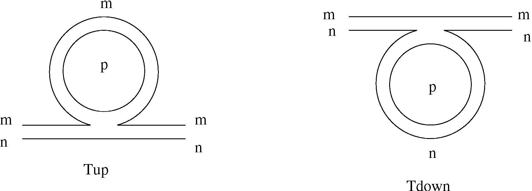
Figure 9: Two Point Graphs at one Loops: the up and down tadpoles

To compute $a$ we should add the wave function renormalization for the two tadpoles $T\ up$ and $T\ down$ of Figure 9. These two graphs have both a coupling constant $-\lambda/2$, and a combinatorial factor 2 for choosing to which leg of the vertex the external $\bar{\phi}$ contracts. Then the logarithmic divergence of $T\ up$ is

$$\sum_{p}(\frac{1}{m+p+A}-\frac{1}{p+A})=-\sum_{p}[\frac{m}{(m+p+A)(p+A)}]$$ (5.6)

so it corresponds to the renormalization of the coefficient of the $m$ factor in $G_{m,n}$ in 5.1, with logarithmic divergence $\lambda\sum_{p}[\frac{1}{p^{2}}]$. Similarly the logarithmic divergence of $T\ down$ gives the same renormalization but for the $n$ factor in $G_{m,n}$ in 5.1.

Altogether we find therefore that

$$a=+\sum_{p}[\frac{1}{p^{2}}]$$ (5.7)

In the real case we have a combinatoric factor $4$ instead of 2, but the coupling constant is $\lambda/4$, so $a$ is the same.

Figure 10: Four Point Graph at one Loop

The four point function perturbative expansion at one loop is

$$\Gamma_{4}(0,0,0,0)=-\lambda[1-a^{\prime}\lambda].$$ (5.8)

Only the graph B1 of Figure 10) contributes to $a^{\prime}$. It has a prefactor $\frac{1}{2!}(\lambda/2)^{2}$ and a combinatoric factor $2^{4}$ for contractions, since there is a factor 2 to choose whether the bubble is ”vertical or horizontal” ie if the horizontal bubble of Figure 10) is of $\bar{\phi}\star\phi\ \star\bar{\phi}\star\phi$ or of $\bar{\phi}\star\phi\ \star\bar{\phi}\star\phi$ type, then a factor 2 to choose to which vertex the first external; $\bar{\phi}$ contracts, then a factor 2 for the leg to which it contracts in that vertex and finally another factor 2 for the leg to which the other external $\bar{\phi}$ contracts.

The corresponding sum gives

$$a^{\prime}=(2^{4}\lambda/8)\sum_{p}\tfrac{1}{p^{2}}=2a\qquad(B1)\ .$$ (5.9)

so that at one loop equation 5.4 holds. In the real case we have a combinatoric factor $4^{3}$ instead of $2^{4}$, but the coupling constant is $\lambda/4$, so $a$ is the same and 5.4 holds.

Figure 11: Four Point Graphs at two Loops

5.2 Two and Three Loops

This computation was extended to two and three loops in [57]. The results were given in the form of tables for the discrete divergent sums and combinatoric weights of all planar regular graphs which appears at two and three loops in $\Gamma_{4}$ and $Z$. The equation 5.4 holds again, both in the real and complex cases.

Here we simply reproduce the list of contributing Feynman graphs. Indeed it is interesting to notice that although at large order there are less planar regular graphs than the general graphs of the commutative theory, the effect is opposite at small orders.

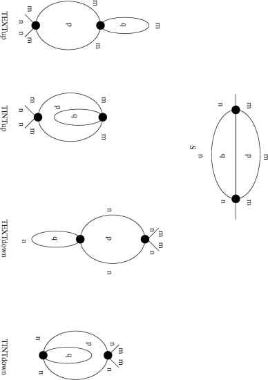
Figure 12: Two Point Graphs at Two Loops

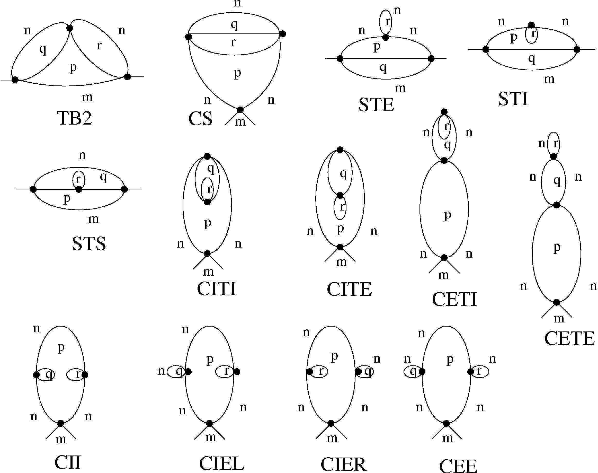
Figure 13: Two Point Graphs at Three Loops

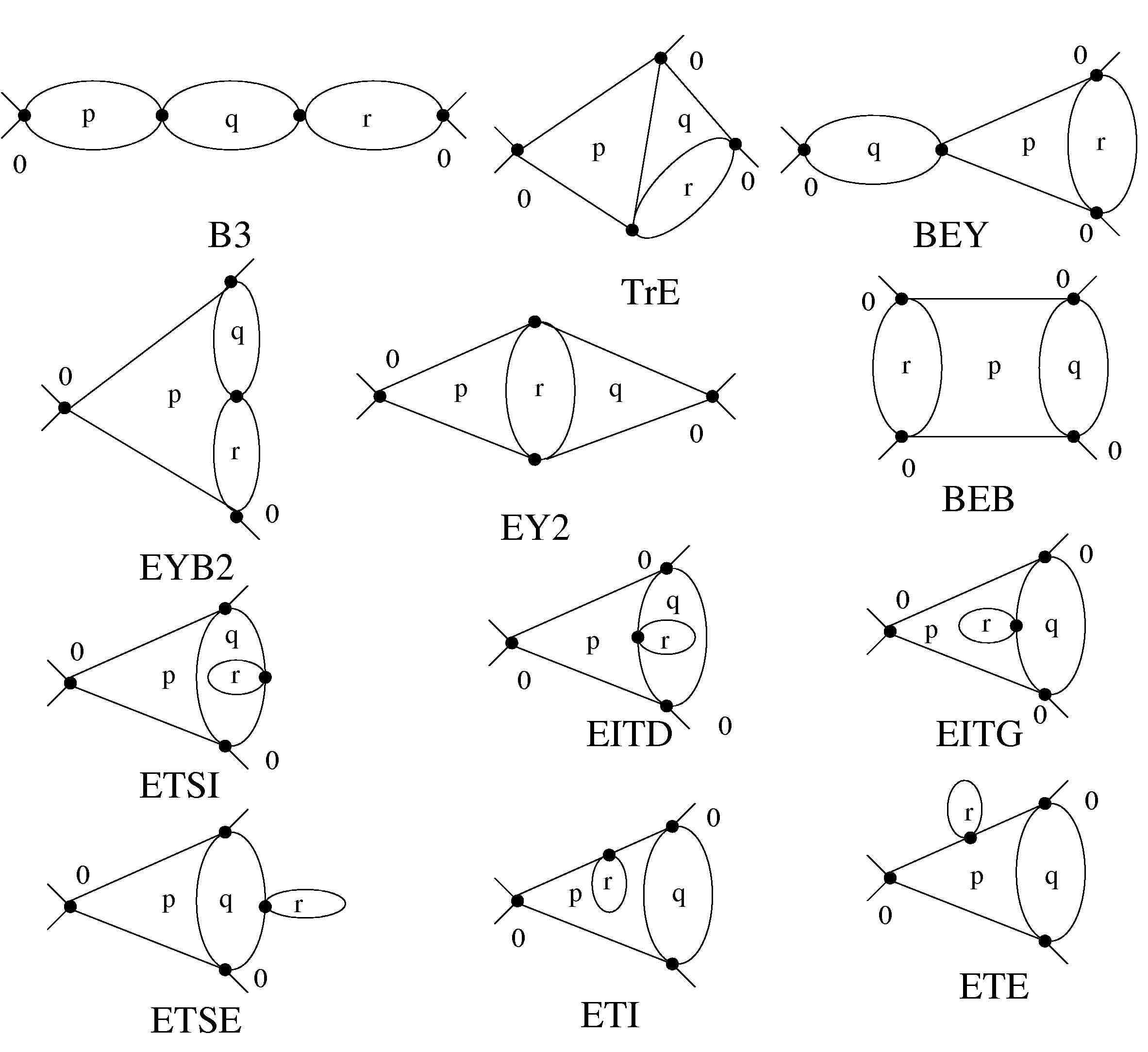
Figure 14: Four Point Graphs at Three Loops, Part I

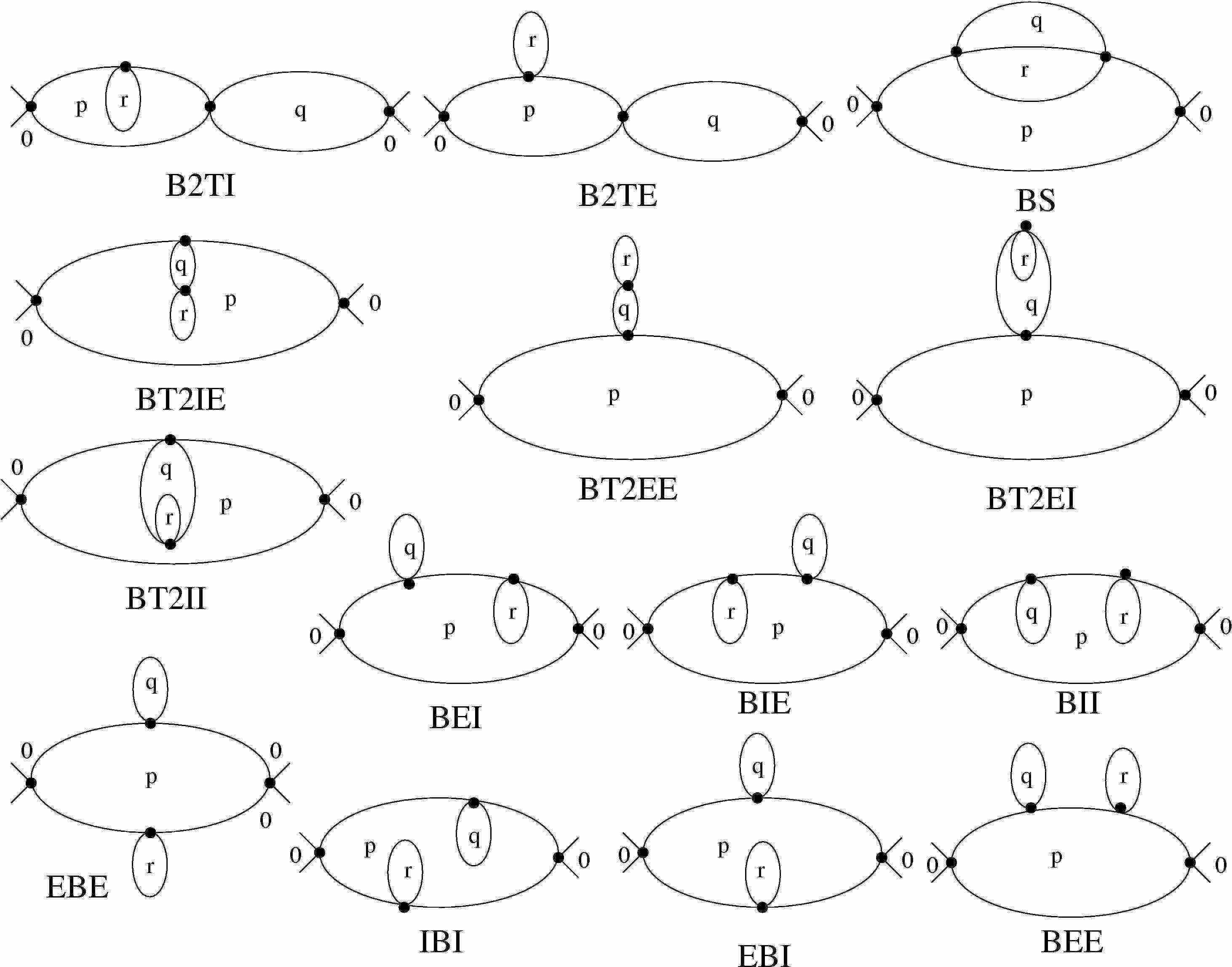
Figure 15: Four Point Graphs at Three Loops, Part II

5.3 The General Ward Identity

In this section, essentially reproduced from [58], we prove a general Ward identity which allows to check that theorem 5.1 continue to hold at any order in perturbation theory.

We orient the propagators from a $\bar{\phi}$ to a $\phi$. For a field $\bar{\phi}_{ab}$ we call the index $a$ a left index and the index, $b$ a right index. The first (second) index of a $\bar{\phi}$ always contracts with the second (first) index of a $\phi$. Consequently for $\phi_{cd}$, $c$ is a right index and $d$ is a left index.

Let $U=e^{\imath B}$ with $B$ a small hermitian matrix. We consider the “left” (as it acts only on the left indices) change of variables:

$$\phi^{U}=\phi U;\bar{\phi}^{U}=U^{\dagger}\bar{\phi}\ .$$ (5.10)

There is a similar “right” change of variables. The variation of the action is, at first order:

$$\delta S = \phi UXU^{\dagger}\bar{\phi}-\phi X\bar{\phi}\approx\imath\big{(}\phi BX\bar{\phi}-\phi XB\bar{\phi}\big{)}$$ (5.11)

$$= \imath B\big{(}X\bar{\phi}\phi-\bar{\phi}\phi X\big{)}$$

and the variation of the external sources is:

$$\delta F = U^{\dagger}\bar{\phi}\eta-\bar{\phi}\eta+\bar{\eta}\phi U-\bar{\eta}\phi\approx-\imath B\bar{\phi}\eta+\imath\bar{\eta}\phi B$$ (5.12)

$$= \imath B\big{(}-\bar{\phi}\eta+\bar{\eta}\phi{)}.$$

We obviously have:

$$\frac{\delta\ln Z}{\delta B_{ba}}=0=\frac{1}{Z(\bar{\eta},\eta)}\int d\bar{\phi}d\phi\big{(}-\frac{\delta S}{\delta B_{ba}}+\frac{\delta F}{\delta B_{ba}}\big{)}e^{-S+F}$$

$$=\frac{1}{Z(\bar{\eta},\eta)}\int d\bar{\phi}d\phi\leavevmode\nobreak\ e^{-S+F}\big{(}-[X\bar{\phi}\phi-\bar{\phi}\phi X]_{ab}+[-\bar{\phi}\eta+\bar{\eta}\phi]_{ab}\big{)}\ .$$ (5.13)

We now apply $\partial_{\eta}\partial_{\bar{\eta}}|_{\eta=\bar{\eta}=0}$ on the above expression. As we have at most two insertions, we get only the connected components of the correlation functions.

$$0=<\partial_{\eta}\partial_{\bar{\eta}}\big{(}-[X\bar{\phi}\phi-\bar{\phi}\phi X]_{ab}+[-\bar{\phi}\eta+\bar{\eta}\phi]_{ab}\big{)}e^{F(\bar{\eta},\eta)}|_{0}>_{c}\ ,$$ (5.14)

which gives:

$$<\frac{\partial(\bar{\eta}\phi)_{ab}}{\partial\bar{\eta}}\frac{\partial(\bar{\phi}\eta)}{\partial\eta}-\frac{\partial(\bar{\phi}\eta)_{ab}}{\partial\eta}\frac{\partial(\bar{\eta}\phi)}{\partial\bar{\eta}}-[X\bar{\phi}\phi-\bar{\phi}\phi X]_{ab}\frac{\partial(\bar{\eta}\phi)}{\partial\bar{\eta}}\frac{\partial(\bar{\phi}\eta)}{\partial\eta}>_{c}=0.$$ (5.15)

Using the explicit form of $X$ we get:

$$(a-b)<[\bar{\phi}\phi]_{ab}\frac{\partial(\bar{\eta}\phi)}{\partial\bar{\eta}}\frac{\partial(\bar{\phi}\eta)}{\partial\eta}>_{c}=<\frac{\partial(\bar{\eta}\phi)_{ab}}{\partial\bar{\eta}}\frac{\partial(\bar{\phi}\eta)}{\partial\eta}>_{c}-<\frac{\partial(\bar{\phi}\eta)_{ab}}{\partial\eta}\frac{\partial(\bar{\eta}\phi)}{\partial\bar{\eta}}>\ ,$$

and for $\bar{\eta}_{\beta\alpha}\eta_{\nu\mu}$ we get:

$$(a-b)<[\bar{\phi}\phi]_{ab}\phi_{\alpha\beta}\bar{\phi}_{\mu\nu}>_{c}=<\delta_{a\beta}\phi_{\alpha b}\bar{\phi}_{\mu\nu}>_{c}-<\delta_{b\mu}\bar{\phi}_{a\nu}\phi_{\alpha\beta}>_{c}$$ (5.16)

We restrict to terms in the above expressions which are planar with a single external face, as all others are irrelevant. Such terms have $\alpha=\nu$, $a=\beta$ and $b=\mu$. The Ward identity for the $2$ point function reads:

$$(a-b)<[\bar{\phi}\phi]_{ab}\phi_{\nu a}\bar{\phi}_{b\nu}>_{c}=<\phi_{\nu b}\bar{\phi}_{b\nu}>_{c}-<\bar{\phi}_{a\nu}\phi_{\nu a}>_{c}$$ (5.17)

(repeated indices are not summed).

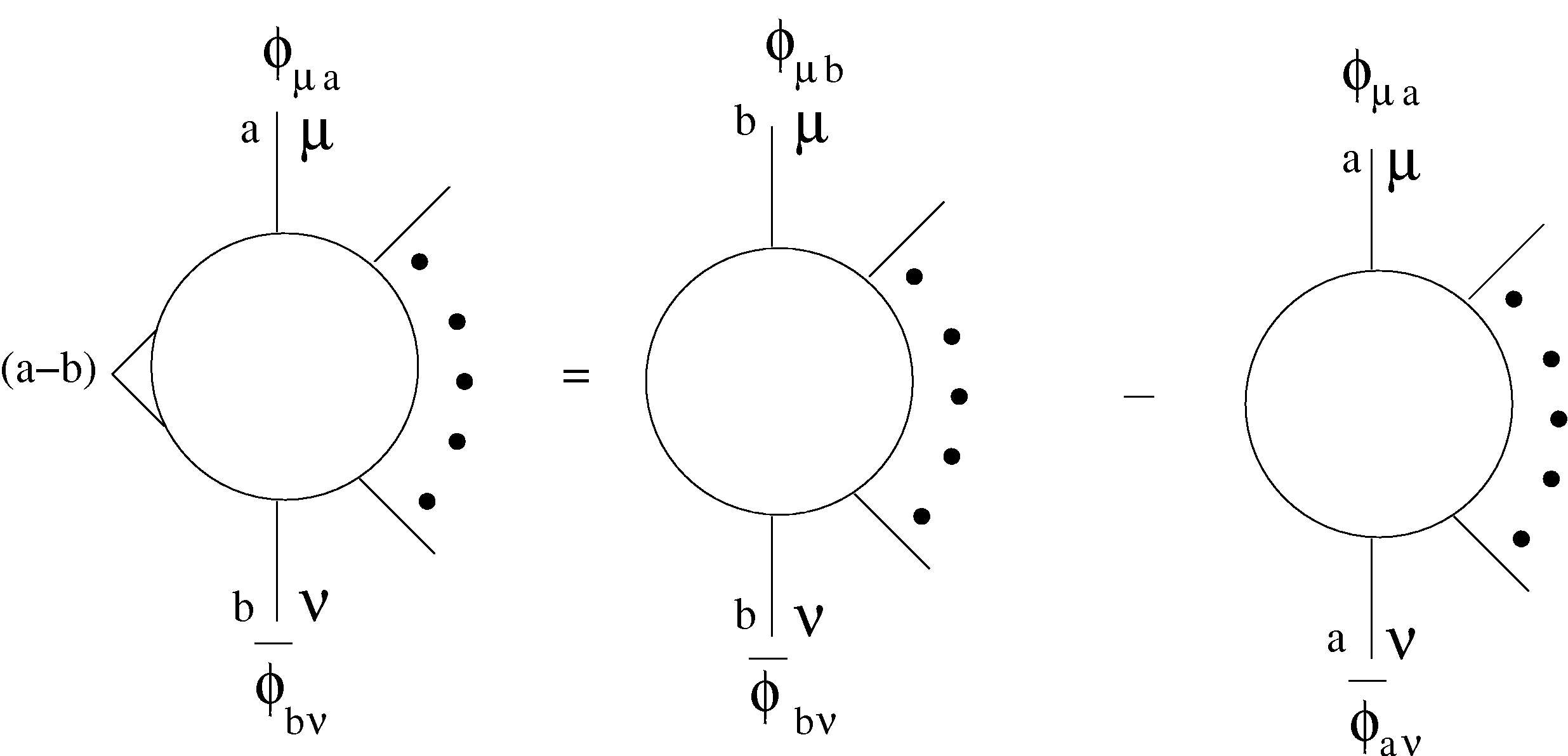
Figure 16: The Ward identity for a 2p point function with insertion on the left face

Derivating further we get:

$$(a-b)<[\bar{\phi}\phi]_{ab}\partial_{\bar{\eta}_{1}}(\bar{\eta}\phi)\partial_{\eta_{1}}(\bar{\phi}\eta)\partial_{\bar{\eta}_{2}}(\bar{\eta}\phi)\partial_{\eta_{2}}(\bar{\phi}\eta)>_{c}=$$ (5.18)

$$<\partial_{\bar{\eta}_{1}}(\bar{\eta}\phi)\partial_{\eta_{1}}(\bar{\phi}\eta)\big{[}\partial_{\bar{\eta_{2}}}(\bar{\eta}\phi)_{ab}\partial_{\eta_{2}}(\bar{\phi}\eta)-\partial_{\eta_{2}}(\bar{\phi}\eta)_{ab}\partial_{\bar{\eta}_{2}}(\bar{\eta}\phi)\big{]}>_{c}+1\leftrightarrow 2\ .$$

Take $\bar{\eta}_{1\leavevmode\nobreak\ \beta\alpha}$, $\eta_{1\leavevmode\nobreak\ \nu\mu}$, $\bar{\eta}_{2\leavevmode\nobreak\ \delta\gamma}$ and $\eta_{2\leavevmode\nobreak\ \sigma\rho}$. We get:

$$(a-b)<[\bar{\phi}\phi]_{ab}\phi_{\alpha\beta}\bar{\phi}_{\mu\nu}\phi_{\gamma\delta}\bar{\phi}_{\rho\sigma}>_{c}$$ (5.19)

$$=<\phi_{\alpha\beta}\bar{\phi}_{\mu\nu}\delta_{a\delta}\phi_{\gamma b}\bar{\phi}_{\rho\sigma}>_{c}-<\phi_{\alpha\beta}\bar{\phi}_{\mu\nu}\phi_{\gamma\delta}\bar{\phi}_{a\sigma}\delta_{b\rho}>_{c}+$$

$$<\phi_{\gamma\delta}\bar{\phi}_{\rho\sigma}\delta_{a\beta}\phi_{\alpha b}\bar{\phi}_{\mu\nu}>_{c}-<\phi_{\gamma\delta}\bar{\phi}_{\rho\sigma}\phi_{\alpha\beta}\bar{\phi}_{a\nu}\delta_{b\mu}>_{c}\ .$$

Again neglecting all terms which are not planar with a single external face leads to

$$(a-b)<\phi_{\alpha a}[\bar{\phi}\phi]_{ab}\bar{\phi}_{b\nu}\phi_{\nu\delta}\bar{\phi}_{\delta\alpha}>_{c}=<\phi_{\alpha b}\bar{\phi}_{b\nu}\phi_{\nu\delta}\bar{\phi}_{\delta\alpha}>_{c}-<\phi_{\alpha a}\bar{\phi}_{a\nu}\phi_{\nu\delta}\bar{\phi}_{\delta\alpha}>_{c}\ .$$

Clearly there are similar identities for $2p$ point functions for any $p$.

The indices $a$ and $b$ are left indices, so that we have the Ward identity with an insertion on a left face as represented in Fig. 16. There is a similar Ward identity obtained with the “right” transformation, consequently with the insertion on a right face.

5.3.1 Proof of Theorem 5.1

We start this section by some definitions: we will denote $G^{4}(m,n,k,l)$ the connected four point function restricted to the planar one broken face case, where $m,n,k,l$ are the indices of the external face in the correct cyclic order. The first index $m$ always represents a left index.

Similarly, $G^{2}(m,n)$ is the connected planar one broken face two point function with $m,n$ the indices on the external face (also called the dressed propagator, see Fig. 17). $G^{2}(m,n)$ and $\Sigma(m,n)$ are related by:

$$G^{2}(m,n)=\frac{C_{mn}}{1-C_{mn}\Sigma(m,n)}=\frac{1}{C_{mn}^{-1}-\Sigma(m,n)}\,.$$ (5.20)

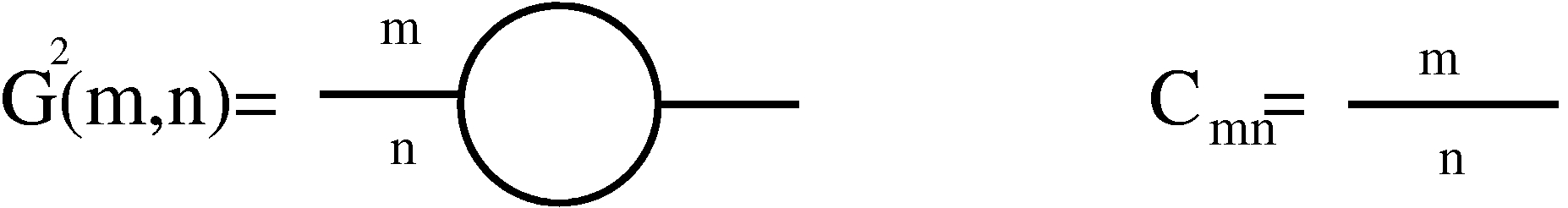
Figure 17: The dressed and the bare propagators

$G_{ins}(a,b;...)$ will denote the planar one broken face connected function with one insertion on the left border where the matrix index jumps from $a$ to $b$. With this notations the Ward identity (5.17) writes:

$$(a-b)\leavevmode\nobreak\ G^{2}_{ins}(a,b;\nu)=G^{2}(b,\nu)-G^{2}(a,\nu)\,.$$ (5.21)

All the identities we use, either Ward identities or the Dyson equation of motion can be written either for the bare theory or for the theory with complete mass renormalization, which is the one considered in [57]. In the first case the parameter $A$ in (5.1) is the bare one, $A_{bare}$ and there is no mass subtraction. In the second case the parameter $A$ in (5.1) is $A_{ren}=A_{bare}-\Sigma(0,0)$, and every two point 1PI subgraph is subtracted at 0 external indices. $\partial_{L}$ denotes the derivative with respect to a left index and $\partial_{R}$ the one with respect to a right index. When the two derivatives are equal we use the generic notation $\partial$.

Let us prove first the Theorem in the mass-renormalized case, then in the next subsection in the bare case. Indeed the mass renormalized theory used is free from any quadratic divergences. Remaining logarithmic subdivergences in the ultra violet cutoff can be removed easily by passing to the effective series as explained in [57].

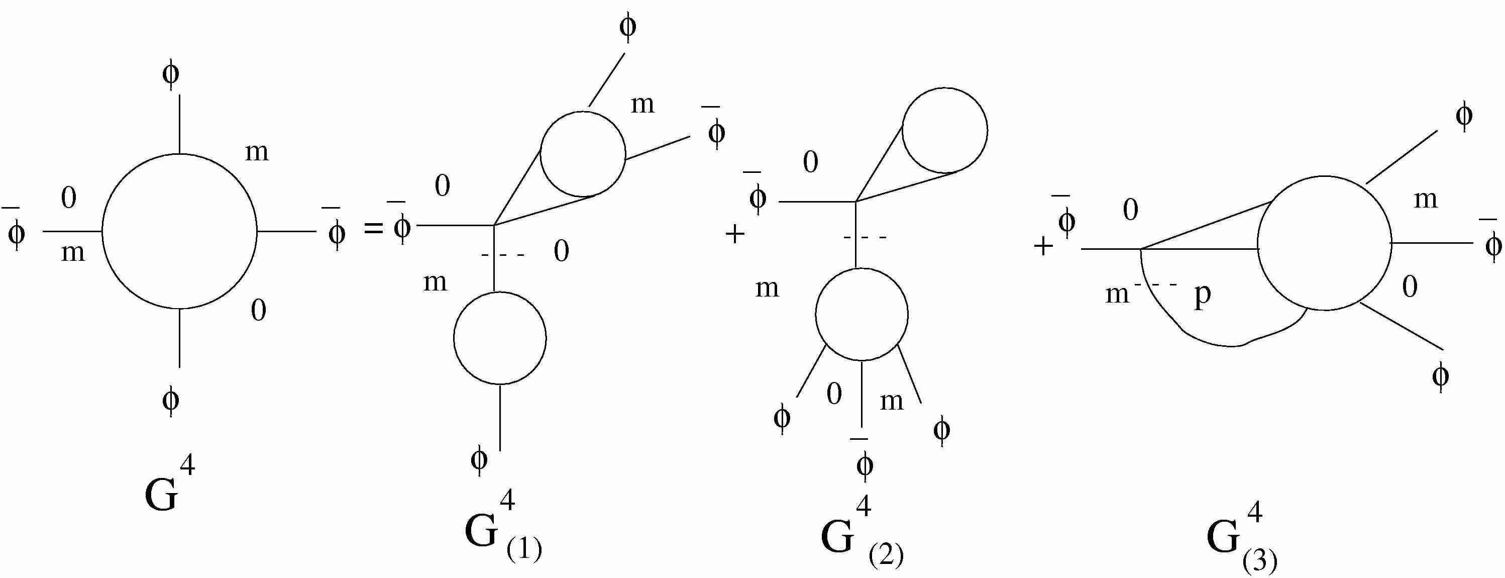
Figure 18: The Dyson equation

We analyze a four point connected function $G^{4}(0,m,0,m)$ with index $m\neq 0$ on the right borders. This explicit break of left-right symmetry is adapted to our problem.

Consider a $\bar{\phi}$ external line and the first vertex hooked to it. Turning right on the $m$ border at this vertex we meet a new line (the slashed line in Fig. 18). The slashed line either separates the graph into two disconnected components ($G^{4}_{(1)}$ and $G^{4}_{(2)}$ in Fig. 18) or not ($G^{4}_{(3)}$ in Fig. 18). Furthermore, if the slashed line separates the graph into two disconnected components the first vertex may either belong to the four point component ($G^{4}_{(1)}$ in Fig. 18) or to the two point component ($G^{4}_{(2)}$ in Fig. 18).

We stress that this is a classification of graphs: the different components depicted in Fig. 18 take into account all the combinatoric factors. Furthermore, the setting of the external indices to $0$ on the left borders and $m$ on the right borders distinguishes the $G^{4}_{(1)}$ and $G^{4}_{(2)}$ from their counterparts “pointing upwards”: indeed, the latter are classified in $G^{4}_{(3)}$!

We have thus the Dyson equation:

$$G^{4}(0,m,0,m)=G^{4}_{(1)}(0,m,0,m)+G^{4}_{(2)}(0,m,0,m)+G^{4}_{(3)}(0,m,0,m)\,.$$ (5.22)

The second term, $G^{4}_{(2)}$, is zero. Indeed the mass renormalized two point insertion is zero, as it has the external left index set to zero. Note that this is an insertion exclusively on the left border. The simplest case of such an insertion is a (left) tadpole. We will (naturally) call a general insertion touching only the left border a “generalized left tadpole”.

We will prove that $G^{4}_{(1)}+G^{4}_{(3)}$ yields $\Gamma^{4}=\lambda(1-\partial\Sigma)^{2}$ after amputation of the four external propagators.

We start with $G^{4}_{(1)}$. It is of the form:

$$G^{4}_{(1)}(0,m,0,m)=\lambda C_{0m}G^{2}(0,m)G^{2}_{ins}(0,0;m)\,.$$ (5.23)

By the Ward identity we have:

$$G^{2}_{ins}(0,0;m) = \lim_{\zeta\rightarrow 0}G^{2}_{ins}(\zeta,0;m)=\lim_{\zeta\rightarrow 0}\frac{G^{2}(0,m)-G^{2}(\zeta,m)}{\zeta}$$ (5.24)

$$= -\partial_{L}G^{2}(0,m)\,.$$

Using the explicit form of the bare propagator we have $\partial_{L}C^{-1}_{ab}=\partial_{R}C^{-1}_{ab}=\partial C^{-1}_{ab}=1$. Reexpressing $G^{2}(0,m)$ by eq. (5.20) we conclude that:

$$G^{4}_{(1)}(0,m,0,m) = \lambda C_{0m}\frac{C_{0m}C^{2}_{0m}[1-\partial_{L}\Sigma(0,m)]}{[1-C_{0m}\Sigma(0,m)](1-C_{0m}\Sigma(0,m))^{2}}$$ (5.25)

$$= \lambda[G^{2}(0,m)]^{4}\frac{C_{0m}}{G^{2}(0,m)}[1-\partial_{L}\Sigma(0,m)]\,.$$

The self energy is (again up to irrelevant terms ([40]):

$$\Sigma(m,n)=\Sigma(0,0)+(m+n)\partial\Sigma(0,0)$$ (5.26)

Therefore up to irrelevant terms ($C^{-1}_{0m}=m+A_{ren}$) we have:

$$G^{2}(0,m)=\frac{1}{m+A_{bare}-\Sigma(0,m)}=\frac{1}{m[1-\partial\Sigma(0,0)]+A_{ren}}\,,$$ (5.27)

and

$$\frac{C_{0m}}{G^{2}(0,m)}=1-\partial\Sigma(0,0)+\frac{A_{ren}}{m+A_{ren}}\partial\Sigma(0,0)\,.$$ (5.28)

Inserting eq. (5.28) in eq. (5.25) holds:

$$G^{4}_{(1)}(0,m,0,m) = \lambda[G^{2}(0,m)]^{4}\bigl{(}1-\partial\Sigma(0,0)+\frac{A_{ren}}{m+A_{ren}}\partial\Sigma(0,0)\bigr{)}$$ (5.29)

$$[1-\partial_{L}\Sigma(0,m)]\,.$$

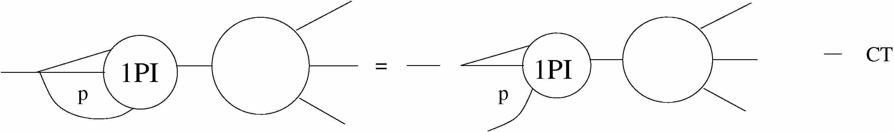
Figure 19: Two point insertion and opening of the loop with index $p$

For the $G^{4}_{(3)}(0,m,0,m)$ one starts by “opening” the face which is “first on the right”. The summed index of this face is called $p$ (see Fig. 18). For bare Green functions this reads:

$$G^{4,bare}_{(3)}(0,m,0,m)=C_{0m}\sum_{p}G^{4,bare}_{ins}(p,0;m,0,m)\,.$$ (5.30)

When passing to mass renormalized Green functions one must be cautious. It is possible that the face $p$ belonged to a 1PI two point insertion in $G^{4}_{(3)}$ (see the left hand side in Fig. 19). Upon opening the face $p$ this 2 point insertion disappears (see right hand side of Fig. 19)! When renormalizing, the counterterm coresponding to this kind of two point insertion will be subtracted on the left hand side of eq.(5.30), but not on the right hand side. In the equation for $G^{4}_{(3)}(0,m,0,m)$ one must therefore add its missing counterterm, so that:

$$G^{4}_{(3)}(0,m,0,m) = C_{0m}\sum_{p}G^{4}_{ins}(0,p;m,0,m)$$ (5.31)

$$- C_{0m}(CT_{lost})G^{4}(0,m,0,m)\,.$$

It is clear that not all 1PI 2 point insertions on the left hand side of Fig. 19 will be “lost” on the right hand side. If the insertion is a “generalized left tadpole” it is not “lost” by opening the face $p$ (imagine a tadpole pointing upwards in Fig.19: clearly it will not be opened by opening the line). We will call the 2 point 1PI insertions “lost” on the right hand side $\Sigma^{R}(m,n)$. Denoting the generalized left tadpole $T^{L}$ we can write (see Fig .20):

$$\Sigma(m,n)=T^{L}(m,n)+\Sigma^{R}(m,n)\,.$$ (5.32)

Note that as $T^{L}(m,n)$ is an insertion exclusively on the left border, it does not depend upon the right index $n$. We therefore have $\partial\Sigma(m,n)=\partial_{R}\Sigma(m,n)=\partial_{R}\Sigma^{R}(m,n)$.

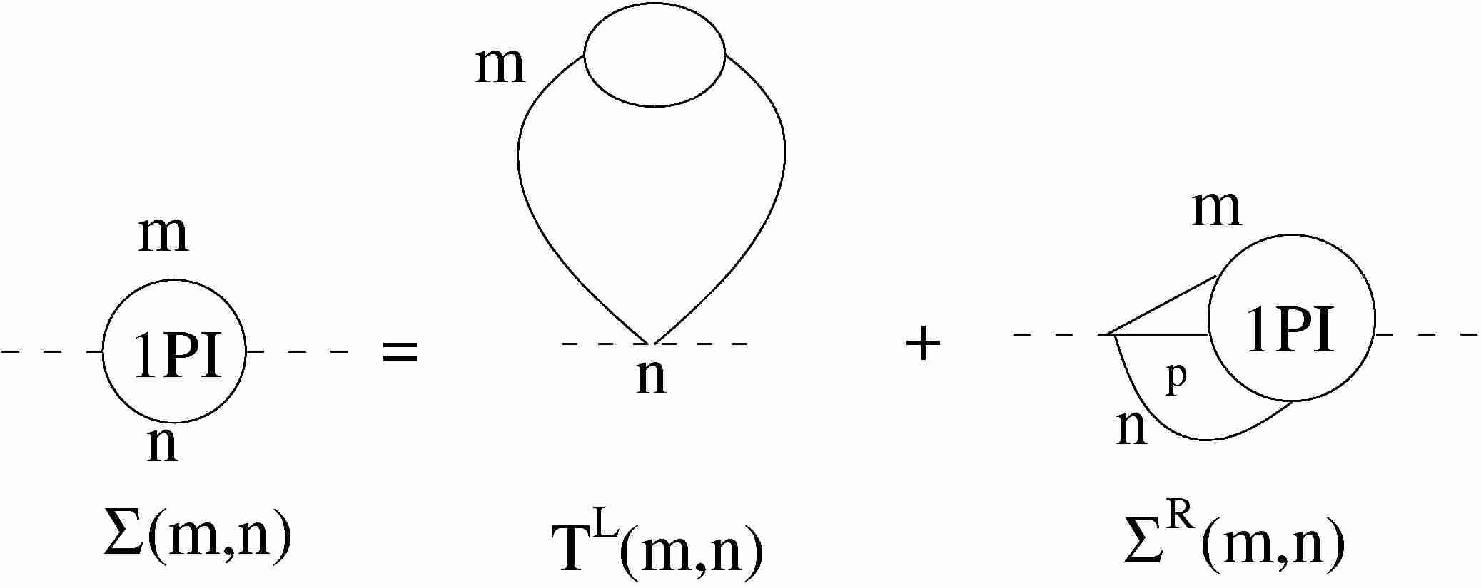
Figure 20: The self energy

The missing mass counterterm writes:

$$CT_{lost}=\Sigma^{R}(0,0)=\Sigma(0,0)-T^{L}\,.$$ (5.33)

In order to evaluate $\Sigma^{R}(0,0)$ we procede by opening its face $p$ and using the Ward identity (5.17), to obtain:

$$\Sigma^{R}(0,0) = \frac{1}{G^{2}(0,0)}\sum_{p}G^{2}_{ins}(0,p;0)$$ (5.34)

$$= \frac{1}{G^{2}(0,0)}\sum_{p}\frac{1}{p}[G^{2}(0,0)-G^{2}(p,0)]$$

$$= \sum_{p}\frac{1}{p}\biggl{(}1-\frac{G^{2}(p,0)}{G^{2}(0,0)}\biggr{)}\,.$$

Using eq. (5.31) and eq. (5.34) we have:

$$G^{4}_{(3)}(0,m,0,m) = C_{0m}\sum_{p}G^{4}_{ins}(0,p;m,0,m)$$ (5.35)

$$- C_{0m}G^{4}(0,m,0,m)\sum_{p}\frac{1}{p}\biggl{(}1-\frac{G^{2}(p,0)}{G^{2}(0,0)}\biggr{)}\,.$$

But by the Ward identity (5.3):

$$C_{0m}\sum_{p}G^{4}_{ins}(0,p;m,0,m)=C_{0m}\sum_{p}\frac{1}{p}\biggl{(}G^{4}(0,m,0,m)-G^{4}(p,m,0,m)\biggr{)}\,,$$ (5.36)

The second term in eq. (5.36), having at least three denominators linear in $p$, is irrelevant . Substituting eq. (5.36) in eq . (5.35) we have:

$$G^{4}_{(3)}(0,m,0,m)=C_{0m}\frac{G^{4}(0,m,0,m)}{G^{2}(0,0)}\sum_{p}\frac{G^{2}(p,0)}{p}\,.$$ (5.37)

To conclude we must evaluate the sum in eq. (5.37). Using eq. (5.27) we have:

$$\sum_{p}\frac{G^{2}(p,0)}{p}=\sum_{p}\frac{G^{2}(p,0)}{p}\bigl{(}\frac{1}{G^{2}(0,1)}-\frac{1}{G^{2}(0,0)}\bigr{)}\frac{1}{1-\partial\Sigma(0,0)}$$ (5.38)

In order to interpret the two terms in the above equation we start by performing the same manipulations as in eq (5.34) for $\Sigma^{R}(0,1)$. We get:

$$\Sigma^{R}(0,1) = \sum_{p}\frac{1}{p}\biggl{(}1-\frac{G^{2}(p,1)}{G^{2}(0,1)}\biggr{)}=\sum_{p}\frac{1}{p}\biggl{(}1-\frac{G^{2}(p,0)}{G^{2}(0,1)}\biggr{)}\,.$$ (5.39)

where in the second equality we have neglected an irrelevant term.

Substituting eq. (5.34) and eq. (5.39) in eq. (5.38) we get:

$$\sum_{p}\frac{G^{2}(p,0)}{p}=\frac{\Sigma^{R}(0,0)-\Sigma^{R}(0,1)}{1-\partial\Sigma(0,0)}=-\frac{\partial_{R}\Sigma^{R}(0,0)}{1-\partial\Sigma(0,0)}=-\frac{\partial\Sigma(0,0)}{1-\partial\Sigma(0,0)}\,.$$ (5.40)

as $\partial_{R}\Sigma^{R}=\partial\Sigma$. Hence:

$$G^{4}_{(3)}(0,m,0,m;p) = -C_{0m}G^{4}(0,m,0,m)\frac{1}{G^{2}(0,0)}\frac{\partial\Sigma(0,0)}{1-\partial\Sigma(0,0)}$$ (5.41)

$$= -G^{4}(0,m,0,m)\frac{A_{ren}\;\partial\Sigma(0,0)}{(m+A_{ren})[1-\partial\Sigma(0,0)]}\ .$$

Using (5.29) and (5.41), equation (5.22) rewrites as:

$$G^{4}(0,m,0,m)\Big{(}1+\frac{A_{ren}\;\partial\Sigma(0,0)}{(m+A_{ren})\;[1-\partial\Sigma(0,0)]}\Big{)}$$ (5.42)

$$=\lambda_{bare}(G^{2}(0,m))^{4}\Big{(}1-\partial\Sigma(0,0)+\frac{A_{ren}}{m+A_{ren}}\partial\Sigma(0,0)\Big{)}[1-\partial_{L}\Sigma(0,m)]\,.$$

We multiply (5.42) by $[1-\partial\Sigma(0,0)]$ and amputate four times. As the differences $\Gamma^{4}(0,m,0,m,)-\Gamma^{4}(0,0,0,0)$ and $\partial_{L}\Sigma(0,m)-\partial_{L}\Sigma(0,0)$ are irrelevant we get:

$$\Gamma^{4}(0,0,0,0)=\lambda(1-\partial\Sigma(0,0))^{2}\,.$$ (5.43)

∎

5.3.2 Bare identity

Let us explain now why the main theorem is also true as an identity between bare functions, without any renormalization, but with ultraviolet cutoff.

Using the same Ward identities, all the equations go through with only few differences:

- we should no longer add the lost mass counterterm in (5.33)

- the term $G^{4}_{(2)}$ is no longer zero.

- equation (5.28) and all propagators now involve the bare $A$ parameter.

But these effects compensate. Indeed the bare $G^{4}_{(2)}$ term is the left generalized tadpole $\Sigma-\Sigma^{R}$, hence

$$G^{4}_{(2)}(0,m,0,m)=C_{0,m}\bigl{(}\Sigma(0,m)-\Sigma^{R}(0,m)\bigr{)}G^{4}(0,m,0,m)\;.$$ (5.44)

Equation (5.28) becomes up to irrelevant terms

$$\frac{C^{bare}_{0m}}{G^{2,bare}(0,m)}=1-\partial_{L}\Sigma(0,0)+\frac{A_{bare}}{m+A_{bare}}\partial_{L}\Sigma(0,0)-\frac{1}{m+A_{bare}}\Sigma(0,0)$$ (5.45)

The first term proportional to $\Sigma(0,m)$ in (5.44) combines with the new term in (5.45), and the second term proportional to $\Sigma^{R}(0,m)$ in (5.44) is exactly the former “lost counterterm” (5.33). This proves (5.4) in the bare case.

5.4 The RG Flow

It remains to understand better the meaning of the Langmann-Szabo symmetry which certainly lies behind this Ward identity. Of course we also need to develop a non-perturbative or constructive analysis of the theory to fully confirm the absence of the Landau ghost. If this constructive analysis confirms the perturbative picture the expected non perturbative flow for the effective parameters $\lambda$ and $\Omega$ should be:

$$\frac{d\lambda_{i}}{di} \simeq a(1-\Omega_{i})F(\lambda_{i})\ ,$$ (5.46)

$$\frac{d\Omega_{i}}{di} \simeq b(1-\Omega_{i})G(\lambda_{i})\ ,$$ (5.47)

where $F(\lambda_{i})=\lambda_{i}^{2}+O(\lambda_{i}^{3})$, $G(\lambda_{i})=\lambda_{i}+O(\lambda_{i}^{2})$ and $a,b\in\mathbb{R}$ are two constants. The behavior of this system is qualitatively the same as the simpler system

$$\frac{d\lambda_{i}}{di} \simeq a(1-\Omega_{i})\lambda_{i}^{2}\ ,$$ (5.48)

$$\frac{d\Omega_{i}}{di} \simeq b(1-\Omega_{i})\lambda_{i}\ ,$$ (5.49)

whose solution is

$$\lambda_{i}=\lambda_{0}e^{\frac{a}{b}(\Omega_{i}-\Omega_{0})}\ ,$$ (5.50)

with $\Omega_{i}$ solution of

$$b\;i\;\lambda_{0}=\int_{1-\Omega_{i}}^{1-\Omega_{0}}e^{\frac{au}{b}}\frac{du}{u}\ ,$$ (5.51)

hence going exponentially fast to 1 as $i$ goes to infinity. The corresponding numerical flow is drawn on Figure 21.

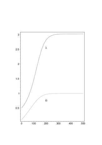
Figure 21: Numerical flow for $\lambda$ and $\Omega$

Of course to establish fully rigorously this picture is beyond the reach of perturbative theorems and requires a constructive analysis.

6 Propagators on non-commutative space

We give here the results we get in [50]. In this article, we computed the $x$-space and matrix basis kernels of operators which generalize the Mehler kernel (3.34). Then we proceeded to a study of the scaling behaviors of these kernels in the matrix basis. This work is useful to study the non-commutative Gross-Neveu model in the matrix basis.

6.1 Bosonic kernel

The following lemma generalizes the Mehler kernel [91]:

Lemma 6.1.

Let $H$ the operator:

$$H=\frac{1}{2}\Big{(}-\Delta+\Omega^{2}x^{2}-2\imath B(x_{0}\partial_{1}-x_{1}\partial_{0})\Big{)}.$$ (6.1)

The $x$-space kernel of $e^{-tH}$ is:

$$e^{-tH}(x,x^{\prime})=\frac{\Omega}{2\pi\sinh\Omega t}e^{-A},$$ (6.2)

$$A=\frac{\Omega\cosh\Omega t}{2\sinh\Omega t}(x^{2}+x^{\prime 2})-\frac{\Omega\cosh Bt}{\sinh\Omega t}x\cdot x^{\prime}-\imath\frac{\Omega\sinh Bt}{\sinh\Omega t}x\wedge x^{\prime}.$$ (6.3)

Remark.

The Mehler kernel corresponds to $B=0$. The limit $\Omega=B\to 0$ gives the usual heat kernel.

Lemma 6.2.

Let $H$ be given by (6.1) with $\Omega(B)\to 2\Omega/\theta(2B\theta)$. Its inverse in the matrix basis is:

$$H^{-1}_{m,m+h;l+h,l}=\frac{\theta}{8\Omega}\int_{0}^{1}d\alpha\,\dfrac{(1-\alpha)^{\frac{\mu_{0}^{2}\theta}{8\Omega}+(\frac{D}{4}-1)}}{(1+C\alpha)^{\frac{D}{2}}}(1-\alpha)^{-\frac{4B}{8\Omega}h}\prod_{s=1}^{\frac{D}{2}}G^{(\alpha)}_{m^{s},m^{s}+h^{s};l^{s}+h^{s},l^{s}},$$ (6.4)

$$G^{(\alpha)}_{m,m+h;l+h,l}=\left(\frac{\sqrt{1-\alpha}}{1+C\alpha}\right)^{m+l+h}\sum_{u=\max(0,-h)}^{\min(m,l)}{\mathcal{A}}(m,l,h,u)\left(\frac{C\alpha(1+\Omega)}{\sqrt{1-\alpha}(1-\Omega)}\right)^{m+l-2u},$$

where ${\mathcal{A}}(m,l,h,u)=\sqrt{\binom{m}{m-u}\binom{m+h}{m-u}\binom{l}{l-u}\binom{l+h}{l-u}}$ and $C$ is a function of $\Omega$ : $C(\Omega)=\frac{(1-\Omega)^{2}}{4\Omega}$.

6.2 Fermionic kernel

On the Moyal space, we modified the commutative Gross-Neveu model by adding a $\not{\widetilde{x}}$ term (see lemma 3.4). We have

$$G(x,y) = -\frac{\Omega}{\theta\pi}\int_{0}^{\infty}\frac{dt}{\sinh(2\widetilde{\Omega}t)}\,e^{-\frac{\widetilde{\Omega}}{2}\coth(2\widetilde{\Omega}t)(x-y)^{2}+\imath\widetilde{\Omega}x\wedge y}$$

$$\left\{\imath\widetilde{\Omega}\coth(2\widetilde{\Omega}t)(\not{x}-\not{y})+\Omega(\not{\widetilde{x}}-\not{\widetilde{y}})-\mu\right\}e^{-2\imath\widetilde{\Omega}t\gamma^{0}\gamma^{1}}e^{-t\mu^{2}}\;.$$

It will be useful to express $G$ in terms of commutators:

$$G(x,y) = -\frac{\Omega}{\theta\pi}\int_{0}^{\infty}dt\,\left\{\imath\widetilde{\Omega}\coth(2\widetilde{\Omega}t)\left[\not{x},\Gamma^{t}\right](x,y)\right.$$ (6.6)

$$\left.+\Omega\left[\not{\widetilde{x}},\Gamma^{t}\right](x,y)-\mu\Gamma^{t}(x,y)\right\}e^{-2\imath\widetilde{\Omega}t\gamma^{0}\gamma^{1}}e^{-t\mu^{2}},$$

where

$$\Gamma^{t}(x,y) = \frac{1}{\sinh(2\widetilde{\Omega}t)}\,e^{-\frac{\widetilde{\Omega}}{2}\coth(2\widetilde{\Omega}t)(x-y)^{2}+\imath\widetilde{\Omega}x\wedge y}$$ (6.7)

with $\widetilde{\Omega}=\frac{2\Omega}{\theta}$ and $x\wedge y=x^{0}y^{1}-x^{1}y^{0}$.

We now give the expression of the Fermionic kernel (6.6) in the matrix basis. The inverse of the quadratic form

$$\Delta=p^{2}+\mu^{2}+\frac{4\Omega^{2}}{\theta^{2}}x^{2}+\frac{4B}{\theta}L_{2}$$ (6.8)

is given by (6.4) in the preceeding section:

$$\Gamma_{m,m+h;l+h,l} =\frac{\theta}{8\Omega}\int_{0}^{1}d\alpha\,\dfrac{(1-\alpha)^{\frac{\mu^{2}\theta}{8\Omega}-\frac{1}{2}}}{(1+C\alpha)}\Gamma^{\alpha}_{m,m+h;l+h,l}\,$$ (6.9)

$$\Gamma^{(\alpha)}_{m,m+h;l+h,l} =\left(\frac{\sqrt{1-\alpha}}{1+C\alpha}\right)^{m+l+h}\left(1-\alpha\right)^{-\frac{Bh}{2\Omega}}$$ (6.10)

$$\sum_{u=0}^{\min(m,l)}{\cal A}(m,l,h,u)\ \left(\frac{C\alpha(1+\Omega)}{\sqrt{1-\alpha}\,(1-\Omega)}\right)^{m+l-2u}.$$

The Fermionic propagator $G$ (6.6) in the matrix basis may be deduced from the kernel (6.9). We just set $B=\Omega$, add the missing term with $\gamma^{0}\gamma^{1}$ and compute the action of $-\not{p}-\Omega\not{\widetilde{x}}+\mu$ on $\Gamma$. We must then evaluate $\left[x^{\nu},\Gamma\right]$ in the matrix basis:

$$\left[x^{0},\Gamma\right]_{m,n;k,l}= 2\pi\theta\sqrt{\frac{\theta}{8}}\left\{\sqrt{m+1}\Gamma_{m+1,n;k,l}-\sqrt{l}\Gamma_{m,n;k,l-1}+\sqrt{m}\Gamma_{m-1,n;k,l}\right.$$

$$-\sqrt{l+1}\Gamma_{m,n;k,l+1}+\sqrt{n+1}\Gamma_{m,n+1;k,l}-\sqrt{k}\Gamma_{m,n;k-1,l}$$

$$\left.+\sqrt{n}\Gamma_{m,n-1;k,l}-\sqrt{k+1}\Gamma_{m,n;k+1,l}\right\},$$ (6.11)

$$\left[x^{1},\Gamma\right]_{m,n;k,l}= 2\imath\pi\theta\sqrt{\frac{\theta}{8}}\left\{\sqrt{m+1}\Gamma_{m+1,n;k,l}-\sqrt{l}\Gamma_{m,n;k,l-1}-\sqrt{m}\Gamma_{m-1,n;k,l}\right.$$

$$+\sqrt{l+1}\Gamma_{m,n;k,l+1}-\sqrt{n+1}\Gamma_{m,n+1;k,l}+\sqrt{k}\Gamma_{m,n;k-1,l}$$

$$\left.+\sqrt{n}\Gamma_{m,n-1;k,l}-\sqrt{k+1}\Gamma_{m,n;k+1,l}\right\}.$$ (6.12)

This allows to prove:

Lemma 6.3.

Let $G_{m,n;k,l}$ the kernel, in the matrix basis, of the operator
$\left(\not{p}+\Omega\not{\widetilde{x}}+\mu\right)^{-1}$. We have:

$$G_{m,n;k,l}= -\frac{2\Omega}{\theta^{2}\pi^{2}}\int_{0}^{1}d\alpha\,G^{\alpha}_{m,n;k,l},$$ (6.13)

$$G^{\alpha}_{m,n;k,l}= \left(\imath\widetilde{\Omega}\frac{2-\alpha}{\alpha}\left[\not{x},\Gamma^{\alpha}\right]_{m,n;k,l}+\Omega\left[\not{\tilde{x}},\Gamma^{\alpha}\right]_{m,n;k,l}-\mu\,\Gamma^{\alpha}_{m,n;k,l}\right)$$

$$\times\left(\frac{2-\alpha}{2\sqrt{1-\alpha}}\mathds{1}_{2}-\imath\frac{\alpha}{2\sqrt{1-\alpha}}\gamma^{0}\gamma^{1}\right).$$ (6.14)

where $\Gamma^{\alpha}$ is given by (6.10) and the commutators by the formulas (6.11) and (6.12).

The first two terms in the equation (6.14) contain commutators and will be gathered under the name $G^{\alpha,{\rm comm}}_{m,n;k,l}$. The last term will be called $G^{\alpha,{\rm mass}}_{m,n;k,l}$:

$$G^{\alpha,{\rm comm}}_{m,n;k,l}= \left(\imath\widetilde{\Omega}\frac{2-\alpha}{\alpha}\left[\not{x},\Gamma^{\alpha}\right]_{m,n;k,l}+\Omega\left[\not{\tilde{x}},\Gamma^{\alpha}\right]_{m,n;k,l}\right)$$

$$\times\left(\frac{2-\alpha}{2\sqrt{1-\alpha}}\mathds{1}_{2}-\imath\frac{\alpha}{2\sqrt{1-\alpha}}\gamma^{0}\gamma^{1}\right),$$ (6.15)

$$G^{\alpha,{\rm mass}}_{m,n;k,l}= -\mu\,\Gamma^{\alpha}_{m,n;k,l}\times\left(\frac{2-\alpha}{2\sqrt{1-\alpha}}\mathds{1}_{2}-\imath\frac{\alpha}{2\sqrt{1-\alpha}}\gamma^{0}\gamma^{1}\right).$$ (6.16)

6.3 Bounds

We use the multi-scale analysis to study the behavior of the propagator (6.14) and revisit more finely the bounds (4.11) to (4.14). In a slice $i$, the propagator is

$$\Gamma^{i}_{m,m+h,l+h,l} =\frac{\theta}{8\Omega}\int_{M^{-2i}}^{M^{-2(i-1)}}d\alpha\;\dfrac{(1-\alpha)^{\frac{\mu_{0}^{2}\theta}{8\Omega}-\frac{1}{2}}}{(1+C\alpha)}\Gamma^{(\alpha)}_{m,m+h;l+h,l}\;.$$ (6.17)

$$G_{m,n;k,l} = \sum_{i=1}^{\infty}G^{i}_{m,n;k,l}\ ;\ G^{i}_{m,n;k,l}=-\frac{2\Omega}{\theta^{2}\pi^{2}}\int_{M^{-2i}}^{M^{-2(i-1)}}d\alpha\,G^{\alpha}_{m,n;k,l}\ .$$ (6.18)

Let $h=n-m$ and $p=l-m$. Without loss of generality, we assume $h\geqslant 0$ and $p\geqslant 0$. Then the smallest index among $m,n,k,l$ is $m$ and the biggest is $k=m+h+p$. We have:

Theorem 6.4.

Under the assumptions $h=n-m\geqslant 0$ and $p=l-m\geqslant 0$, there exists $K,c\in\mathbb{R}_{+}$ ($c$ depends on $\Omega$) such that the propagator of the non-commutative Gross-Neveu model in a slice $i$ obeys the bound

$$|G^{i,{\rm comm}}_{m,n;k,l}| \leqslant KM^{-i}\bigg{(}\chi(\alpha k>1)\frac{\exp\{-\frac{cp^{2}}{1+kM^{-2i}}-\frac{cM^{-2i}}{1+k}(h-\frac{k}{1+C})^{2}\}}{(1+\sqrt{kM^{-2i}})}$$ (6.19)

$$+\min(1,(\alpha k)^{p})e^{-ckM^{-2i}-cp}\bigg{)}.$$

The mass term is slightly different:

$$|G^{i,{\rm mass}}_{m,n;k,l}|\leqslant KM^{-2i}\bigg{(}\chi(\alpha k>1)\frac{\exp\{-\frac{cp^{2}}{1+kM^{-2i}}-\frac{cM^{-2i}}{1+k}(h-\frac{k}{1+C})^{2}\}}{1+\sqrt{kM^{-2i}}}$$

$$+\min(1,(\alpha k)^{p})e^{-ckM^{-2i}-cp}\bigg{)}.$$ (6.20)

Remark.

We can redo the same analysis for the $\Phi^{4}$ propagator and get

$$G^{i}_{m,n;k,l}\leqslant KM^{-2i}\min\left(1,(\alpha k)^{p}\right)e^{-c(M^{-2i}k+p)}$$ (6.21)

which allows to recover the bounds (4.11) to (4.14).

6.4 Propagators and renormalizability

Let us consider the propagator (6.13) of the non-commutative Gross-Neveu model. We saw in section 6.3 that there exists two regions in the space of indices where the propagator behaves very differently. In one of them it behaves as the $\Phi^{4}$ propagator and leads then to the same power counting. In the critical region, we have

$$G^{i}\leqslant K\frac{M^{-i}}{1+\sqrt{kM^{-2i}}}\,e^{-\frac{cp^{2}}{1+kM^{-2i}}-\frac{cM^{-2i}}{1+k}(h-\frac{k}{1+C})^{2}}.$$ (6.22)

The point is that such a propagator does not allow to sum two reference indices with a unique line. This fact was useful in the proof of the power counting of the $\Phi^{4}$ model. This leads to a renormalizable UV/IR mixing.

Let us consider the graph in figure 22b where the two external lines bear an index $i\gg 1$ and the internal one an index $j<i$. The propagator (6.13) obeys the bound in Prop. (4.13) which means that it is almost local. We only have to sum over one index per internal face.

(a) At scale $i$

(b) At scale $j$

Figure 22: Sunset Graph

On the graph of the figure 22a, if the two lines inside are true external ones, the graph has two broken faces and there is no index to sum over. Then by using Prop. (4.11) we get $A_{G}\leqslant M^{-2i}$. The sum over $i$ converges and we have the same behavior as the $\Phi^{4}$ theory, that is to say the graphs with $B\geqslant 2$ broken faces are finite. But if these two lines belongs to a line of scale $j<i$ (see figure 22b), the result is different. Indeed, at scale $i$, we recover the graph of figure 22a. To maintain the previous result ($M^{-2i}$), we should sum the two indices corresponding to the internal faces with the propagator of scale $j$. This is not possible. Instead we have:

$$\sum_{k,h}M^{-2i-j}\,e^{-M^{-2i}k}\frac{e^{-\frac{cM^{-2j}}{1+k}(h-\frac{k}{1+C})^{2}}}{1+\sqrt{kM^{-2j}}}\leqslant KM^{j}.$$ (6.23)

The sum over $i$ diverges logarithmically. The graph of figure 22a converges if it is linked to true external legs et diverges if it is a subgraph of a graph at a lower scale. The power counting depends on the scales lower than the lowest scale of the graph. It can’t then be factorized into the connected components: this is UV/IR mixing.

Let’s remark that the graph of figure 22a is not renormalizable by a counter-term in the Lagrangian. Its logarithmic divergence can’t be absorbed in a redefinition of a coupling constant. Fortunately the renormalization of the two-point graph of figure 22b makes the four-point subdivergence finite [51]. This makes the non-commutative Gross-Neveu model renormalizable.

7 Direct space

We want now to explain how the power counting analysis can be performed in direct space, and the “Moyality” of the necessary counterterms can be checked by a Taylor expansion which is a generalization of the one used in direct commutative space.

In the commutative case there is translation invariance, hence each propagator depends on a single difference variable which is short in the ultraviolet regime; in the non-commutative case the propagator depends both of the difference of end positions, which is again short in the uv regime, but also of the sum which is long in the uv regime, considering the explicit form (3.34) of the Mehler kernel.

This distinction between short and long variables is at the basis of the power counting analysis in direct space.

7.1 Short and long variables

Let $G$ be an arbitrary connected graph. The amplitude associated with this graph is in direct space (with hopefully self-explaining notations):

$$A_{G}= \int\prod_{v,i=1,...4}dx_{v,i}\prod_{l}dt_{l}$$ (7.1)

$$\prod_{v}\left[\delta(x_{v,1}-x_{v,2}+x_{v,3}-x_{v,4})e^{\imath\sum_{i<j}(-1)^{i+j+1}x_{v,i}\theta^{-1}x_{v,j}}\right]\prod_{l}C_{l}\;,$$

$$C_{l}= \frac{\Omega^{2}}{[2\pi\sinh(\Omega t_{l})]^{2}}e^{-\frac{\Omega}{2}\coth(\Omega t_{l})(x_{v,i(l)}^{2}+x_{v^{\prime},i^{\prime}(l)}^{2})+\frac{\Omega}{\sinh(\Omega t_{l})}x_{v,i(l)}.x_{v^{\prime},i^{\prime}(l)}-\mu_{0}^{2}t_{l}}\;.$$

For each line $l$ of the graph joining positions $x_{v,i(l)}$ and $x_{v^{\prime},i^{\prime}(l)}$, we choose an orientation and we define the “short” variable $u_{l}=x_{v,i(l)}-x_{v^{\prime},i^{\prime}(l)}$ and the “long” variable $v_{l}=x_{v,i(l)}+x_{v^{\prime},i^{\prime}(l)}$.

With these notations, defining $\Omega t_{l}=\alpha_{l}$, the propagators in our graph can be written as:

$$\int_{0}^{\infty}\prod_{l}\frac{\Omega d\alpha_{l}}{[2\pi\sinh(\alpha_{l})]^{2}}e^{-\frac{\Omega}{4}\coth(\frac{\alpha_{l}}{2}){u_{l}^{2}}-\frac{\Omega}{4}\tanh(\frac{\alpha_{l}}{2}){v_{l}^{2}}-\frac{\mu_{0}^{2}}{\Omega}\alpha_{l}}\;.$$ (7.2)

As in matrix space we can slice each propagator according to the size of its $\alpha$ parameter and obtain the multiscale representation of each Feynman amplitude:

$$A_{G}= \sum_{\mu}A_{G,\mu}\quad,\quad A_{G,\mu}=\int\prod_{v,i=1,...4}dx_{v,i}\prod_{l}C_{l}^{i_{\mu}(l)}(u_{l},v_{l})$$ (7.3)

$$\prod_{v}\left[\delta(x_{v,1}-x_{v,2}+x_{v,3}-x_{v,4})e^{\imath\sum_{i<j}(-1)^{i+j+1}x_{v,i}\theta^{-1}x_{v,j}}\right]$$

$$C^{i}(u,v)= \int_{M^{-2i}}^{M^{-2(i-1)}}\frac{\Omega d\alpha}{[2\pi\sinh(\alpha)]^{2}}e^{-\frac{\Omega}{4}\coth(\frac{\alpha}{2}){u^{2}}-\frac{\Omega}{4}\tanh(\frac{\alpha}{2}){v^{2}}-\frac{\mu_{0}^{2}}{\Omega}\alpha}\;,$$ (7.4)

where $\mu$ runs over scales attributions $\{i_{\mu}(l)\}$ for each line $l$ of the graph, and the sliced propagator $C^{i}$ in slice $i\in{\mathbb{N}}$ obeys the crude bound:

Lemma 7.1.

For some constants $K$ (large) and $c$ (small):

$$C^{i}(u,v)\leqslant KM^{2i}e^{-c[M^{i}\|u\|+M^{-i}\|v\|]}$$ (7.5)

(which a posteriori justifies the terminology of “long” and “‘short” variables).

The proof is elementary.

7.2 Routing, Filk moves

7.2.1 Oriented graphs

We pick a tree $T$ of lines of the graph, hence connecting all vertices, pick with a root vertex and build an orientation of all the lines of the graph in an inductive way. Starting from an arbitrary orientation of a field at the root of the tree, we climb in the tree and at each vertex of the tree we impose cyclic order to alternate entering and exiting tree lines and loop half-lines, as in figure 23a.

(a) Orientation of a tree

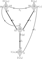
(b) A non-orientable graph

Figure 23: Orientation

Then we look at the loop lines. If every loop lines consist in the contraction of an entering and an exiting line, the graph is called orientable. Otherwise we call it non-orientable as in figure 23b.

7.2.2 Position routing

There are $n$ $\delta$ functions in an amplitude with $n$ vertices, hence $n$ linear equations for the $4n$ positions, one for each vertex. The position routing associated to the tree $T$ solves this system by passing to another equivalent system of $n$ linear equations, one for each branch of the tree. This is a triangular change of variables, of Jacobian 1. This equivalent system is obtained by summing the arguments of the $\delta$ functions of the vertices in each branch. This change of variables is exactly the $x$-space analog of the resolution of momentum conservation called momentum routing in the standard physics literature of commutative field theory, except that one should now take care of the additional $\pm$ cyclic signs.

One can prove [47] that the rank of the system of $\delta$ functions in an amplitude with $n$ vertices is

• $n-1$ if the graph is orientable

• $n$ if the graph is non-orientable

The position routing change of variables is summarized by the following lemma:

Lemma 7.2 (Position Routing).

We have, calling $I_{G}$ the remaining integrand in (7.3):

$$A_{G}= \int\Big{[}\prod_{v}\big{[}\delta(x_{v,1}-x_{v,2}+x_{v,3}-x_{v,4})\big{]}\,\Big{]}\;I_{G}(\{x_{v,i}\})$$ (7.6)

$$= \int\prod_{b}\delta\left(\sum_{l\in T_{b}\cup L_{b}}u_{l}+\sum_{l\in L_{b,+}}v_{l}-\sum_{l\in L_{b,-}}v_{l}+\sum_{f\in X_{b}}\epsilon(f)x_{f}\right)I_{G}(\{x_{v,i}\}),$$

where $\epsilon(f)$ is $\pm 1$ depending on whether the field $f$ enters or exits the branch.

We can now use the system of delta functions to eliminate variables. It is of course better to eliminate long variables as their integration costs a factor $M^{4i}$ whereas the integration of a short variable brings $M^{-4i}$. Rough power counting, neglecting all oscillations of the vertices leads therefore, in the case of an orientable graph with $N$ external fields, $n$ internal vertices and $l=2n-N/2$ internal lines at scale $i$ to:

• a factor $M^{2i(2n-N/2)}$ coming from the $M^{2i}$ factors for each line of scale $i$ in (7.5),

• a factor $M^{-4i(2n-N/2)}$ for the $l=2n-N/2$ short variables integrations,

• a factor $M^{4i(n-N/2+1)}$ for the long variables after eliminating $n-1$ of them using the delta functions.

The total factor is therefore $M^{-(N-4)i}$, the ordinary scaling of $\phi^{4}_{4}$, which means that only two and four point subgraphs ($N\leqslant 4)$ diverge when $i$ has to be summed.

In the non-orientable case, we can eliminate one additional long variable since the rank of the system of delta functions is larger by one unit! Therefore we get a power counting bound $M^{-Ni}$, which proves that only orientable graphs may diverge.

In fact we of course know that not all orientable two and four point subgraphs diverge but only the planar ones with a single external face. (It is easy to check that all such planar graphs are indeed orientable).

Since only these planar subgraphs with a single external face can be renormalized by Moyal counterterms, we need to prove that orientable, non-planar graphs or orientable planar graphs with several external faces have in fact a better power counting than this crude estimate. This can be done only by exploiting their vertices oscillations. We explain now how to do this with minimal effort.

7.2.3 Filk moves and rosettes

Following Filk [89], we can contract all lines of a spanning tree $T$ and reduce $G$ to a single vertex with “tadpole loops” called a “rosette graph”. This rosette is a cycle (which is the border of the former tree) bearing loops lines on it (see figure 24):

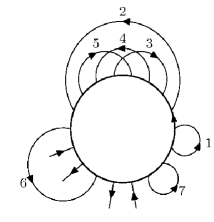
Figure 24: A rosette

Remark that the rosette can also be considered as a big vertex, with $r=2n+2$ fields, on which $N$ are external fields with external variables $x$ and $2n+2-N$ are loop fields for the corresponding $n+1-N/2$ loops. When the graph is orientable, the rosette is also orientable, which means that turning around the rosette the lines alternatively enter and exit. These lines correspond to the contraction of the fields on the border of the tree $T$ before the Filk contraction, also called the “first Filk move”.

7.2.4 Rosette factor

We start from the root and turn around the tree in the trigonometrical sense. We number separately all the fields as $1,\dots,2n+2$ and all the tree lines as $1,\dots,n-1$ in the order they are met.

Lemma 7.3.

The rosette contribution after a complete first Filk reduction is exactly:

$$\delta(v_{1}-v_{2}+\dots-v_{2n+2}+\sum_{l\in T}u_{l})e^{iVQV+iURU+iUSV}$$ (7.7)

where the $v$ variables are the long or external variables of the rosette, counted with their signs, and the quadratic oscillations for these variables is

$$VQV=\sum_{0\leqslant i<j\leqslant r}(-1)^{i+j+1}v_{i}\theta^{-1}v_{j}$$ (7.8)

We have now to analyze in detail this quadratic oscillation of the remaining long loop variables since it is essential to improve power counting. We can neglect the secondary oscillations $URU$ and $USV$ which imply short variables.

The second Filk reduction [89] further simplifies the rosette factor by erasing the loops of the rosette which do not cross any other loops or arch over external fields. It can be shown that the loops which disappear in this operation correspond to those long variables who do not appear in the quadratic form $Q$.

Using the remaining oscillating factors one can prove that non-planar graphs with genus larger than one or with more than one external face do not diverge.

The basic mechanism to improve the power counting of a single non-planar subgraph is the following:

$$\int dw_{1}dw_{2}e^{-M^{-2i_{1}}w_{1}^{2}-M^{-2i_{2}}w_{2}^{2}-iw_{1}\theta^{-1}w_{2}+w_{1}.E_{1}(x,u)+w_{2}E_{2}(x,u)}$$

$$= \int dw^{\prime}_{1}dw^{\prime}_{2}e^{-M^{-2i_{1}}(w_{1}^{\prime})^{2}-M^{-2i_{2}}(w^{\prime}_{2})^{2}+iw^{\prime}_{1}\theta^{-1}w^{\prime}_{2}+(u,x)Q(u,x)}$$

$$= KM^{4i_{1}}\int dw^{\prime}_{2}e^{-(M^{2i_{1}}+M^{-2i_{2}})(w^{\prime}_{2})^{2}}=KM^{4i_{1}}M^{-4i_{2}}\;.$$ (7.9)

In these equations we used for simplicity $M^{-2i}$ instead of the correct but more complicated factor $(\Omega/4)\tanh(\alpha/2)$ (of course this does not change the argument) and we performed a unitary linear change of variables $w^{\prime}_{1}=w_{1}+\ell_{1}(x,u)$, $w^{\prime}_{2}=w_{2}+\ell_{2}(x,u)$ to compute the oscillating $w^{\prime}_{1}$ integral. The gain in (7.2.4) is $M^{-8i_{2}}$, which is the difference between $M^{-4i_{2}}$ and the normal factor $M^{4i_{2}}$ that the $w_{2}$ integral would have cost if we had done it with the regular $e^{-M^{-2i_{2}}w_{2}^{2}}$ factor for long variables. To maximize this gain we can assume $i_{1}\leqslant i_{2}$.

This basic argument must then be generalized to each non-planar subgraph in the multiscale analysis, which is possible.

Finally it remains to consider the case of subgraphs which are planar orientable but with more than one external face. In that case there are no crossing loops in the rosette but there must be at least one loop line arching over a non trivial subset of external legs (see e.g. line $6$ in figure 24). We have then a non trivial integration over at least one external variable, called $x$, of at least one long loop variable called $w$. This “external” $x$ variable without the oscillation improvement would be integrated with a test function of scale 1 (if it is a true external line of scale $1$) or better (if it is a higher long loop variable). But we get now

$$\int dxdwe^{-M^{-2i}w^{2}-iw\theta^{-1}x+w.E_{1}(x^{\prime},u)}$$

$$= KM^{4i}\int dxe^{-M^{+2i}x^{2}}=K^{\prime}\ ,$$ (7.10)

so that a factor $M^{4i}$ in the former bound becomes ${\mathcal{O}}(1)$ hence is improved by $M^{-4i}$.

In this way we can reduce the convergence of the multiscale analysis to the problem of renormalization of planar two- and four-point subgraphs with a single external face, which we treat in the next section.

Remark that the power counting obtained in this way is still not optimal. To get the same level of precision than with the matrix base requires e.g. to display $g$ independent improvements of the type (7.2.4) for a graph of genus $g$. This is doable but basically requires a reduction of the quadratic form $Q$ for single-faced rosette (also called “hyperrosette”) into $g$ standard symplectic blocks through the so-called “third Filk move” introduced in [68]. We return to this question in section 8.2.

7.3 Renormalization

7.3.1 Four-point function

Consider the amplitude of a four-point graph $G$ which in the multiscale expansion has all its internal scales higher than its four external scales.

The idea is that one should compare its amplitude to a similar amplitude with a “Moyal factor” $\exp\Big{(}2\imath\theta^{-1}\left(x_{1}\wedge x_{2}+x_{3}\wedge x_{4}\right)\Big{)}\delta(\Delta)$ factorized in front, where $\Delta=x_{1}-x_{2}+x_{3}-x_{4}$. But precisely because the graph is planar with a single external face we understand that the external positions $x$ only couple to short variables $U$ of the internal amplitudes through the global delta function and the oscillations. Hence we can break this coupling by a systematic Taylor expansion to first order. This separates a piece proportional to “Moyal factor”, then absorbed into the effective coupling constant, and a remainder which has at least one additional small factor which gives him improved power counting.

This is done by expressing the amplitude for a graph with $N=4$, $g=0$ and $B=1$ as:

$$A(G)(x_{1},x_{2},x_{3},x_{4})= \int{\exp\Big{(}2\imath\theta^{-1}\left(x_{1}\wedge x_{2}+x_{3}\wedge x_{4}\right)\Big{)}}\prod_{\ell\in T^{i}_{k}}du_{\ell}\ C_{\ell}(u_{\ell},U_{\ell},V_{\ell})$$

$$\bigg{[}\prod_{l\in G^{i}_{k}\,\ l\not\in T}du_{l}dv_{l}C_{l}(u_{l},v_{l})\bigg{]}\ e^{\imath URU+\imath USV}$$ (7.11)

$$\Bigg{\{}{\delta(\Delta)}+\int_{0}^{1}dt\bigg{[}\mathfrak{U}\cdot\nabla\delta(\Delta+t\mathfrak{U})+\delta(\Delta+t\mathfrak{U})[\imath XQU+{\mathfrak{R}}^{\prime}(t)]\bigg{]}e^{\imath tXQU+{\mathfrak{R}}(t)}\Bigg{\}}\ .$$

where $C_{\ell}(u_{\ell},U_{\ell},V_{\ell})$ is the propagator taken at $X_{\ell}=0$, $\mathfrak{U}=\sum_{\ell}u_{\ell}$ and ${\mathfrak{R}}(t)$ is a correcting term involving $\tanh\alpha_{\ell}[X.X+X.(U+V)]$.

The first term is of the initial $\int Tr\phi\star\phi\star\phi\star\phi$ form. The rest no longer diverges, since the $U$ and ${\mathfrak{R}}$ provide the necessary small factors.

7.3.2 Two-point function

Following the same strategy we have to Taylor-expand the coupling between external variables and $U$ factors in two point planar graphs with a single external face to third order and some non-trivial symmetrization of the terms according to the two external arguments to cancel some odd contributions. The corresponding factorized relevant and marginal contributions can be then shown to give rise only to

• A mass counterterm,

• A wave function counterterm,

• An harmonic potential counterterm.

and the remainder has convergent power counting. This concludes the construction of the effective expansion in this direct space multiscale analysis.

Again the BPHZ theorem itself for the renormalized expansion follows by developing the counterterms still hidden in the effective couplings and its finiteness follows from the standard classification of forests. See however the remarks at the end of section 4.2.2.

Since the bound (7.5) works for any $\Omega\neq 0$, an additional bonus of the $x$-space method is that it proves renormalizability of the model for any $\Omega$ in $]0,1]$, whether the matrix method proved it only for $\Omega$ in $]0.5,1]$.

7.3.3 The Langmann-Szabo-Zarembo model

It is a four-dimensional theory of a Bosonic complex field defined by the action

$$S= \int\frac{1}{2}\bar{\phi}(-D^{\mu}D_{\mu}+\Omega^{2}x^{2})\phi+\lambda\bar{\phi}\star\phi\star\bar{\phi}\star\phi$$ (7.12)

where $D^{\mu}=\imath\partial_{\mu}+B_{\mu\nu}x^{\nu}$ is the covariant derivative in a magnetic field $B$.

The interaction $\bar{\phi}\star\phi\star\bar{\phi}\star\phi$ ensures that perturbation theory contains only orientable graphs. For $\Omega>0$ the $x$-space propagator still decays as in the ordinary $\phi^{4}_{4}$ case and the model has been shown renormalizable by an easy extension of the methods of the previous section [47].

However at $\Omega=0$, there is no longer any harmonic potential in addition to the covariant derivatives and the bounds are lost. We call models in this category covariant.

7.3.4 Covariant models

Consider the $x$-kernel of the operator

$$H^{-1} =\left(p^{2}+\Omega^{2}\widetilde{x}^{2}-2\imath B\left(x^{0}p_{1}-x^{1}p_{0}\right)\right)^{-1}$$ (7.13)

$$H^{-1}(x,y) =\frac{\widetilde{\Omega}}{8\pi}\int_{0}^{\infty}\frac{dt}{\sinh(2\widetilde{\Omega}t)}\,\exp\left(-\frac{\widetilde{\Omega}}{2}\frac{\cosh(2Bt)}{\sinh(2\widetilde{\Omega}t)}(x-y)^{2}\right.$$ (7.14)

$$\hskip 42.67912pt\left.-\frac{\widetilde{\Omega}}{2}{\frac{\cosh(2\widetilde{\Omega}t)-\cosh(2Bt)}{\sinh(2\widetilde{\Omega}t)}(x^{2}+y^{2})}\right.$$ (7.15)

$$\hskip 42.67912pt\left.+2\imath\widetilde{\Omega}{\frac{\sinh(2Bt)}{\sinh(2\widetilde{\Omega}t)}x\wedge y}\right)\text{\hskip 14.22636ptwith }\widetilde{\Omega}=\frac{2\Omega}{\theta}$$ (7.16)

The Gross-Neveu model or the covariant Langmann-Szabo-Zarembo models correspond to the case $B=\widetilde{\Omega}$. In these models there is no longer any confining decay for the “long variables” but only an oscillation:

$$Q^{-1}=H^{-1} =\frac{\widetilde{\Omega}}{8\pi}\int_{0}^{\infty}\frac{dt}{\sinh(2\widetilde{\Omega}t)}\,\exp\left(-\frac{\widetilde{\Omega}}{2}\coth(2\widetilde{\Omega}t)(x-y)^{2}+{2\imath\widetilde{\Omega}x\wedge y}\right)$$ (7.17)

The construction of these covariant models is more difficult, since sufficiently many oscillations must be proven independent before power counting can be established. The prototype paper which solved this problem is [51], which we briefly summarize now.

The main technical difficulty of the covariant models is the absence of decreasing functions for the long $v$ variables in the propagator replaced by an oscillation, see (7.17). Note that these decreasing functions are in principle created by integration over the $u$ variables:

$$\int du\,e^{-\frac{\widetilde{\Omega}}{2}\coth(2\widetilde{\Omega}t)u^{2}+\imath u\wedge v}= K\tanh(2\widetilde{\Omega}t)\,e^{-k\tanh(2\widetilde{\Omega}t)v^{2}}.$$ (7.18)

But to perform all these Gaussian integrations for a general graph is a difficult task (see [69]) and is in fact not necessary for a BPHZ theorem. We can instead exploit the vertices and propagators oscillations to get rational decreasing functions in some linear combinations of the long $v$ variables. The difficulty is then to prove that all these linear combinations are independent and hence allow to integrate over all the $v$ variables. To solve this problem we need the exact expression of the total oscillation in terms of the short and long variables. This consists in a generalization of the Filk’s work [89]. This has been done in [51]. Once the oscillations are proven independent, one can just use the same arguments than in the $\Phi^{4}$ case (see section 7.2) to compute an upper bound for the power counting:

Lemma 7.4 (Power counting $\text{GN}^{2}_{\Theta}$).

Let $G$ a connected orientable graph. For all $\Omega\in\left[0,1\right)$, there exists $K\in\mathbb{R}_{+}$ such that its amputated amplitude $A_{G}$ integrated over test functions is bounded by

$$\left|A_{G}\right|\leqslant K^{n}M^{-\frac{1}{2}\omega(G)}$$ (7.19)

$$\text{with }\omega(G)= \begin{cases}N-4&\text{if ($N=2$ or $N\geqslant 6$) and $g=0$,}\\ &\text{if $N=4$, $g=0$ and $B=1$,}\\ &\text{if $G$ is critical,}\\ N&\text{if $N=4$, $g=0$, $B=2$ and $G$ non-critical,}\\ N+4&\text{if $g\geqslant 1$.}\end{cases}$$ (7.20)

As in the non-commutative $\Phi^{4}$ case, only the planar graphs are divergent. But the behavior of the graphs with more than one broken face is different. Note that we already discussed such a feature in the matrix basis (see section 6.4). In the multiscale framework, the Feynman diagrams are endowed with a scale attribution which gives each line a scale index. The only subgraphs we meet in this setting have all their internal scales higher than their external ones. Then a subgraph $G$ of scale $i$ is called critical if it has $N=4,g=0,B=2$ and that the two “external” points in the second broken face are only linked by a single line of scale $j<i$. The typical example is the graph of figure 22a. In this case, the subgraph is logarithmically divergent whereas it is convergent in the $\Phi^{4}$ model. Let us now show roughly how it happens in the case of figure 22a but now in $x$-space.

The same arguments than in the $\Phi^{4}$ model prove that the integrations over the internal points of the graph 22a lead to a logarithmic divergence which means that $A_{G^{i}}\simeq{\mathcal{O}}(1)$ in the multiscale framework. But remind that there is a remaining oscillation between a long variable of this graph and the external points in the second broken face of the form $v\wedge(x-y)$. But $v$ is of order $M^{i}$ which leads to a decreasing function implementing $x-y$ of order $M^{-i}$. If these points are true external ones, they are integrated over test functions of norm $1$. Then thanks to the additional decreasing function for $x-y$ we gain a factor $M^{-2i}$ which makes the graph convergent. But if $x$ and $y$ are linked by a single line of scale $j<i$ (as in figure 22b), instead of test functions we have a propagator between $x$ and $y$. This one behaves like (see (7.17)):

$$C^{j}(x,y)\simeq M^{j}\,e^{-M^{2j}(x-y)^{2}+\imath x\wedge y}.$$ (7.21)

The integration over $x-y$ instead of giving $M^{-2j}$ gives $M^{-2i}$ thanks to the oscillation $v\wedge(x-y)$. Then we have gained a good factor $M^{-2(i-j)}$. But the oscillation in the propagator $x\wedge y$ now gives $x+y\simeq M^{2i}$ instead of $M^{2j}$ and the integration over $x+y$ cancels the preceeding gain. The critical component of figure 22a is logarithmically divergent.

This kind of argument can be repeated and refined for more general graphs to prove that this problem appears only when the external points of the auxiliary broken faces are linked only by a single lower line [51]. This phenomenon can be seen as a mixing between scales. Indeed the power counting of a given subgraph now depends on the graphs at lower scales. This was not the case in the commutative realm. Fortunately this mixing doesn’t prevent renormalization. Note that whereas the critical subgraphs are not renormalizable by a vertex-like counterterm, they are regularized by the renormalization of the two-point function at scale $j$. The proof of this point relies heavily on the fact that there is only one line of lower scale.

Let us conclude this section by mentioning the flows of the covariant models. One very interesting feature of the non-commutative $\Phi^{4}$ model is the boundedness of its flows and even the vanishing of its beta function for a special value of its bare parameters [52, 57, 58]. Note that its commutative counterpart (the usual $\phi^{4}$ model on $\mathbb{R}^{4}$) is asymptotically free in the infrared and has then an unbounded flow. It turns out that the flow of the covariant models are not regularized by the non-commutativity. The one-loop computation of the beta functions of the non-commutative Gross-Neveu model [97] shows that it is asymptotically free in the ultraviolet region as in the commutative case.

8 Parametric Representation

8.1 Ordinary Symanzik polynomials

In ordinary commutative field theory, Symanzik’s polynomials are obtained after integration over internal position variables. The amplitude of an amputated graph $G$ with external momenta $p$ is, up to a normalization, in space-time dimension $D$:

$$A_{G}(p)= \delta(\sum p)\int_{0}^{\infty}\frac{e^{-V_{G}(p,\alpha)/U_{G}(\alpha)}}{U_{G}(\alpha)^{D/2}}\prod_{l}(e^{-m^{2}\alpha_{l}}d\alpha_{l})\ .$$ (8.1)

The first and second Symanzik polynomials $U_{G}$ and $V_{G}$ are

$$U_{G}= \sum_{T}\prod_{l\not\in T}\alpha_{l}\ ,$$ (8.2a)

$$V_{G}= \sum_{T_{2}}\prod_{l\not\in T_{2}}\alpha_{l}(\sum_{i\in E(T_{2})}p_{i})^{2}\ ,$$ (8.2b)

where the first sum is over spanning trees $T$ of $G$ and the second sum is over two trees $T_{2}$, i.e. forests separating the graph in exactly two connected components $E(T_{2})$ and $F(T_{2})$; the corresponding Euclidean invariant $(\sum_{i\in E(T_{2})}p_{i})^{2}$ is, by momentum conservation, also equal to $(\sum_{i\in F(T_{2})}p_{i})^{2}$.

There are many interesting features in the parametric representation:

- It is more compact than direct or momentum space for dimension $D>2$, hence it is adapted to numerical computations.

- The dimension $D$ appears now as a simple parameter. This allows to make it non integer or even complex, at least in perturbation theory. This opens the road to the definition of dimensional regularization and renormalization, which respect the symmetries of gauge theories. This technique was the key to the first proof of the renormalizability of non-Abelian gauge theories [10].

- The form of the first and second Symanzik show an explicit positivity and democracy between trees (or two-trees): each of them appears with positive and equal coefficients.

- The locality of the counterterms is still visible (although less obvious than in direct space). It corresponds to the factorization of $U_{G}$ into $U_{S}U_{G/S}$ plus smaller terms under scaling of all the parameters of a subgraph $S$, because the leading terms are the trees whose restriction to $S$ are subtrees of $S$. One could remark that this factorization also plays a key role in the constructive RG analysis and multiscale bounds of the theory [9].

In the next two subsections we shall derive the analogs of the corresponding statements in NCVQFT. But before that let us give a brief proof of formulas (8.1). The proof of (8.2b) is similar.

Formula (8.1) is equivalent to the computation of the determinant, namely that of the quadratic form gathering the heat kernels of all the internal lines in position space, when we integrate over all vertices save one. The role of this saved vertex is crucial because otherwise the determinant of the quadratic form vanishes, i.e. the computation becomes infinite by translation invariance.

But the same determinants and problems already arose a century before Feynman graphs in the XIX century theory of electric circuits, where wires play the role of propagators and the conservation of currents at each node of the circuit play the role of conservation of momenta or translation invariance. In fact the parametric representation follows from the tree matrix theorem of Kirchoff [98], which is a key result of combinatorial theory which in its simplest form may be stated as:

Theorem 8.1 (Tree Matrix Theorem).

Let $A$ be an $n$ by $n$ matrix such that

$$\sum_{i=1}^{n}A_{ij}=0\ \ \forall j\ .$$ (8.3)

Obviously $\det A=0$. But let $A^{11}$ be the matrix $A$ with line 1 and column 1 deleted. Then

$$\det A^{11}=\sum_{T}\prod_{\ell\in T}A_{i_{\ell},j_{\ell}},$$ (8.4)

where the sum runs over all directed trees on $\{1,...,n\}$, directed away from root 1.

This theorem is a particular case of a more general result that can compute any minor of a matrix as a graphical sum over forests and more [99].

To deduce (8.1) from that theorem one defines $A_{ii}$ as the coordination of the graph at vertex $i$ and $A_{ij}$ as $-l(ij)$ where $l(ij)$ is the number of lines from vertex $i$c to vertex $j$. The line 1 and column 1 deleted correspond e.g. to fix the first vertex 1 at the origin to break translation invariance.

We include now a proof of this Theorem using Grassmann variables derived from [99], because this proof was essential for us to find the correct non commutative generalization of the parametric representation. Recall that Grasmann variables anticommute

$$\chi_{i}\chi_{j}+\chi_{j}\chi_{i}=0$$ (8.5)

hence in particular $\chi_{i}^{2}=0$, and that the Grassmann rules of integration are

$$\int d\chi=0\ ;\ \int\chi_{d}\chi=1.$$ (8.6)

Therefore we have:

Lemma 8.2.

Consider a set of $2n$ independent Grasmann variables

$${\overline{\psi}}_{1},...{\overline{\psi}}_{n},\psi_{1},...,\psi_{n}$$ (8.7)

and the integration measure

$${\rm d}{\overline{\psi}}{\rm d}\psi={\rm d}{\overline{\psi}}_{1},...{\rm d}{\overline{\psi}}_{n},{\rm d}\psi_{1},...,{\rm d}\psi_{n}$$ (8.8)

The bar is there for convenience, but it is not complex conjugation. Prove that for any matrix $A$,

$$\det A=\int{\rm d}{\overline{\psi}}{\rm d}\psi e^{-{\overline{\psi}}A\psi}\ .$$ (8.9)

More generally, if $p$ is an integer $0\leq p\leq m$, and $I=\{i_{1},\ldots,i_{p}\}$, $J=\{j_{1},\ldots,j_{p}\}$ are two ordered subsets with $p$ elements $i_{1}<\cdots<i_{p}$ and $j_{1}<\cdots<j_{p}$, if also $A^{I,J}$ denotes the $(n-p)\times(n-p)$ matrix obtained by erasing the rows of $A$ with index in $I$ and the columns of $A$ with index in $J$, then

$$\int{\rm d}{\overline{\psi}}{\rm d}\psi\ (\psi_{J}{\overline{\psi}}_{I})e^{-{\overline{\psi}}A\psi}=(-1)^{\Sigma I+\Sigma J}{\rm det}(A^{I,J})$$ (8.10)

where $(\psi_{J}{\overline{\psi}}_{I})\stackrel{{\scriptstyle\rm def}}{{=}}\psi_{j_{1}}{\overline{\psi}}_{i_{1}}\psi_{j_{2}}{\overline{\psi}}_{i_{2}}\ldots\psi_{j_{p}}{\overline{\psi}}_{i_{p}}$, $\Sigma I\stackrel{{\scriptstyle\rm def}}{{=}}i_{1}+\cdots+i_{p}$ and likewise for $\Sigma J$.

We return now to

Proof of Theorem 8.1: We use Grassmann variables to write the determinant of a matrix with one line and one raw deleted as a Grassmann integral with two corresponding sources:

$$\det A^{11}=\int({\rm d}{\overline{\psi}}{\rm d}\psi)\ (\psi_{1}{\overline{\psi}}_{1})e^{-{\overline{\psi}}A\psi}$$ (8.11)

The trick is to use (8.3) to write

$${\overline{\psi}}A\psi=\sum_{i,j=1}^{n}({\overline{\psi}}_{i}-{\overline{\psi}}_{j})A_{ij}\psi_{j}$$ (8.12)

Let, for any $j$, $1\leq j\leq n$, $B_{j}\stackrel{{\scriptstyle\rm def}}{{=}}\sum_{i=1}^{n}A_{ij}$, one then obtains by Lemma 8.2:

$$\det A^{11}=\int{\rm d}{\overline{\psi}}{\rm d}\psi\ (\psi_{1}{\overline{\psi}}_{1})\exp\left(-\sum_{i,j=1}^{n}A_{ij}({\overline{\psi}}_{i}-{\overline{\psi}}_{j})\psi_{j}\right)$$ (8.13)

$$=\int{\rm d}{\overline{\psi}}{\rm d}\psi\ (\psi_{1}{\overline{\psi}}_{1})\left[\prod_{i,j=1}^{n}\left(1-A_{ij}({\overline{\psi}}_{i}-{\overline{\psi}}_{j})\psi_{j}\right)\right]$$ (8.14)

by the Pauli exclusion principle. We now expand to get

$$\det A^{11}=\sum_{{\mathcal{G}}}\left(\prod_{\ell=(i,j)\in{\mathcal{G}}}(-A_{ij})\right)\Omega_{{\mathcal{G}}}$$ (8.15)

where ${\mathcal{G}}$ is any subset of $[n]\times[n]$, and we used the notation

$$\Omega_{{\mathcal{G}}}\stackrel{{\scriptstyle\rm def}}{{=}}\int{\rm d}{\overline{\psi}}{\rm d}\psi\ (\psi_{1}{\overline{\psi}}_{1})\left(\prod_{(i,j)\in{\mathcal{G}}}\left[({\overline{\psi}}_{i}-{\overline{\psi}}_{j})\psi_{j}\right]\right)$$ (8.16)

The theorem will now follow from the following

Lemma 8.3.

$\Omega_{{\mathcal{G}}}=0$ unless the graph ${\mathcal{G}}$ is a tree directed away from 1 in which case $\Omega_{{\mathcal{G}}}=1$.

Proof: Trivially, if $(i,i)$ belongs to ${\mathcal{G}}$, then the integrand of $\Omega_{{\mathcal{G}}}$ contains a factor ${\overline{\psi}}_{i}-{\overline{\psi}}_{i}=0$ and therefore $\Omega_{{\mathcal{G}}}$ vanishes.

But the crucial observation is that if there is a loop in ${\mathcal{G}}$ then again $\Omega_{{\mathcal{G}}}=0$. This is because then the integrand of $\Omega_{{\mathcal{F}},{\mathcal{R}}}$ contains the factor

$${\overline{\psi}}_{\tau(k)}-{\overline{\psi}}_{\tau(1)}=({\overline{\psi}}_{\tau(k)}-{\overline{\psi}}_{\tau(k-1)})+\cdots+({\overline{\psi}}_{\tau(2)}-{\overline{\psi}}_{\tau(1)})$$ (8.17)

Now, upon inserting this telescoping expansion of the factor ${\overline{\psi}}_{\tau(k)}-{\overline{\psi}}_{\tau(1)}$ into the integrand of $\Omega_{{\mathcal{F}},{\mathcal{R}}}$, the latter breaks into a sum of $(k-1)$ products. For each of these products, there exists an $\alpha\in{\mathchoice{\mathsf{ZZ}}{\mathsf{ZZ}}{\mathsf{ZZ}}{\mathsf{ZZ}}}/k{\mathchoice{\mathsf{ZZ}}{\mathsf{ZZ}}{\mathsf{ZZ}}{\mathsf{ZZ}}}$ such that the factor $({\overline{\psi}}_{\tau(\alpha)}-{\overline{\psi}}_{\tau(\alpha-1)})$ appears twice : once with the $+$ sign from the telescopic expansion of $({\overline{\psi}}_{\tau(k)}-{\overline{\psi}}_{\tau(1)})$, and once more with a $+$ (resp. $-$) sign if $(\tau(\alpha),\tau(\alpha-1))$ (resp. $(\tau(\alpha-1),\tau(\alpha))$) belongs to ${\mathcal{F}}$. Again, the Pauli exclusion principle entails that $\Omega_{{\mathcal{G}}}=0$.

Now every connected component of ${\mathcal{G}}$ must contain 1, otherwise there is no way to saturate the $d\psi_{1}$ integration.

This means that ${\mathcal{G}}$ has to be a directed tree on $\{1,...n\}$. It remains only to see now that ${\mathcal{G}}$ has to be directed away from 1, which is not too difficult.

Now Theorem 8.1 follows immediately.

8.2 Non-commutative hyperbolic polynomials, the non-covariant case

Since the Mehler kernel is still quadratic in position space it is possible to also integrate explicitly all positions to reduce Feynman amplitudes of e.g. non-commutative $\Phi^{\star 4}_{4}$ purely to parametric formulas, but of course the analogs of Symanzik polynomials are now hyperbolic polynomials which encode the richer information about ribbon graphs. These polynomials were first computed in [68] in the case of the non-covariant vulcanized $\Phi^{\star 4}_{4}$ theory. The computation relies essentially on a Grassmann variable analysis of Pfaffians which generalizes the tree matrix theorem of the previous section.

Defining the antisymmetric matrix $\sigma$ as

$$\sigma= \begin{pmatrix}\sigma_{2}&0\\ 0&\sigma_{2}\end{pmatrix}\mbox{ with}$$ (8.18)

$$\sigma_{2}= \begin{pmatrix}0&-i\\ i&0\end{pmatrix}$$ (8.19)

the $\delta-$functions appearing in the vertex contribution can be rewritten as an integral over some new variables $p_{V}$. We refer to these variables as to hypermomenta. Note that one associates such a hypermomenta $p_{V}$ to any vertex $V$ via the relation

$$\delta(x_{1}^{V}-x_{2}^{V}+x_{3}^{V}-x_{4}^{V})= \int\frac{dp^{\prime}_{V}}{(2\pi)^{4}}e^{ip^{\prime}_{V}(x_{1}^{V}-x_{2}^{V}+x_{3}^{V}-x_{4}^{V})}$$

$$= \int\frac{dp_{V}}{(2\pi)^{4}}e^{p_{V}\sigma(x_{1}^{V}-x_{2}^{V}+x_{3}^{V}-x_{4}^{V})}\ .$$ (8.20)

Consider a particular ribbon graph $G$. Specializing to dimension 4 and choosing a particular root vertex $\bar{V}$ of the graph, one can write the Feynman amplitude for $G$ in the condensed way

$${\cal A}_{G}= \int\prod_{\ell}\big{[}\frac{1-t_{\ell}^{2}}{t_{\ell}}\big{]}^{2}d\alpha_{\ell}\int dxdpe^{-\frac{\Omega}{2}XGX^{t}}$$ (8.21)

where $t_{\ell}=\tanh\frac{\alpha_{\ell}}{2}$, $X$ summarizes all positions and hypermomenta and $G$ is a certain quadratic form. If we call $x_{e}$ and $p_{\bar{V}}$ the external variables we can decompose $G$ according to an internal quadratic form $Q$, an external one $M$ and a coupling part $P$ so that

$$X= \begin{pmatrix}x_{e}&p_{\bar{V}}&u&v&p\\ \end{pmatrix}\ \ ,\ \ G=\begin{pmatrix}M&P\\ P^{t}&Q\\ \end{pmatrix}\ ,$$ (8.22)

Performing the gaussian integration over all internal variables one obtains:

$${\cal A}_{G}= \int\big{[}\frac{1-t^{2}}{t}\big{]}^{2}d\alpha\frac{1}{\sqrt{\det Q}}e^{-\frac{\widetilde{\Omega}}{2}\begin{pmatrix}x_{e}&\bar{p}\\ \end{pmatrix}[M-PQ^{-1}P^{t}]\begin{pmatrix}x_{e}\\ \bar{p}\\ \end{pmatrix}}\ .$$ (8.23)

This form allows to define the polynomials $HU_{G,\bar{v}}$ and $HV_{G,\bar{v}}$, analogs of the Symanzik polynomials $U$ and $V$ of the commutative case (see (8.1)). They are defined by

$${\cal A}_{{\bar{V}}}(\{x_{e}\},\;p_{\bar{v}})= K^{\prime}\int_{0}^{\infty}\prod_{l}[d\alpha_{l}(1-t_{l}^{2})^{2}]HU_{G,\bar{v}}(t)^{-2}e^{-\frac{HV_{G,\bar{v}}(t,x_{e},p_{\bar{v}})}{HU_{G,\bar{v}}(t)}}.$$ (8.24)

They are polynomials in the set of variables $t_{\ell}$ ($\ell=1,\ldots,L$), the hyperbolic tangent of the half-angle of the parameters $\alpha_{\ell}$.

Using now (8.23) and (8.24) the polynomial $HU_{G,\bar{v}}$ writes

$$HU_{\bar{v}}= (\det Q)^{\frac{1}{4}}\prod_{\ell=1}^{L}t_{\ell}$$ (8.25)

The main results ([68]) are

• The polynomials $HU_{G,\bar{v}}$ and $HV_{G,\bar{v}}$ have a strong positivity property. Roughly speaking they are sums of monomials with positive integer coefficients. This positive integer property comes from the fact that each such coefficient is the square of a Pfaffian with integer entries,

• Leading terms can be identified in a given “Hepp sector”, at least for orientable graphs. A Hepp sector is a complete ordering of the $t$ parameters. These leading terms which can be shown strictly positive in $HU_{G,\bar{v}}$ correspond to super-trees which are the disjoint union of a tree in the direct graph and a tree in the dual graph. Hypertrees in a graph with $n$ vertices and $F$ faces have therefore $n+F-2$ lines. (Any connected graph has hypertrees, and under reduction of the hypertree, the graph becomes a hyperrosette). Similarly one can identify “super-two-trees” $HV_{G,\bar{v}}$ which govern the leading behavior of $HV_{G,\bar{v}}$ in any Hepp sector.

From the second property, one can deduce the exact power counting of any orientable ribbon graph of the theory, just as in the matrix base.

Let us now borrow from [68] some examples of these hyperbolic polynomials. We put $s=(4\theta\Omega)^{-1}$.

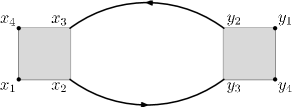
Figure 25: The bubble graph

For the bubble graph of figure 25:

$$HU_{G,v}= (1+4s^{2})(t_{1}+t_{2}+t_{1}^{2}t_{2}+t_{1}t_{2}^{2})\,,$$

$$HV_{G,v}= t_{2}^{2}\Big{[}p_{2}+2s(x_{4}-x_{1})\Big{]}^{2}+t_{1}t_{2}\Big{[}2p_{2}^{2}+(1+16s^{4})(x_{1}-x_{4})^{2}\Big{]}\,,$$

$$+t_{1}^{2}\Big{[}p_{2}+2s(x_{1}-x_{4})\Big{]}^{2}$$

For the sunshine graph fig. 26:

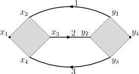
Figure 26: The Sunshine graph

$$HU_{G,v}= \Big{[}t_{1}t_{2}+t_{1}t_{3}+t_{2}t_{3}+t_{1}^{2}t_{2}t_{3}+t_{1}t_{2}^{2}t_{3}+t_{1}t_{2}t_{3}^{2}\Big{]}(1+8s^{2}+16s^{4})$$

$$+16s^{2}(t_{2}^{2}+t_{1}^{2}t_{3}^{2})\,,$$

For the non-planar sunshine graph (see fig. 27) we have:

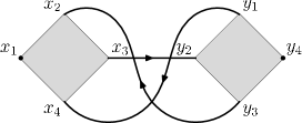
Figure 27: The non-planar sunshine graph

$$HU_{G,v}= \Big{[}t_{1}t_{2}+t_{1}t_{3}+t_{2}t_{3}+t_{1}^{2}t_{2}t_{3}+t_{1}t_{2}^{2}t_{3}+t_{1}t_{2}t_{3}^{2}\Big{]}(1+8s^{2}+16s^{4})$$

$$+4s^{2}\Big{[}1+t_{1}^{2}+t_{2}^{2}+t_{1}^{2}t_{2}^{2}+t_{3}^{2}+t_{1}^{2}t_{3}^{2}+t_{2}^{2}t_{3}^{2}+t_{1}^{2}t_{2}^{2}t_{3}^{2}\Big{]}\,,$$

We note the improvement in the genus with respect to its planar counterparts.

For the broken bubble graph (see fig. 28) we have:

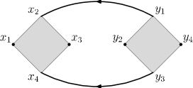
Figure 28: The broken bubble graph

$$HU_{G,v}= (1+4s^{2})(t_{1}+t_{2}+t_{1}^{2}t_{2}+t_{1}t_{2}^{2})\,,$$

$$HV_{G,v}= t_{2}^{2}\Big{[}4s^{2}(x_{1}+y_{2})^{2}+(p_{2}-2s(x_{3}+y_{4}))^{2}\Big{]}+t_{1}^{2}\Big{[}p_{2}+2s(x_{3}-y_{4})\Big{]}^{2}\,,$$

$$+t_{1}t_{2}\Big{[}8s^{2}y_{2}^{2}+2(p_{2}-2sy_{4})^{2}+(x_{1}+x_{3})^{2}+16s^{4}(x_{1}-x_{3})^{2}\Big{]}$$

$$+t_{1}^{2}t_{2}^{2}4s^{2}(x_{1}-y_{2})^{2}\,,$$

Note that $HU_{G,v}$ is identical to the one of the bubble with only one broken face. The power counting improvement comes from the broken face and can be seen only in $HV_{G,v}$.

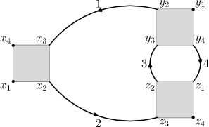
Figure 29: The half-eye graph

Finally, for the half-eye graph (see Fig. 29), we start by defining:

$$A_{24}= t_{1}t_{3}+t_{1}t_{3}t_{2}^{2}+t_{1}t_{3}t_{4}^{2}+t_{1}t_{3}t_{2}^{2}t_{4}^{2}\,.$$ (8.28)

The $HU_{G,v}$ polynomial with fixed hypermomentum corresponding to the vertex with two external legs is:

$$HU_{G,v_{1}}= (A_{24}+A_{14}+A_{23}+A_{13}+A_{12})(1+8s^{2}+16s^{4})$$

$$+t_{1}t_{2}t_{3}t_{4}(8+16s^{2}+256s^{4})+4t_{1}t_{2}t_{3}^{2}+4t_{1}t_{2}t_{4}^{2}$$

$$+16s^{2}(t_{3}^{2}+t_{2}^{2}t_{4}^{2}+t_{1}^{2}t_{4}^{2}+t_{1}^{2}t_{2}^{2}t_{3}^{2})$$

$$+64s^{4}(t_{1}t_{2}t_{3}^{2}+t_{1}t_{2}t_{4}^{2})\,,$$ (8.29)

whereas with another fixed hypermomentum we get:

$$HU_{G,v_{2}}= (A_{24}+A_{14}+A_{23}+A_{13}+A_{12})(1+8s^{2}+16s^{4})$$

$$+t_{1}t_{2}t_{3}t_{4}(4+32s^{2}+64s^{4})+32s^{2}t_{1}t_{2}t_{3}^{2}+32s^{2}t_{1}t_{2}t_{4}^{2}$$

$$+16s^{2}(t_{3}^{2}+t_{1}^{2}t_{4}^{2}+t_{2}^{2}t_{4}^{2}+t_{1}^{2}t_{2}^{3}t_{3}^{2})\,.$$ (8.30)

Note that the leading terms are identical and the choice of the root perturbs only the non-leading ones. Moreover note the presence of the $t_{3}^{2}$ term. Its presence can be understood by the fact that in the sector $t_{1},t_{2},t_{4}>t_{3}$ the subgraph formed by the lines $1,2,4$ has two broken faces. This is the sign of a power counting improvement due to the additional broken face in that sector. To exploit it, we have just to integrate over the variables of line $3$ in that sector, using the second polynomial $HV_{G^{\prime},v}$ for the triangle subgraph $G^{\prime}$ made of lines $1,2,4$.

8.3 Non-commutative hyperbolic polynomials, the covariant case

In the covariant case the diagonal coefficients on the long variables disappear but there are new antisymmetric terms proportional to $\Omega$ due to the propagator oscillations.

It is possible to reproduce easily the positivity theorem of the previous non-covariant case, because we still have sums of squares of Pfaffians. But identifying the leading terms of the polynomials under a rescaling associating to a subgraph is more difficult. It is easy to see that for transcendental values of $\Omega$, the desired leading terms cannot vanish because that would correspond to $\Omega$ being the root of a polynomial with integer coefficients. But power counting under a transcendentality condition is not very satisfying, especially because continuous RG flows also necessarily cross non transcendental points.

But thanks to a slightly more difficult analysis inspired by [95] and which involve a kind of new fourth Filk move, it is possible to prove that except again for some special cases of four point graphs with two broken faces, the power counting goes through at $\Omega<1$.

The corresponding analysis together with many examples are given in [69].

The covariant case at $\Omega=1$, also called the self-dual covariant case is very interesting, because it may be the most relevant for the study of e.g. the quantum Hall effect. Apparently it corresponds to a very degenerate non renormalizable situation because even the four point function has non logarithmic divergences as can be seen easily in the matrix basis, where the propagator is now either $1/(2m+A)$ or $1/(2n+A)$ depending on the sign of the “magnetic field” $\Omega$ . But there is a huge gauge invariance and we feel that the Ward identities of section 5 should allow renormalization of the theory even in that case.

Let us also recall that the parametric representation can be used to derive the dimensional regularization of the theory, hence perturbative quantum field theory on non-integer-dimensional Moyal space, and the associated dimensional renormalization which may be useful for renormalizing non commutative gauge theories [70].

9 Conclusion

Non-commutative QFT seemed initially to have non-renormalizable divergencies, due to UV/IR mixing. But following the Grosse-Wulkenhaar breakthrough, there has been recent rapid progress in our understanding of renormalizable QFT on Moyal spaces. We can already propose a preliminary classification of these models into different categories, according to the behavior of their propagators:

• ordinary models at $0<\Omega<1$ such as $\Phi^{\star 4}_{4}$ (which has non-orientable graphs) or $(\bar{\phi}\phi)^{2}$ models (which has none). Their propagator, roughly $(p^{2}+\Omega^{2}\tilde{x}^{2}+A)^{-1}$ is LS covariant and has good decay both in matrix space (4.11-4.14) and direct space (7.2). They have non-logarithmic mass divergencies and definitely require “vulcanization” i.e. the $\Omega$ term.

• self-dual models at $\Omega=1$ in which the propagator is LS invariant. Their propagator is even better. In the matrix base it is diagonal, e.g. of the form $G_{m,n}=(m+n+A)^{-1}$, where $A$ is a constant. The supermodels seem generically ultraviolet fixed points of the ordinary models, at which non-trivial Ward identities force the vanishing of the beta function. The flow of $\Omega$ to the $\Omega=1$ fixed point is very fast (exponentially fast in RG steps).

• covariant models such as orientable versions of LSZ or Gross-Neveu (and presumably orientable gauge theories of various kind: Yang-Mills, Chern-Simons…). They may have only logarithmic divergencies and apparently no perturbative UV/IR mixing. However the vulcanized version still appears the most generic framework for their treatment. The propagator is then roughly $(p^{2}+\Omega^{2}\tilde{x}^{2}+2\Omega\tilde{x}\wedge p)^{-1}$. In matrix space this propagator shows definitely a weaker decay (6.19) than for the ordinary models, because of the presence of a non-trivial saddle point. In direct space the propagator no longer decays with respect to the long variables, but only oscillates. Nevertheless the main lesson is that in matrix space the weaker decay can still be used; and in $x$ space the oscillations can never be completely killed by the vertices oscillations. Hence these models retain therefore essentially the power counting of the ordinary models, up to some nasty details concerning the four-point subgraphs with two external faces. Ultimately, thanks to a little conspiration in which the four-point subgraphs with two external faces are renormalized by the mass renormalization, the covariant models remain renormalizable. This is the main message of [51, 95].

• self-dual covariant models which are of the previous type but at $\Omega=1$. Their propagator in the matrix base is diagonal and depends only on one index $m$ (e.g. always the left side of the ribbon). It is of the form $G_{m,n}=(m+A)^{-1}$. In $x$ space the propagator oscillates in a way that often exactly compensates the vertices oscillations. These models have definitely worse power counting than in the ordinary case, with e.g. quadratically divergent four point-graphs (if sharp cut-offs are used). Nevertheless Ward identities can presumably still be used to show that they can still be renormalized. This probably requires a much larger conspiration to generalize the Ward identities of the supermodels.

Notice that the status of non-orientable covariant theories is not yet clarified.

Parametric representation can be derived in the non-commutative case. It implies hyperbolic generalizations of the Symanzik polynomials which condense the information about the rich topological structure of a ribbon graph. Using this representation, dimensional regularization and dimensional renormalization should extend to the non-commutative framework.

Remark that trees, which are the building blocks of the Symanzik polynomials, are also at the heart of (commutative) constructive theory, whose philosophy could be roughly summarized as “You shall use trees, but you shall not develop their loops or else you shall diverge”. It is quite natural to conjecture that hypertrees, which are the natural non-commutative objects intrinsic to a ribbon graph, should play a key combinatoric role in the yet to develop non-commutative constructive field theory.

In conclusion we have barely started to scratch the world of renormalizable QFT on non-commutative spaces. The little we see through the narrow window now open is extremely tantalizing. There exists renormalizable NCQFTs e.g. $\Phi^{\star 4}$ on ${\mathbb{R}}^{4}_{\theta}$, Gross-Neveu on ${\mathbb{R}}^{2}_{\theta}$ and they enjoy better properties than their commutative counterparts, since they have no Landau ghosts. The constructive program looks easier on non commutative geometries than on commutative ones. Non-commutative non relativistic field theories with a chemical potential seem the right formalism for a study ab initio of various problems in presence of a magnetic field, and in particular of the quantum Hall effect. The correct scaling and RG theory of this effect presumably requires to build a very singular theory (of the self-dual covariant type) because of the huge degeneracy of the Landau levels. To understand this theory and the gauge theories on non-commutative spaces seem the most obvious challenges ahead of us. An exciting possibility is that the non-commutativity of space time which killed the Landau ghost might be also a good substitute to supersymmetry by taming ultraviolet flows without requiring any new particles.

References

- [1] Neil J. Cornish, David N. Spergel, Glenn D. Starkman, and Eiichiro Komatsu, Constraining the Topology of the Universe. Phys. Rev. Lett. 92, 201302 (2004), astro-ph/0310233
- [2] V. Rivasseau and F. Vignes-Tourneret, Non-Commutative Renormalization, in Rigorous Quantum Field Theory, a Festschrift for Jacques Bros, Birkhauser Progress in Mathematics Vol. 251, 2007, hep-th/0409312, .
- [3] M. Peskin and Daniel V. Schroeder (Contributor), An Introduction to Quantum Field Theory, Perseus Publishing, (1995).
- [4] C. Itzykson and J.-B. Zuber, Quantum Field Theory, McGraw Hill, 1980.
- [5] P. Ramond, Field Theory, Addison-Wesley, 1994.
- [6] J. Glimm and A. Jaffe, Quantum Physics. A functional integral point of view. Mc Graw and Hill, New York, 1981.
- [7] Manfred Salmhofer, Renormalization: An Introduction, Texts and Monographs in Physics, Springer Verlag, 1999.
- [8] Renormalization, Poincaré Seminar 2002, in Vacuum Energy – Renormalization, Birkhäuser, Ed. by B. Duplantier and V. Rivasseau, Basel, 2003,
- [9] V. Rivasseau, From Perturbative to Constructive Renormalization, Princeton University Press, 1991.
- [10] G. ’tHooft and M. Veltman, Nucl. Phys. B50, 318 (1972).
- [11] D. Gross and F. Wilczek, Ultraviolet Behavior of Non-Abelian Gauge Theories, Phys. Rev. Lett. 30, 1343 - 1346 (1973).
- [12] H. D. Politzer, Reliable Perturbative Results for Strong Interactions? Phys. Rev. Lett. 30, 1346 - 1349 (1973).
- [13] D. Gross and F. Wilczek, Asymptotically Free Gauge Theories. I. Phys. Rev. D 8, 3633 - 3652 (1973).
- [14] K. Wilson, Renormalization group and critical phenomena, II Phase space cell analysis of critical behavior, Phys. Rev. B 4, 3184 (1974).
- [15] J. Zinn-Justin, Quantum Field Theory and Critical Phenomena, Oxford University Press, 2002.
- [16] G. Benfatto, G. Gallavotti, Renormalization Group, Princeton University Press, 1995.
- [17] G. Gentile and V. Mastropietro. Methods for the Analysis of the Lindstedt Series for KAM Tori and Renormalizability in Classical Mechanics. A Review with Some Applications. Rev. Math. Phys. 8 (1996)
- [18] W. Zimmermann, Convergence of Bogoliubov’s method for renormalization in momentum space, Comm. Math. Phys. 15, 208 (1969).
- [19] D. Kreimer, On the Hopf algebra structure of perturbative quantum field theories, Adv. Theor. Math. Phys. 2 (1998) 303–334, q-alg/9707029.
- [20] A. Connes and D. Kreimer, Renormalization in quantum field theory and the Riemann-Hilbert problem i: The hopf algebra structure of graphs and the main theorem, Commun. Math. Phys. 210 (March, 2000) 249–273.
- [21] A. Connes and D. Kreimer, Renormalization in quantum field theory and the Riemann–Hilbert problem ii: The ß-function, diffeomorphisms and the renormalization group, Commun. Math. Phys. 216 (January, 2001) 215–241.
- [22] G. Gallavotti, Perturbation Theory, in Mathematical Physics towards the XXI century, p. 275–294, ed. R. Sen, A. Gersten, Ben Gurion University Press, Ber Sheva, 1994.
- [23] J. Feldman and E. Trubowitz, Perturbation Theory for Many Fermions Systems, Helv. Phys. Acta 63, 156 (1990).
- [24] J. Feldman and E. Trubowitz, The Flow of an Electron-Phonon System to the Superconducting State, Helv. Phys. Acta 64, 213 (1991).
- [25] G. Benfatto and G. Gallavotti Perturbation theory of the Fermi surface in a quantum liquid. A general quasi-particle formalism and one dimensional systems, Journ. Stat. Physics 59, 541, 1990.
- [26] J. Feldman, J. Magnen, V. Rivasseau and E. Trubowitz, An Intrinsic 1/N Expansion for Many Fermion Systems, Europhys. Letters 24, 437 (1993).
- [27] A.B Zamolodchikov, JETP Letters 43, 1986, 731
- [28] K. Wiese, The functional renormalization group treatment of disordered systems, a review, Ann. Henri Poincaré, Vol. 4, 473 (2003).
- [29] Michael Green, John H. Schwarz and Edward Witten, Superstring theory, Cambridge University Press (1987).
- [30] A. Strominger and C. Vafa, Microscopic Origin of the Bekenstein-Hawking Entropy, Phys.Lett. B379 (1996) 99-104, hep-th/9601029
- [31] E. d’Hoker and T. Phong, Two-Loop Superstrings I, Main Formulas, Phys.Lett. B529 (2002) 241-255 hep-th/0110247
- [32] Lee Smolin, The Trouble With Physics: The Rise of String Theory, the Fall of a Science, and What Comes Next, Houghton-Mifflin, Sep. 2006.
- [33] H. S. Snyders, Quantized space-time, Phys. Rev 71, 38 (1947)
- [34] A. Connes, M. R. Douglas, and A. Schwarz, Noncommutative geometry and matrix theory: Compactification on tori, JHEP 02 (1998) 003, hep-th/9711162.
- [35] N. Seiberg and E. Witten, String theory and noncommutative geometry, JHEP 09 (1999) 032, hep-th/9908142.
- [36] M. R. Douglas and N. A. Nekrasov, Noncommutative field theory, Rev. Mod. Phys. 73 (2001) 977–1029, hep-th/0106048.
- [37] S. Minwalla, M. Van Raamsdonk, and N. Seiberg, Noncommutative perturbative dynamics, JHEP 02 (2000) 020, hep-th/9912072.
- [38] H. Grosse and R. Wulkenhaar, Power-counting theorem for non-local matrix models and renormalization, Commun. Math. Phys. 254 (2005), no. 1, 91–127, hep-th/0305066.
- [39] H. Grosse and R. Wulkenhaar, Renormalization of -theory on noncommutative in the matrix base, JHEP 12 (2003) 019, hep-th/0307017.
- [40] H. Grosse and R. Wulkenhaar, Renormalization of -theory on noncommutative in the matrix base, Commun. Math. Phys. 256 (2005), no. 2, 305–374, hep-th/0401128.
- [41] E. Langmann and R. J. Szabo, Duality in scalar field theory on noncommutative phase spaces, Phys. Lett. B533 (2002) 168–177, hep-th/0202039.
- [42] V. Rivasseau, F. Vignes-Tourneret, and R. Wulkenhaar, Renormalization of noncommutative -theory by multi-scale analysis, Commun. Math. Phys. 262 (2006) 565–594, hep-th/0501036.
- [43] E. Langmann, R. J. Szabo, and K. Zarembo, Exact solution of quantum field theory on noncommutative phase spaces, JHEP 01 (2004) 017, hep-th/0308043.
- [44] E. Langmann, R. J. Szabo, and K. Zarembo, Exact solution of noncommutative field theory in background magnetic fields, Phys. Lett. B569 (2003) 95–101, hep-th/0303082.
- [45] E. Langmann, Interacting fermions on noncommutative spaces: Exactly solvable quantum field theories in 2n+1 dimensions, Nucl. Phys. B654 (2003) 404–426, hep-th/0205287.
- [46] J. Polchinski, Renormalization and Effective Lagrangians, Nucl. Phys. B231 (1984) 269.
- [47] R. Gurau, J. Magnen, V. Rivasseau and F. Vignes-Tourneret, Renormalization of non-commutative field theory in space, Commun. Math. Phys. 267 (2006), no. 2, 515–542, hep-th/0512271.
- [48] I. Chepelev and R. Roiban, Convergence theorem for non-commutative Feynman graphs and renormalization, JHEP 03 (2001) 001, hep-th/0008090.
- [49] I. Chepelev and R. Roiban, Renormalization of quantum field theories on noncommutative . i: Scalars, JHEP 05 (2000) 037, hep-th/9911098.
- [50] R. Gurau, V. Rivasseau, and F. Vignes-Tourneret, Propagators for noncommutative field theories, Ann. H. Poincaré (2006) hep-th/0512071. Online first.
- [51] F. Vignes-Tourneret, Renormalization of the orientable non-commutative Gross-Neveu model. To appear in Ann. H. Poincaré, math-ph/0606069.
- [52] H. Grosse and R. Wulkenhaar, The beta-function in duality-covariant noncommutative -theory, Eur. Phys. J. C35 (2004) 277–282, hep-th/0402093.
- [53] K. Gawedzki and A. Kupiainen, Gross-Neveu model through convergent perturbation expansions, Comm. Math. Phys. 102, 1 (1985).
- [54] J. Feldman, J. Magnen, V. Rivasseau and R. Sénéor, A renormalizable field theory: the massive Gross-Neveu model in two dimensions, Comm. Math. Phys. 103, 67 (1986).
- [55] K. Gawedzki and A. Kupiainen, Massless theory: Rigorous control of a renormalizable asymptotically free model, Comm. Math. Phys. 99, 197 (1985).
- [56] J. Feldman, J. Magnen, V. Rivasseau and R. Sénéor, Construction of infrared by a phase space expansion, Comm. Math. Phys. 109, 437 (1987).
- [57] M. Disertori and V. Rivasseau, Two and Three Loops Beta Function of Non Commutative Theory hep-th/0610224.
- [58] M. Disertori, R. Gurau, J. Magnen and V. Rivasseau, Vanishing of Beta Function of Non Commutative to all orders, Submitted to Phys. Lett. B, hep-th/0612251.
- [59] W. Metzner and C Di Castro, “Conservation Laws and correlation functions in the Luttinger liquid,” Phys. Rev. B 47, 16107 (1993).
- [60] G. Benfatto and V. Mastropietro, “Ward Identities and Chiral Anomaly in the Luttinger Liquid,” Commun. Math. Phys. Vol. 258, 609-655 (2005).
- [61] G. Benfatto and V. Mastropietro, “Ward Identities and Vanishing of the Beta Function for d=1 Interacting Fermi Systems,” Journal of Statistical Physics, Vol. 115, 143-184 (2004)
- [62] A. Sokal, An improvement of Watson’s theorem on Borel summability, Journ. Math. Phys. 21, 261 (1980).
- [63] A. Abdesselam,A Complete Renormalization Group Trajectory Between Two Fixed Points, math-ph/0610018.
- [64] H. Grosse and H. Steinacker, Renormalization of the noncommutative model through the Kontsevich model. Nucl.Phys. B746 (2006) 202-226 hep-th/0512203.
- [65] H. Grosse and H. Steinacker, A nontrivial solvable noncommutative model in dimensions, JHEP 0608 (2006) 008 hep-th/0603052.
- [66] H. Grosse, H. Steinacker, Exact renormalization of a noncommutative model in 6 dimensions, hep-th/0607235.
- [67] Axel de Goursac, J.C. Wallet and R. Wulkenhaar, Non Commutative Induced Gauge Theory hep-th/0703075.
- [68] R. Gurau and V. Rivasseau, Parametric representation of non-commutative field theory, to appear in Commun. Math. Phys, math- ph/0606030.
- [69] V. Rivasseau and A. Tanasa, Parametric representation of “critical” noncommutative QFT models, submitted to Commun. Math. Phys., hep-th/ 0701034.
- [70] R. Gurau and A. Tanasa, work in preparation.
- [71] L. Susskind, The Quantum Hall Fluid and Non-Commutative Chern Simons Theory, hep-th/0101029
- [72] A. Polychronakos, Quantum Hall states as matrix Chern-Simons theory, JHEP 0104 (2001) 011, hep-th/0103013
- [73] S. Hellerman and M. Van Raamsdonk, Quantum Hall Physics = Noncommutative Field Theory, JHEP 0110 (2001) 039, hep-th/ 0103179
- [74] B. Duplantier, Conformal Random Geometry in Les Houches, Session LXXXIII, 2005, Mathematical Statistical Physics, A. Bovier, F. Dunlop, F. den Hollander, A. van Enter and J. Dalibard, eds., pp. 101-217, Elsevier B. V. (2006), math-ph/0608053
- [75] G. ’t Hooft, A planar diagram theory for strong interactions Nuclear Physics B, Vol. 72, p.461 (1974)
- [76] A. H. Chamseddine, A. Connes and M. Marcolli, Gravity and the standard model with neutrino mixing, arXiv:hep-th/0610241, and references therein.
- [77] V. Barger, Jing Jiang, Paul Langacker and Tianjun Li, Gauge Coupling Unification in the Standard Model, Phys.Lett. B624 (2005) 233-238, arXiv:hep-ph/0503226
- [78] V. Rivasseau, F. Vignes-Tourneret, Renormalization of non-commutative field theories, Luminy Lectures, hep-th/0702068
- [79] V. Rivasseau, An introduction to renormalization, in Poincaré Seminar 2002, ed. by B. Duplantier and V. Rivasseau. Progress in Mathematical Physics 30, Birkhäuser (2003), ISBN 3-7643-0579-7.
- [80] R. Feynman and A. Hibbs, Quantum Mechanics and Path Integrals, Mc Graw and Hill, New York 1965.
- [81] C. Itzykson and J.M Drouffe, Statistical Field Theory, Volumes 1 and 2, Cambridge University Press 1991.
- [82] Giorgio Parisi, Statistical Field Theory, Perseus Publishing 1998.
- [83] J.P. Eckmann, J. Magnen and R. Sénéor, Decay properties and Borel summability for the Schwinger functions in theories, Comm. Math. Phys. 39, 251 (1975).
- [84] J. Magnen and R. Sénéor, Phase space cell expansion and Borel summability for the Euclidean theory, Comm Math. Phys. 56, 237 (1977).
- [85] C. Kopper Renormalization Theory based on Flow Equations, in Rigorous Quantum Field Theory, a Festschrift for Jacques Bros, Birkhauser Progress in Mathenatics Vol. 251, 2007, hep-th/0508143.
- [86] M. Bergère and Y.M.P. Lam, Bogoliubov-Parasiuk theorem in the -parametric representation, Journ. Math. Phys. 17, 1546 (1976).
- [87] C. de Calan and V. Rivasseau, Local existence of the Borel transform in Euclidean , Comm. Math. Phys. 82, 69 (1981).
- [88] J. M. Gracia-Bondía and J. C. Várilly, Algebras of distributions suitable for phase space quantum mechanics. I, J. Math. Phys. 29 (1988) 869–879.
- [89] T. Filk, Divergencies in a field theory on quantum space, Phys. Lett. B376 (1996) 53–58.
- [90] V. Gayral, Heat-kernel approach to UV/IR mixing on isospectral deformation manifolds, Annales Henri Poincare 6 (2005) 991–1023, hep-th/0412233.
- [91] B. Simon, Functionnal integration and quantum physics, vol. 86 of Pure and applied mathematics. Academic Press, New York, 1979.
- [92] P. K. Mitter and P. H. Weisz, Asymptotic scale invariance in a massive Thirring model with symmetry, Phys. Rev. D8 (1973) 4410–4429.
- [93] D. J. Gross and A. Neveu, Dynamical symmetry breaking in asymptotically free field theories, Phys. Rev. D10 (1974) 3235.
- [94] C. Kopper, J. Magnen, and V. Rivasseau, Mass generation in the large N Gross-Neveu model, Commun. Math. Phys. 169 (1995) 121–180.
- [95] F. Vignes-Tourneret, Renormalization des théories de champs non commutatives. Physique théorique, Université Paris 11, september, 2006, math-ph/0612014
- [96] M. Disertori and V.Rivasseau, Continuous constructive fermionic renormalization, Annales Henri Poincaré Vol. 1 (2000) 1 hep-th/9802145.
- [97] A. Lakhoua, F. Vignes-Tourneret and J.C. Wallet, One-loop Beta Functions for the Orientable Non- commutative Gross-Neveu Model, submitted to JHEP. hep-th/0701170.
- [98] G. Kirchhoff, Über die Auflösung der Gleichungen, auf welche man bei der Untersuchung der linearen Verteilung galvanischer Ströme gefuhrt wird, Ann. Physik Chemie, 72, 497-508, (1847).
- [99] A. Abdesselam, Grassmann-Berezin Calculus and Theorems of the Matrix-Tree Type, math.CO/0306396.