Search for $D^{0}-\kern 1.99997pt\overline{\kern-1.99997ptD}{}^{0}$ Mixing Using Doubly Flavor Tagged Semileptonic Decay Modes

Abstract

We have searched for $D^{0}-\overline{D}^{0}$ mixing in $D^{*+}\rightarrow\pi^{+}D^{0}$ decays with $D^{0}\rightarrow K^{(*)}e\nu$ in a sample of $e^{+}e^{-}\rightarrow{c\overline{c}}$ events produced near 10.58 GeV. The charge of the slow pion from charged $D^{*}$ decay tags the charm flavor at production, and it is required to be consistent with the flavor of a fully reconstructed second charm decay in the same event. We observe 3 mixed candidates compared to 2.85 background events expected from simulation. We ascribe a 50% systematic uncertainty to this expected background rate. We find a central value for the mixing rate of $0.4\times 10^{-4}$. Using a frequentist method, we set corresponding 68% and 90% confidence intervals at $(-5.6,7.4)\times 10^{-4}$ and $(-13,12)\times 10^{-4}$, respectively.

I Introduction

The $D^{0}$ and $\kern 1.99997pt\overline{\kern-1.99997ptD}{}^{0}$ mesons are flavor eigenstates which are invariant in strong interactions, but are subject to electroweak interactions that permit an initial flavor eigenstate to evolve into a time-dependent mixture of $D^{0}$ and $\kern 1.99997pt\overline{\kern-1.99997ptD}{}^{0}$. In the Standard Model (SM), such oscillations proceed through both short-distance and long-distance, non-perturbative amplitudes. The expected mixing rate mediated by down-type quark box diagrams Datta and Kumbhakar (1985) and di-penguin Petrov (1997) diagrams is ${\cal O}(10^{-8}-10^{-10})$, well below the current experimental sensitivity of ${\cal O}(10^{-4}-10^{-3})$ Burdman and Shipsey (2003). The predicted range for non-perturbative, long-distance contributions Burdman and Shipsey (2003) is approximately bounded by the box diagram rate and the current experimental sensitivity. New physics predictions span the same large range Petrov (2003). While the presence of a mixing signal alone would not be a clear indication of new physics, the current experimental bounds already constrain many new physics models.

Because $D^{0}-\kern 1.99997pt\overline{\kern-1.99997ptD}{}^{0}$ mixing has been considered a potential signature for new physics, and because $C\!P$ violation in such mixing would be a signature for new physics, there have been many searches for $D^{0}-\kern 1.99997pt\overline{\kern-1.99997ptD}{}^{0}$ mixing. Typically, these searches use samples of neutral $D$ mesons produced as decay products of charged $D^{*}$ mesons where the charge of the slow pion ($\pi_{s}$) produced in association with the neutral $D$ meson tags the production flavor of the neutral $D$ meson. In semileptonic decays ($D^{0}\rightarrow K^{(*)}e\nu$), the flavor of the neutral $D$ meson when it decays is uniquely identified by the charge of the lepton. The signs of the slow pion and lepton charges are the same for unmixed decays and they differ for mixed decays. Historically, these two classes of decays are denoted as right-sign (RS) and wrong-sign (WS), respectively.

The $B$-factory experiments have searched for $D^{0}-\kern 1.99997pt\overline{\kern-1.99997ptD}{}^{0}$ mixing using semileptonic (SL) decays, where the initial flavor of the neutral $D$ meson is tagged by the charge of the slow pion from a $D^{*\pm}$ decay. The limits on $r_{\rm mix}$ (defined below) from these experiments Aubert et al. (2004); Abe et al. (2005) are listed in Table 1, along with those from recently published searches for $D^{0}-\kern 1.99997pt\overline{\kern-1.99997ptD}{}^{0}$ mixing using hadronic decay modes Asner et al. (2005); Zhang et al. (2006); Aubert et al. (2006a). In the earlier BABAR SL analysis Aubert et al. (2004), the dominant source of background in the WS signal channel originated from RS SL $D^{0}$ decays falsely associated with WS slow pion candidates. In this analysis we tag the initial flavor of the neutral $D$ meson twice: once using the slow pion from the charged $D^{*}$ decay from which the neutral $D$ decays semileptonically, and once using the flavor of a high-momentum $D$ fully reconstructed in the center-of-mass (CM) hemisphere opposite the semileptonic candidate. Tagging the flavor at production twice, rather than once, highly suppresses the background from false WS slow pions but also reduces the signal by more than an order of magnitude. The BABAR collaboration has previously used this tagging technique in a measurement of the pseudoscalar decay constant $f_{Ds}$ Aubert et al. (2006b). We have implemented additional candidate selection criteria to minimize remaining sources of background; the sensitivity of this double-tag analysis is estimated to be about the same as that of a corresponding single-tag semileptonic analysis for the same dataset.

Table 1: Limits for $r_{\rm{mix}}$ from earlier measurements in $e^{+}e^{-}$ experiments.

Experiment	Decay Mode	Integrated Luminosity		Upper Limit
BABAR  Aubert et al. (2004)	$D^{0}\rightarrow K^{(*)-}e^{+}\nu$	$87\mbox{\,fb}^{-1}$		$<42\times 10^{-4}$ (90% CL)
Belle Abe et al. (2005)	$D^{0}\rightarrow K^{(*)-}e^{+}\nu$	$254\mbox{\,fb}^{-1}$		$<10\times 10^{-4}$ (90% CL)
CLEO Asner et al. (2005)	$D^{0}\rightarrow K^{0}_{S}\pi^{-}\pi^{+}$	$9\mbox{\,fb}^{-1}$		$<63\times 10^{-4}$ (95% CL)
Belle Zhang et al. (2006)	$D^{0}\rightarrow K^{+}\pi^{-}$	$400\mbox{\,fb}^{-1}$		$<4.0\times 10^{-4}$ (95% CL)
BABAR  Aubert et al. (2006a)	$D^{0}\rightarrow K^{+}\pi^{-}\pi^{0}$	$230\mbox{\,fb}^{-1}$		$<5.4\times 10^{-4}$ (95% CL)

Charm mixing is generally characterized by two dimensionless parameters, $x\equiv\Delta m/\Gamma$ and $y\equiv\Delta\Gamma/2\Gamma$, where $\Delta m=m_{2}-m_{1}$ ($\Delta\Gamma=\Gamma_{2}-\Gamma_{1}$) is the mass (width) difference between the two neutral $D$ mass eigenstates and $\Gamma$ is the average width. If either $x$ or $y$ is non-zero, then $D^{0}$-$\kern 1.99997pt\overline{\kern-1.99997ptD}{\kern 1.00006pt}^{0}$ mixing will occur. The decay time distribution of a neutral $D$ meson which changes flavor and decays semileptonically, and thus involves no doubly interfering Cabibbo-suppressed (DCS) amplitudes, is Blaylock et al. (1995):

$$R_{\rm{mix}}(t)\cong R_{\rm{unmix}}(t)\ \frac{x^{2}+y^{2}}{4}\ \left(\frac{t}{\tau_{D^{0}}}\right)^{2},$$ (1)

where $t$ is the proper time of the $D^{0}$ decay, $\tau_{D^{0}}$ is the characteristic $D^{0}$ lifetime (= $1/\Gamma)$, $R_{\rm{unmix}}(t)\propto e^{-t/\tau_{D^{0}}}$, and the approximation is valid in the limit of small mixing rates. Sensitivity to $x$ and $y$ individually is lost with semileptonic final states. The time-integrated mixing rate $r_{\rm{mix}}$ relative to the unmixed rate is

$$r_{\rm{mix}}=\frac{x^{2}+y^{2}}{2}.$$ (2)

II The BABAR  Detector and Dataset

The data used in this analysis were collected with the BABAR detector Aubert et al. (2002) at the PEP-II storage ring. The integrated luminosity used here is approximately $344\mbox{\,fb}^{-1}$, including running both at and just below the $\mathchar 28935\relax{(4S)}$ resonance. Charged-particle momenta are measured in a tracking system consisting of a five-layer double-sided silicon vertex tracker (SVT) and a 40-layer central drift chamber (DCH), both situated in a 1.5-T axial magnetic field. An internally reflecting ring-imaging Cherenkov detector (DIRC) with fused silica bar radiators provides charged-particle identification. A CsI(Tl) electromagnetic calorimeter (EMC) is used to detect and identify photons and electrons and measure their energies. Muons are identified in the instrumented flux return system (IFR).

Electron candidates are identified by the ratio of the energy deposited in the EMC to the measured track momentum, the shower shape, the specific ionization measured in the DCH, and the Cherenkov angle measured by the DIRC. Electron identification efficiency is greater than 90% at all momenta of interest here. Pion-as-electron misidentification rates increase from about $0.05\%$ to $0.15\%$ from $500{\mathrm{\,Me\kern-1.00006ptV\!/}c}$ to 3 GeV/$c$. Kaon-as-electron misidentification rates peak at about $2.5\%$ near $500{\mathrm{\,Me\kern-1.00006ptV\!/}c}$ and decrease to $0.2\%$ above $800{\mathrm{\,Me\kern-1.00006ptV\!/}c}$.

Kaon candidates are selected using the specific ionization ($dE/dx$) measured in the DCH and SVT, and the Cherenkov angle measured in the DIRC. Kaon identification efficiency is a function of laboratory momentum; it is typically 80% or higher over the range $500{\mathrm{\,Me\kern-1.00006ptV\!/}c}$ to $3.5{\mathrm{\,Ge\kern-1.00006ptV\!/}c}$, with a maximum of about $90\%$ at $2{\mathrm{\,Ge\kern-1.00006ptV\!/}c}$. The pion-as-kaon misidentification rate is typically 1% or less for momenta below $2{\mathrm{\,Ge\kern-1.00006ptV\!/}c}$, rising to about 5% at $3.5{\mathrm{\,Ge\kern-1.00006ptV\!/}c}$.

III Analysis

The initial selection of semileptonic decay candidates follows the single-tag analysis described in Ref. Aubert et al. (2004). For each $D^{*+}\rightarrow D^{0}\pi^{+};D^{0}\rightarrow K^{(*)}e\nu$ candidate (charge conjugation is implied in all signal and tagging modes), we calculate the $D^{*+}-D^{0}$ mass difference $\Delta M=m(Ke\pi)-m(Ke)$ and the proper lifetime, as well as the output of an event selection neural network (NN). We then require that a high-momentum $D$ decaying hadronically be fully reconstructed in the opposite hemisphere of the event. This ensures that the underlying production mechanism is $e^{+}e^{-}\rightarrow c\overline{c}$ and provides a second production flavor tag. We implement additional candidate selection criteria based on studies of alternate background samples in data and a Monte Carlo (MC) simulated event sample (the “tuning” sample) to reduce various sources of background. The quark fragmentation in $e^{+}e^{-}\rightarrow c\overline{c}$ MC events is simulated using JETSET Sjostrand et al. (2001), the detector response is simulated via GEANT4 Agostinelli et al. (2003), and the resulting events are reconstructed in the same way as are real data.

To minimize bias, we use a MC sample (the “unbiased” sample) disjoint from the tuning sample, to obtain all MC based estimates of efficiencies and backgrounds. We study this sample, with effective luminosity roughly equivalent to 603 fb^-1 ($\approx 1.75\times$ data) only after all selection criteria and the full analysis method have been established. After the expected background rates are determined from the unbiased MC, we examine the signal region in the data and determine the net number of observed RS and WS signal events ($n_{\rm{RS}}$ and $n_{\rm{WS}}$). The measured mixing rate is then determined as $r_{\rm{mix}}=n_{\rm{WS}}/n_{\rm{RS}}$, corrected for the relative efficiency of the WS and RS signal selection criteria.

III.1 Reconstruction and Selection of Semileptonic Signal Candidates

Semileptonic signal candidates are selected by reconstructing the decay chain $D^{*+}\rightarrow\pi^{+}D^{0},D^{0}\rightarrow K^{(*)}e\nu$. There are no essential differences for this analysis between the $K$ and $K^{*}\rightarrow K^{\mp}\pi^{0}$ modes, either theoretically or empirically, and thus no attempt is made to reconstruct the $K^{*}$ — its charged $K$ daughter is treated as if it were a direct daughter of the $D^{0}$. Approximately 11% of signal candidates accepted in the initial selection of semileptonic canidates Aubert et al. (2004) are in the $K^{*}$ mode.

Identified $K$ and $e$ candidates of opposite charges are combined to create neutral candidate $D$ decay vertices. Only candidates with vertex fit probability $>$ 0.01 and invariant mass $<$ 1.82 GeV/$c^{2}$ are retained. This requirement is imposed to exclude all hadronic two-body $D^{0}$ decays. The average PEP-II interaction point (IP), measured on a run-to-run basis using Bhabha and $\mu^{+}\mu^{-}$ events, is taken as the production point of $D^{0}$ candidates. The $D^{0}$ decay time is measured using the transverse displacement of the $D^{0}$ vertex from the IP and the $D^{0}$ transverse momentum due to the relative narrowness of the position distribution of the IP in the transverse ($r$-$\phi$) plane Aubert et al. (2002). Neural networks are used to estimate the boost of signal candidates in the $r$-$\phi$ plane, as discussed below.

The pions from $D^{*+}$ decays are relatively soft tracks with $p^{*}_{\pi}<450$ MeV/$c$, where the asterisk denotes a parameter measured in the $e^{+}e^{-}$ CM frame. Charged tracks identified as either a charged $K$ or $e$ candidate are not considered as $\pi$ candidates. To reject poorly reconstructed tracks, $\pi$ candidates are required to have six or more SVT hits, with at least 2 hits in each of the $r$-$\phi$ and $z$ views, and at least one hit on the inner three layers in each of the $r$-$\phi$ and $z$ views. Pion candidates are refit constraining the tracks to originate from the IP, and are accepted only if the refit probability is greater than 0.01. Pion candidates meeting the above criteria are combined with $Ke$ vertex candidates to form $D^{*+}$ candidates.

A reasonable estimate of a signal candidate’s proper decay time cannot be obtained using the partial reconstruction described above and, therefore, the three orthogonal components of the $D^{0}$ CM momentum vector are estimated with three separate JetNet 3.4 Peterson et al. (1994) neural networks. Each NN has two hidden layers, and is trained and validated with a large sample $(\mathcal{O}(10^{5}))$ of simulated signal events generated separately from the other MC samples used in the analysis. The following vector inputs to the NN’s are used: ${\bf p}^{*}$($Ke$) (the momentum of the $Ke$ pair constrained by the vertex fit), ${\bf p}^{*}$($\pi$), and the event thrust vector ${\bf T^{*}}$ (calculated using all charged and neutral candidates except the $K$ and $e$ candidates). For simulated signal events, the distribution of the difference between the true ${\bf p}^{*}$($D^{0}$) direction and the NN output direction is unbiased and Gaussian with $\sigma\approx 130$ mrad. The distribution of momentum magnitude differences shows an uncertainty of $\sigma_{p}/p\approx 10\%$ for a typical signal event.

The transverse momentum of a $D^{0}$ candidate and the projections of the IP and $Ke$ vertex loci on the $r$-$\phi$ plane are used to calculate a candidate’s proper decay time. The error on the decay time, calculated using only the errors on the IP and $Ke$ vertex, is typically 0.8$\tau_{D^{0}}$, where $\tau_{D^{0}}$ is the nominal mean $D^{0}$ lifetime. The contribution of the ${\bf p}^{*}$($D^{0}$) estimator to the total decay time uncertainty is approximately $10\%$ and is ignored. Poorly reconstructed events, with calculated decay time errors greater than $2\tau_{D^{0}}$, are discarded, and only events with decay times between $-12\tau_{D^{0}}$ and $15\tau_{D^{0}}$ are retained. These criteria remove about 7% of the signal decays.

In addition to the above criteria, events are selected using a neural network trained to distinguish prompt charm signal from slow pion single-tag WS background events. The event selector NN uses a five-element input vector: $p^{*}_{Ke}$, $p^{*}_{\pi}$, $|{\bf T^{*}}|$, $\theta^{*}({\bf p}^{*}_{Ke},{\bf T^{*}})$, and $\theta^{*}({\bf p}^{*}_{K},{\bf p}^{*}_{e})$ where $\theta(\bf a,\bf b)$ denotes the opening angle between the vectors ${\bf a}$ and ${\bf b}$. It has a single hidden layer of nine nodes and is also constructed using JetNet 3.4. Figure 1(a) shows the distribution of NN output for signal candidates, RS backgrounds and WS backgrounds in double-tag unbiased MC events passing the semileptonic side event selection criteria given above. The NN output is required to be greater than 0.9 in order to yield the best statistical sensitivity to WS signal events, assuming a null mixing rate, for the double-tag dataset used here.

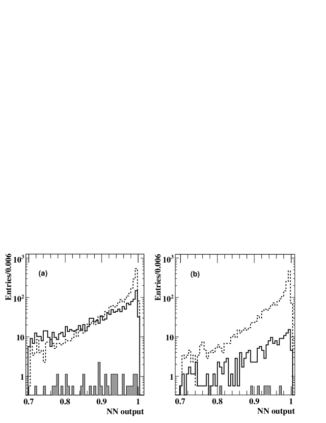
Figure 1: Event selector NN output, from double-tag luminosity-scaled unbiased MC, for events (a) passing the initial selection of semileptonic side events and (b) passing the additional semileptonic side selection criteria. The distributions shown are those for signal candidates (dashed line), RS backgrounds (solid line), and WS backgrounds (solid fill). The final event selection requires NN output $>0.9$.

III.2 The Hadronic Tagging Samples

We use the flavor of fully reconstructed charm decays in the hemisphere opposite the semileptonic signal to additionally tag the production flavor of the semileptonic signal, and thus significantly reduce the rate of wrongly tagged candidates. We use five hadronic tagging samples. Three samples explicitly require $D^{*+}$ decays: $D^{*+}\rightarrow D^{0}\pi^{+}$ where $D^{0}\rightarrow K^{-}\pi^{+}$, $D^{0}\rightarrow K^{-}\pi^{+}\pi^{0}$, and $D^{0}\rightarrow K^{-}\pi^{+}\pi^{+}\pi^{-}$; while the other two samples are not related to $D^{*+}$ decays: $D^{0}\rightarrow K^{-}\pi^{+}$ and $D^{+}\rightarrow K^{-}\pi^{+}\pi^{+}$. Candidates from the $D^{*+}$ sample are explicitly excluded from the more inclusive $D^{0}\rightarrow K^{-}\pi^{+}$ sample to ensure that the tagging samples are disjoint.

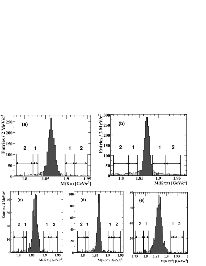
Figure 2: Invariant mass distributions of hadronic tagging candidates in data events with RS semileptonic candidates passing the initial semileptonic-side selection. The dark shaded regions denote hadronic candidates used as tags. Sideband “1” events are used to characterize “false tag” rates and sideband “2” events are used for background normalization in optimizing the hadronic mass selection. Top row: (a) $D^{0}\rightarrow K^{-}\pi^{+}$, (b) $D^{+}\rightarrow K^{-}\pi^{+}\pi^{+}$. Bottom row: $D^{*+}\rightarrow D^{0}\pi^{+}$ events in final states (c) $D^{0}\rightarrow K^{-}\pi^{+}$, (d) $D^{0}\rightarrow K^{-}\pi^{+}\pi^{+}\pi^{-}$, (e) $D^{0}\rightarrow K^{-}\pi^{+}\pi^{0}$.

The selection criteria for the tagging samples, such as the $\Delta M$ ranges for the $D^{*}$ modes or the use of production and decay vertex separation for the $D^{+}$ mode, vary from channel to channel to balance high purity against high statistics. Potential criteria are studied using candidate events from a RS sample chosen with loose requirements on the semileptonic side. To eliminate candidates from $B\kern 1.79993pt\overline{\kern-1.79993ptB}{}$ events, we require the CM momentum of the tag-side $D$ be at least $2.5{\mathrm{\,Ge\kern-1.00006ptV\!/}c}$. The individual $D^{*+}$, $D^{0}$ and $D^{+}$ tagging candidate invariant mass distributions for the final RS sample are shown in Figure 2. The purities of these tagging samples, defined as the ratio of signal in the selected mass range to the total number of candidates in that range (the darkly shaded entries in each histogram), vary from about $92\%$ for $D^{0}\rightarrow K^{-}\pi^{+}$ which do not come from $D^{*+}$ to $97.5\%$ for $D^{0}\rightarrow K^{-}\pi^{+}$ from $D^{*+}$. In the very few events where there are multiple hadronic tag candidates, we use the tag coming from the highest purity tagging sample. We reject events with multiple semileptonic signal candidates, requiring that one and only one candidate, whether RS or WS, be present after all tagging and basic semileptonic side selections are imposed. This requirement rejects approximately $13\%$ of signal candidates and a similar fraction of background candidates.

Table 2: Effects of additional semileptonic side selection criteria. Approximate cumulative acceptance rates in the double-tag unbiased MC for signal and WS background as additional selection criteria are applied, relative to acceptances following the initial semileptonic-side selection. The signal acceptances are the same for RS and WS signal samples except for the decay time cut where the entry is that for the WS sample.

Criterion	Signal Retained	WS Background Retained
$e^{\pm}$ conversion and Dalitz pair veto	100%	82%
$\pi_{s}$ $\mathrm{d}E/\mathrm{d}x$ cut	85%	66%
$\pi_{s}$ $p_{T}$ and $p_{L}$ selection	72%	36%
$m(Ke)>0.8{\mathrm{\,Ge\kern-1.00006ptV\!/}c^{2}}$	71%	30%
$(M(Ke),\Delta M)$ kinematic cut	70%	20%
600 $<t<$ 3900 fs	55%	10%

III.3 Additional Semileptonic Side Selection Criteria

Double-tagging the production flavor of the neutral $D$ mesons effectively eliminates the WS background due to real semileptonic $D$ decays paired with false slow pions from putative $D^{*+}$ decay. From studies of background events in the tuning MC sample, we find that kaon and electron candidates are almost always real kaons and electrons, respectively, with correctly assigned charges. We also find that many fake slow pion candidates are electrons produced as part of conversion pairs, or Dalitz decays of $\pi^{0}$ or, to a much lesser extent, $\eta$ mesons. These processes also contribute background tracks to the pool of electron candidates used to create $Ke$ vertices combinatorically. We consequently implement selection criteria to reject tracks which may have originated in such processes by requiring that neither an electron nor slow pion candidate form a conversion pair when combined with an oppositely charged track treated as an electron (whether identified as such or not). We further require that electron candidates not form a $\pi^{0}$ candidate when combined with a photon candidate and an oppositely charged track treated as an electron. (After applying all event selections, we find no contribution in the tuning MC sample from $\eta$ Dalitz decays.) Rejecting photon conversions and Dalitz decays reduces the total RS and WS backgrounds by about $20\%$ each, and has a negligible effect on signal efficiency.

To reduce backgrounds from kaons misidentified as electrons, we require that the laboratory momentum of electron candidates be greater than $600{\mathrm{\,Me\kern-1.00006ptV\!/}c}$. This reduces the signal efficiency by about $15\%$ and the background rate by about $35\%$. To further reduce the number of electrons that are considered as slow pions, we veto tracks where $\mathrm{d}E/\mathrm{d}x$ in the SVT is consistent with that of an electron. This reduces the signal efficiency by about $15\%$ and the background rate by about $25\%$.

We study kinematic distributions that discriminate between signal and background using data and MC events with two fully reconstructed hadronic decays of charm mesons. As a result, we require that the slow pion CM longitudinal momentum (along the axis defined by the direction opposite the tagging $D$’s CM momentum) lie in the range $150-400{\mathrm{\,Me\kern-1.00006ptV\!/}c}$ and its transverse momentum be less than $80{\mathrm{\,Me\kern-1.00006ptV\!/}c}$. This reduces the background by approximately $40\%$ and the signal efficiency by approximately $15\%$.

We require that the electron-kaon invariant mass be greater than $800{\mathrm{\,Me\kern-1.00006ptV\!/}c^{2}}$; this reduces the signal efficiency by a few percent while it reduces the background rate by approximately $20\%$. When we count the final number of signal candidates, we also require that $(M(Ke),\Delta M)$ lies inside the kinematic boundary expected for $D^{*+}\rightarrow D^{0}\pi^{+};\ D^{0}\rightarrow Ke\nu$ decays where the neutrino momentum is ignored. This has essentially no effect on signal efficiency, and reduces WS backgrounds by about $35\%$. The cumulative effects of the additional semileptonic side selection criteria are summarized in Table 2. (The selection for electron momentum $>600{\mathrm{\,Me\kern-1.00006ptV\!/}c}$ is applied prior to calculating the acceptances listed in the table.) The effects of these additional selection criteria on $D^{0}\rightarrow K^{*}e\nu$ events are reasonably consistent with those for $D^{0}\rightarrow Ke\nu$ events. The combination of the slow pion longitudinal and transverse momenta and the $(M(Ke),\Delta M)$ selections will hereinafter be referred to as the “double-tag kinematic selection”. Figure 3 shows the $\Delta M$ distributions of signal events in unbiased MC scaled to the luminosity of the data both before and after imposing the double-tag kinematic selection. The marginal efficiency resulting from applying these last selection criteria to signal events is $84\pm 1\%$.

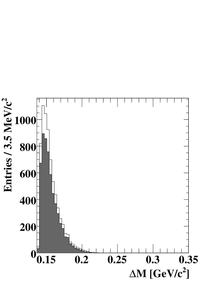
Figure 3: RS signal $\Delta M$ distribution in unbiased MC scaled to the luminosity of the data before (line) and after (solid) applying the double-tag kinematic selection.

The decay time distributions of the RS and WS signals should differ, as shown in Equation 1. The RS sample is produced with an exponential decay rate, while the WS sample should be produced with the same exponential rate modulated by $t^{2}$. Figure 4 shows the normalized lifetime distributions for reconstructed simulated RS and WS signal events passing the final tag and signal-side selection. To improve sensitivity, we select only WS candidates with measured lifetimes between 600 fs $(\approx 1.5\tau_{D^{0}})$ and 3900 fs $(\approx 9.5\tau_{D^{0}})$, which accepts approximately $80\%$ of signal and less than 30% of background. Because the RS signal-to-background ratio is comparatively very large, we accept RS candidates across the full range shown in Figure 4. This WS/RS relative efficiency has a 2% systematic uncertainty due to imperfect knowledge of the decay time resolution function. This is determined from changes in the WS/RS efficiency observed when varying the signal resolution function according to the difference between resolution functions observed in RS data and MC samples.

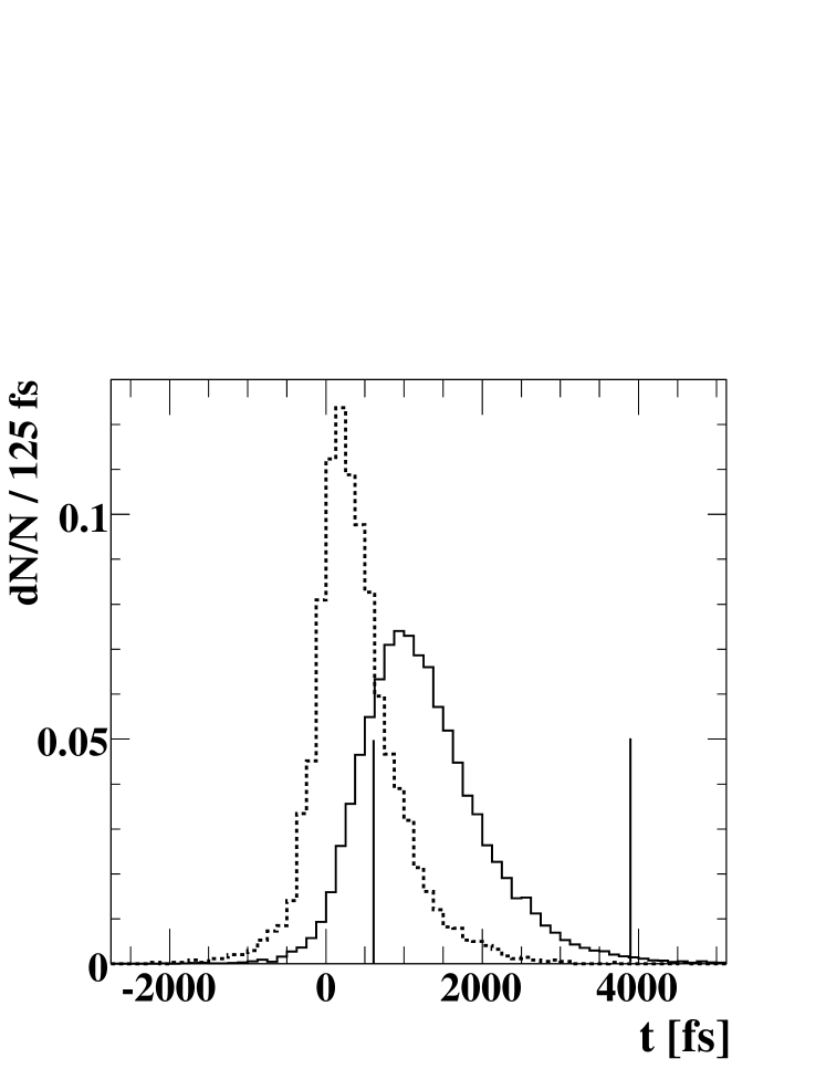
Figure 4: Normalized RS (dashed) and WS (solid) reconstructed simulated signal lifetime distributions. The solid vertical lines mark the range for the selection of the WS events.

Figure 1(b) shows the NN event selector output for RS signal, RS backgrounds and WS backgrounds in the unbiased MC sample passing the additional semileptonic side selection criteria (scaled to the luminosity of the data). The effectiveness of the additional semileptonic-side criteria in suppressing WS backgrounds while simultaneously retaining good signal efficiency can be seen by comparing Figures 1(a) and (b). Figure 5 shows the $\Delta M$ distribution of WS backgrounds passing the decay time selection in unbiased MC scaled to the luminosity of the data both before and after the double-tag kinematic selection. A total of 2.85 background candidates, the sum of the luminosity-scaled events in the solid histogram shown in the figure, is expected after all event selection criteria are applied.

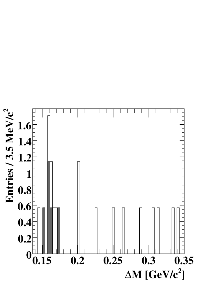
Figure 5: WS $\Delta M$ distribution for background events passing the WS decay time selection in unbiased MC scaled to the luminosity of the data before (line) and after (solid) applying the double-tag kinematic selection.

III.4 Measuring Signal Yields

To determine the mixing rate, we first determine the number of RS signal candidates by fitting the RS $\Delta M$ distribution, as described in detail below. We then estimate the expected rate of WS background events in the signal region of the data from the unbiased MC sample. Using several background control samples drawn from both data and MC, we estimate how well MC events describe real data events. Using a statistical procedure with good frequentist coverage, we combine the number of candidates observed in the WS sample, the expected background rate, and the estimated systematic uncertainty in the expected background rate to obtain a central value for the mixing rate and 68% and 90% confidence intervals. This procedure is described in detail in the appendix.

We extract the number of RS signal events from the $\Delta M$ distribution of the RS sample selected without the double-tag kinematic selection using an extended maximum likelihood fit. The likelihood function includes probability density functions (PDF’s) for the signal, the background events which peak in the signal region, and the combinatorial background. The PDF for each event class is assigned using the functional forms described in Ref. Aubert et al. (2004). The shape parameters for the combinatoric background are determined using the following technique: $D^{0}$ signal candidates in the data from one event are combined with $\pi_{s}$ candidates from another event to model the shape of this PDF. Based on MC studies, the shape of the peaking $\Delta M$ background is assumed to be the same shape as the signal. Its relative level is also determined from MC studies. The shape parameters of the signal PDF, as well as the number of RS signal events and the number of combinatorial background events, are then obtained from the likelihood fit of the data.

The main plot in Figure 6 shows the $\Delta M$ fit of the RS data before applying the double-tag kinematic selection, with the signal and background contributions overlaid. The fitted RS signal yield in this sample is $5748\pm 90$ events, with $\chi^{2}=77$ for 60 bins, where six parameters are determined from the fit. The inset plot of Figure 6 shows the RS data $\Delta M$ distribution after the double-tag kinematic selection is imposed. As noted above, the efficiency of this selection is $0.84\pm 0.01$, giving a final RS signal yield of $4780\pm 94$, which is used as the normalization in calculating the mixing rate.

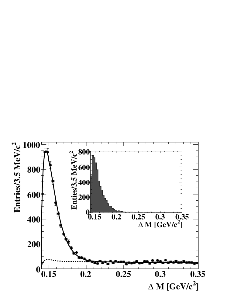
Figure 6: RS data $\Delta M$ distribution. The main plot shows the RS data (points) before imposing the double-tag kinematic selection, and the projections of the total fit PDF (solid line) and the background PDF (dashed line). The inset plot shows the RS $\Delta M$ distribution after the double-tag kinematic selection criteria are applied.

To determine the number of WS mixed events, we consider three regions of $\Delta M$: the signal region, $\Delta M\leq 0.20{\mathrm{\,Ge\kern-1.00006ptV\!/}c^{2}}$; the near background region, $0.20<\Delta M\leq 0.25{\mathrm{\,Ge\kern-1.00006ptV\!/}c^{2}}$; and the far background region, $0.25<\Delta M\leq 0.35{\mathrm{\,Ge\kern-1.00006ptV\!/}c^{2}}$. These $\Delta M$ ranges are shown in Figure  7, and are respectively labeled “1”, “2” and “3” in the plot. To avoid potential bias, we examine neither the signal region nor the near background region in the WS data sample until all of the selection criteria and the procedure for calculating confidence intervals are determined. The WS signal region may contain both signal and background events after applying the final event selection critera. As discussed above, we determine the expected number of background events from the unbiased MC sample: we observe 5 events, which scales to 2.85 for the luminosity of the data. To estimate the possible non-$c\overline{c}$ background rate, we also examine events which satisfy the semileptonic-side selection criteria but fail the tagging-side criteria because the mass of the hadronic $D$ candidate falls outside the accepted window. Since we had examined the data events in the “far” sidebands (sidebands “2”) of Figure 2 while optimizing hadronic side selection criteria, we also examine those in the “near sidebands (sidebands “1”) to estimate the number of these “false tag” events: we find no WS candidates in the near or far $\Delta M$ sideband regions in either the data or unbiased MC sample. Given the agreement between data and the unbiased MC sample, we determine the central value of the number of WS signal events by subtracting the luminosity-scaled number of unbiased MC WS background events in the signal region from the number of candidates observed in the data there.

The dark shaded entries in Figure 7 denote the $\Delta M$ distribution of WS candidates in the data after all event selection, where we observe $3$ WS candidates in the signal region and none in the sideband regions. Given the expected WS background of 2.85 events shown in the solid histogram of Figure 5, we calculate a net WS signal yield of 0.15 events. We discuss below the total error associated with the estimated number of WS background events.

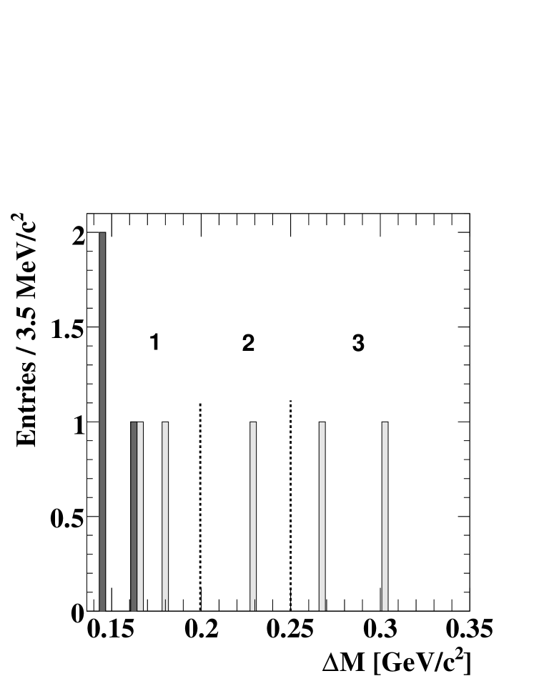
Figure 7: WS data $\Delta M$ distribution. The dark histogram shows WS events in the data passing all event selection. The light histogram shows WS events passing all selections except the double-tag kinematic selection. Region “1” is the signal region, “2” is the near sideband, and “3” is the far sideband.

III.5 Systematics and Confidence Intervals

To calculate confidence intervals for the number of mixed events observed, we first determine a systematic uncertainty associated with the WS background estimate. To do this, we compare 10 background control samples in data with the corresponding MC samples. The results of this comparison are shown in Table 3. The first line compares the number of WS events observed in the far background region of the data and the tuning MC sample. The second line compares the same numbers for the data and for the unbiased MC sample. The remaining table entries compare the number of events observed in two types of doubly-charged (DC) background samples obtained from data with those observed from the same sources in unbiased MC events. In both of the DC background samples, the kaon and the electron have the same charge sign, and are reconstructed exactly as neutral $Ke$ vertex candidates are, except for the differing charge correlation. In those additionally labeled WS, the slow pion has the same charge as the kaon, while in those additionally labeled RS, the slow pion has the opposite charge.

Table 3: Comparison of MC and data background yields. The doubly-charged (DC) MC entries refer to MC event samples disjoint from those used to optimize event selection. The “kinematic selection” refers to the double-tag kinematic selection.

Entry	Data Sample	$\Delta M$ Range (${\mathrm{\,Ge\kern-1.00006ptV\!/}c^{2}}$)	kinematic selection	Data	mm MC mm
1	WS, tuning MC	$0.25\leq\Delta M\leq 0.35$	no	$2\pm 1.4$	$2.1\pm 1.5$
2	WS, unbiased MC	$0.25\leq\Delta M\leq 0.35$	no	$2\pm 1.4$	$3.4\pm 1.4$
3	DC, RS	$\Delta M\leq 0.20$	yes	$37\pm 6$	$40\pm 5.1$
4	DC, WS	$\Delta M\leq 0.20$	yes	$36\pm 6$	$51\pm 5.8$
5	DC, RS	$\Delta M\leq 0.20$	no	$42\pm 7$	$47\pm 5.5$
6	DC, WS	$\Delta M\leq 0.20$	no	$55\pm 8$	$64\pm 6.5$
7	DC, RS	$0.20<\Delta M\leq 0.25$	no	$20\pm 5$	$24\pm 3.9$
8	DC, WS	$0.20<\Delta M\leq 0.25$	no	$13\pm 4$	$19\pm$ 3.5
9	DC, RS	$0.25\leq\Delta M\leq 0.35$	no	$20\pm 5$	$31\pm 4.5$
10	DC, WS	$0.25\leq\Delta M\leq 0.35$	no	$23\pm 5$	$18\pm 3.4$

Ignoring the correlations between entries 3,5 and 4,6 in Table 3, we estimate the consistency between the data and MC samples by calculating a summed $\chi^{2}$ for all the entries:

$$\chi^{2}(\mbox{data, MC})=\sum\limits_{i=1}^{10}\biggl{[}\frac{(x_{i}^{data}-x_{i}^{MC})^{2}}{(\sigma_{i}^{data})^{2}+(\sigma_{i}^{MC})^{2}}\biggr{]}=11.4$$ (3)

The value $\chi^{2}=11.4$ is consistent with 1 per degree of freedom. Taken together, these observations indicate that the MC estimate for the background rate in the signal region of the WS sample is reasonably accurate. We conservatively assign the largest discrepancy between the data and MC rates, 50%, as the systematic uncertainty associated with the ratio between the MC estimate of the background rate and its true value.

To determine confidence intervals for the number of WS mixed events, we adapt a suggestion made in Ref. Porter (2003). The complete statistical procedure is described in detail in the appendix; it is summarized here. We start with a likelihood function, ${\cal L}(n,n_{b};s,b)$, for the number of events observed in the signal region of the WS data sample, $n$, and the corresponding number observed in the MC sample, $n_{b}$. ${\cal L}(n,n_{b};s,b)$ depends upon the true signal rate $s$ and the true background rate $b$ in the signal region, and also accounts for the systematic uncertainty in the ratio of the true background rate in data to that estimated from MC. The value of $(s,b)$ which maximizes the likelihood function, ${{\cal L}}_{\rm max}$, is denoted by $(\hat{s},\hat{b})$. As one expects naively, $\hat{b}$ is equal to $n_{b}$ times the ratio of data and MC luminosities while $\hat{s}=n-\hat{b}$. We then search for the values of $s$ where $-{\rm ln}{\cal L}(s)$ changes by 0.50 [1.35]; here ${\cal L}(s)$ denotes the likelihood at $s$ maximized with respect to $b$. The lower and upper values of $s$ which satisfy this condition define the nominal 68% [90%] confidence interval for $s$. As discussed in the appendix, for the range of parameters relevant for this analysis, the confidence intervals produced by this procedure provide frequentist coverage which is accurate within a few percent.

III.6 Final Results and Conclusion

We observe 3 candidates for $D^{0}-\kern 1.99997pt\overline{\kern-1.99997ptD}{}^{0}$ mixing, compared to 2.85 expected background events, where we ascribe a 50% systematic uncertainty to this expected background rate. We find the central value for the number of WS signal events to be 0.15, with 68% and 90% confidence intervals $(-2.2,2.8)$ and $(-5.2,4.7)$, respectively. Accounting for the ratio of WS and RS signal efficiencies due to the cut on the measured WS decay time ($0.80\pm 0.02$), we find the central value of $r_{\rm mix}$ to be $0.4\times 10^{-4}$, with 68% and 90% confidence intervals $(-5.6,7.4)\times 10^{-4}$ and $(-13,12)\times 10^{-4}$, respectively. We ignore variations in the RS yield due to statistical error and systematic effects in the RS fit as they are negligible relative to the statistical errors associated with the WS data and MC rates as well as the 50% systematic error assigned to the ratio of MC and data WS background rates.

The sensitivity of this double-tag analysis is comparable to that expected for a single-tag analysis, see Table 1. Future analyses should be able to combine these two approaches to significantly improve overall sensitivity to charm mixing using semileptonic final states. Improved methods for reconstructing and selecting semileptonic signal candidates, the use of more hadronic tagging modes, and the additional use of semi-muonic decay modes may allow semileptonic charm mixing analyses to approach the $r_{\rm mix}$ sensitivity of analyses using hadronic final states.

IV Acknowledgments

We are grateful for the extraordinary contributions of our PEP-II colleagues in achieving the excellent luminosity and machine conditions that have made this work possible. The success of this project also relies critically on the expertise and dedication of the computing organizations that support BABAR. The collaborating institutions wish to thank SLAC for its support and the kind hospitality extended to them. This work is supported by the US Department of Energy and National Science Foundation, the Natural Sciences and Engineering Research Council (Canada), the Commissariat à l’Energie Atomique and Institut National de Physique Nucléaire et de Physique des Particules (France), the Bundesministerium für Bildung und Forschung and Deutsche Forschungsgemeinschaft (Germany), the Istituto Nazionale di Fisica Nucleare (Italy), the Foundation for Fundamental Research on Matter (The Netherlands), the Research Council of Norway, the Ministry of Science and Technology of the Russian Federation, Ministerio de Educación y Ciencia (Spain), and the Particle Physics and Astronomy Research Council (United Kingdom). Individuals have received support from the Marie-Curie IEF program (European Union) and the A. P. Sloan Foundation.

Appendix A Appendix: Statistical Method for Establishing Confidence Intervals

To estimate confidence intervals for the number of WS signal events, we adapt a method suggested in Ref. Porter (2003). For a true signal rate, $s$, and background rate, $b$, in the WS signal region, we determine probability density functions (PDF’s) for the number of background events we should observe in our Monte Carlo simulation, $n_{b}$, and the number of candidates we should observe in the WS signal region, $n$. We use these to define a global likelihood function for $s$ and $b$ which depends upon $n$ and $n_{b}$: $\mathcal{L}(s,b;n,n_{b})$. Given an observation $(n,n_{b}$), the central value for $s$ is that which maximizes $\mathcal{L}(s,b;n,n_{b})$. The boundaries of confidence intervals for $s$ are then defined by the extremum signal rates in the $(s,b)$ plane where the logarithm of the likelihood function changes by specified values based on those that would provide proper frequentist coverage in the limit of high statistics and Gaussian distributions. Assuming the PDF’s we use are correct, we validate this algorithm by checking the frequentist coverage it produces for a range of values of $s$ and $b$.

The PDF for $n_{b}$ is taken to be

$$P(n_{b};b_{\rm MC})=$$ (4)

$$N(b_{\rm MC})\int_{0}^{\infty}\frac{x^{n_{b}}}{n_{b}!}e^{-x}\frac{1}{\sigma(b_{\rm MC})}e^{-\frac{1}{2}\frac{(b_{\rm MC}-x)^{2}}{\sigma(b_{\rm MC})^{2}}}dx\,.$$

In this equation, $n_{b}$ and $b$ are as defined above; $b_{\rm MC}=\alpha b$ is the mean number of events expected in a Monte Carlo simulation with $\alpha$ times the luminosity of the data sample, and $\sigma(b_{\rm MC})=0.5\,b_{\rm MC}$ accounts for the 50% systematic uncertainty in the ratio of background rate in the data and background rate in the MC simulation. $N(b_{\rm MC})$ is the normalization such that $\sum_{n_{b}=0}^{\infty}P(n_{b};b_{\rm MC})=1$.

The PDF for the combined observation $(n,n_{b})$ is then taken to be the product of $P(n_{b};b_{\rm MC})$ and a purely Poisson term for $n$:

$$P(n;n_{b})=$$ (5)

$$P(n_{b};b_{\rm MC}=\alpha b)\times\frac{(s+b)^{n}}{n!}e^{-(s+b)}\,.$$

To obtain 90% (68%) confidence intervals, we use the following procedure.

• We write the global likelihood function for $s$ and $b$ as

  $$\mathcal{L}(s,b;n,n_{b})=$$ (6)

  $$P(n_{b};b_{\rm MC}=\alpha b)\times\frac{(s+b)^{n}}{n!}e^{-(s+b)}\,.$$

• We find the values $(\hat{s},\hat{b})$ for parameters $(s,b)$ which maximize the likelihood. These are $\hat{b}=n_{b}/a$ and $\hat{s}=n-\hat{b}$.

• With $\mathcal{L}_{max}$ the value of the likelihood at its maximum, we obtain a 90% (68%) confidence intervals for $s$, by finding the points in the $(s,b)$ plane where

  $$\Delta\rm{ln}{\cal L} \equiv \rm{ln}{\cal L}_{\rm max}-\rm{ln}{\cal L}{\it(s,b;n,n_{b})}$$

  $$= 1.35\ (0.50).$$

• We let $s_{l}$ be the minimum value of $s$ in this set and $s_{u}$ be the maximum value. The 90% (68%) confidence intervals for $s$ are the ranges $(s_{l},s_{u})$.

We have determined the frequentist coverage of this algorithm for many values of $(s,b)$ by using the PDF of Eqn. (A) to generate large samples of $(n,n_{b})$. For any one $(s,b)$, we consider the ensemble of all $(n,n_{b})$ generated. For each of these $(n,n_{b})$ we determine whether $s$ is contained in the 90% (68%) confidence interval defined using the algorithm described above. The fraction of all $(n,n_{b})$ containing the true value $s$ is called the coverage. The coverage is therefore a function of both $s$ and $b$ as well as the the level (68% or 90%). As a function of $s$ between 0 and 10, and for fixed values of $b$ between 2.5 and 7 (where 2.85 is the central value “expected” based on our observation of $n_{b}$), the coverages we calculate are close to the nominal values. In this range, the 68% intervals provide coverages between 64% and 72% with the most severe undercoverage observed for $s<2$; the 90% intervals provide coverage between 87% and 92%s with the most severe undercoverage again observed for $s<2$. The deviations from nominal coverage are relatively small. We judge the statistical properties of the quoted intervals to be sufficiently accurate for this analysis.

References

- Datta and Kumbhakar (1985) A. Datta and D. Kumbhakar, Z. Phys. C27, 515 (1985).
- Petrov (1997) A. A. Petrov, Phys. Rev. D56, 1685 (1997), eprint hep-ph/9703335.
- Burdman and Shipsey (2003) G. Burdman and I. Shipsey, Ann. Rev. Nucl. Part. Sci. 53, 431 (2003), eprint hep-ph/0310076.
- Petrov (2003) A. A. Petrov (2003), eprint hep-ph/0311371.
- Aubert et al. (2004) B. Aubert et al. (BABAR), Phys. Rev. D70, 091102 (2004), eprint hep-ex/0408066.
- Abe et al. (2005) K. Abe et al. (Belle), Phys. Rev. D72, 071101 (2005), eprint hep-ex/0507020.
- Asner et al. (2005) D. M. Asner et al. (CLEO), Phys. Rev. D72, 012001 (2005), eprint hep-ex/0503045.
- Zhang et al. (2006) L. M. Zhang et al. (BELLE), Phys. Rev. Lett. 96, 151801 (2006), eprint hep-ex/0601029.
- Aubert et al. (2006a) B. Aubert et al. (BABAR), Phys. Rev. Lett. 97, 221803 (2006a), eprint hep-ex/0608006.
- Aubert et al. (2006b) B. Aubert et al. (BABAR) (2006b), eprint hep-ex/0607094.
- Blaylock et al. (1995) G. Blaylock, A. Seiden, and Y. Nir, Phys. Lett. B355, 555 (1995), eprint hep-ph/9504306.
- Aubert et al. (2002) B. Aubert et al. (BABAR), Nucl. Instrum. Meth. A479, 1 (2002), eprint hep-ex/0105044.
- Sjostrand et al. (2001) T. Sjostrand et al., Comput. Phys. Commun. 135, 238 (2001), eprint hep-ph/0010017.
- Agostinelli et al. (2003) S. Agostinelli et al. (GEANT4), Nucl. Instrum. Meth. A506, 250 (2003).
- Peterson et al. (1994) C. Peterson, T. Rognvaldsson, and L. Lonnblad, Comput. Phys. Commun. 81, 185 (1994).
- Porter (2003) F. C. Porter (BABAR) (2003), eprint physics/0311092.