Production of a sterile species: quantum kinetics.

Abstract

Production of a sterile species is studied within an effective model of active-sterile neutrino mixing in a medium in thermal equilibrium. The quantum kinetic equations for the distribution functions and coherences are obtained from two independent methods: the effective action and the quantum master equation. The decoherence time scale for active-sterile oscillations is $\tau_{dec}=2/\Gamma_{aa}$, but the evolution of the distribution functions is determined by the two different time scales associated with the damping rates of the quasiparticle modes in the medium: $\Gamma_{1}=\Gamma_{aa}\cos^{2}\theta_{m}~{};~{}\Gamma_{2}=\Gamma_{aa}\sin^{2}\theta_{m}$ where $\Gamma_{aa}$ is the interaction rate of the active species in absence of mixing and $\theta_{m}$ the mixing angle in the medium. These two time scales are widely different away from MSW resonances and preclude the kinetic description of active-sterile production in terms of a simple rate equation. We give the complete set of quantum kinetic equations for the active and sterile populations and coherences and discuss in detail the various approximations. A generalization of the active-sterile transition probability in a medium is provided via the quantum master equation. We derive explicitly the usual quantum kinetic equations in terms of the “polarization vector” and show their equivalence to those obtained from the quantum master equation and effective action.

I Introduction

Sterile neutrinos, namely weak interaction singlets, are acquiring renewed attention as potential candidates for cold or warm dark matterdodelson ; asaka ; shi ; kev1 ; hansen ; kev2 ; kev3 ; kusenko ; kou ; dolgovrev ; pastor ; hannestad ; biermann ; michaDM , and may also be relevant in stellar collapseraffeltSN ; fuller , primordial nucleosynthesisfuller2 ; fuller3 , and as potential explanation of the anomalous velocity distributions of pulsarssegre ; fullkus ; kuse2 . Although sterile neutrinos are ubiquitous in extensions of the standard modelbook1 ; book2 ; book3 ; raffelt , the MiniBooNE collaborationminiboone has recently reported results in contradiction with those from LSNDlsnd1 ; lsnd2 that suggested a sterile neutrino with $\Delta m^{2}\sim 1~{}\textrm{eV}^{2}$ scale. Although the MiniBooNE results hint at an excess of events below $475~{}\mathrm{MeV}$ the analysis distinctly excludes two neutrino appearance-only from $\nu_{\mu}\rightarrow\nu_{e}$ oscillations with a mass scale $\Delta m^{2}\sim 1~{}\textrm{eV}^{2}$, perhaps ruling out a light sterile neutrino. However, a recent analysismalto suggests that while $(3+1)$ schemes are strongly disfavoured, $(3+2)$ neutrino schemes provide a good fit to both the LSND and MiniBooNE data, including the low energy events, because of the possibility of CP violation in these schemes, although significant tension remains.

However, sterile neutrinos as dark matter candidates would require masses in the $\mathrm{keV}$ rangedodelson ; asaka ; shi ; kev1 ; hansen ; kev2 ; kev3 ; kou ; pastor ; hannestad , hence the MiniBooNE result does not constrain a heavier variety of sterile neutrinos. The radiative decay of $\mathrm{keV}$ neutrinos would contribute to the X-ray backgroundhansen ; Xray . Analysis from the X-ray background in clusters provide constraints on the masses and mixing angles of sterile neutrinoskou ; boyarsky ; hansen2 ; kou2 , and recently it has been suggested that precision laboratory experiments on $\beta$ decay in tritium may be sensitive to $\sim\textrm{keV}$ neutrinosshapolast . Being weak interaction singlets, sterile neutrinos can only be produced via their mixing with an active species, hence any assessment of the possibility of sterile neutrinos as dark matter candidates or their role in supernovae must begin with understanding their production mechanism. Pioneering work on the description of neutrino oscillations and decoherence in a medium was cast in terms of kinetic equations for a flavor “matrix of densities”dolgov or in terms of $2\times 2$ Bloch-type equations for flavor quantum mechanical statesstodolsky ; enquist . A general field theoretical approach to neutrino mixing and kinetics was presented in sigl ; raffkin (see also raffelt ), however, while such approach in principle yields the time evolution of the distribution functions, sterile neutrino production in the early Universe is mostly studied in terms of simple phenomenological rate equationsdodelson ; kev1 ; cline ; kainu ; foot ; dibari . An early approachcline relied on a Wigner-Weisskopf effective Hamiltonian for the quantum mechanical states in the medium, while numerical studies of sterile neutrinos as possible dark matter candidateskev1 ; dibari rely on an approximate approach which inputs an effective production rate in terms of a time averaged transition probabilitykainu ; foot . More recently the sterile production rate near an MSW resonance including hadronic contributions has been studied in ref.shapo .

The rich and complex dynamics of oscillations, decoherence and damping is of fundamental and phenomenological importance not only in neutrino cosmology but also in the dynamics of meson mixing and CP violationcp ; beuthe . In ref.dolokun it was argued that the spinor nature of neutrinos is not relevant to describe the dynamics of mixing and oscillations at high energy which can then be studied within a (simpler) quantum field theory of meson degrees of freedom.

Recently we reported on a studyhobos of mixing, decoherence and relaxation in a theory of mesons which provides an accurate description of similar phenomena for mixed neutrinos. This effective theory incorporates interactions that model the medium effects associated with charge and neutral currents for neutrinos and yield a robust picture of the non-equilibrium dynamics of mixing, decoherence and equilibration which is remarkably general. The fermion nature of the distributions and Pauli blocking effects can be simply accounted for in the final resulthobos . This study implemented quantum field theory methods to obtain the non-equilibrium effective action for the “neutrino” degrees of freedom. The main ingredient in the time evolution is the full propagator for the “neutrino” degrees of freedom in the medium. The complex poles of the propagator yield the dispersion relation and damping rates of quasiparticle modes in the medium. The dispersion relations are found to be the usual ones for neutrinos in a medium with the index of refraction correction from forward scattering. For the case of two flavors, there are two damping rates which are widely different away from MSW resonances. The results of this study motivatedhozeno a deeper scrutiny of the rate equation which is often used to study sterile neutrino production in the early Universefoot ; kev1 ; dibari .

One of the observations inhozeno is that the emergence of two widely different damping time scales precludes a reliable kinetic description in terms of a time averaged transition probability suggesting that a simple rate equation to describe sterile neutrino production in the early Universe far away from MSW resonances may not be reliable.

Motivation and goals: The broad potential relevance of sterile neutrinos as warm dark matter candidates in cosmology and their impact in the late stages of stellar collapse warrant a deeper scrutiny of the quantum kinetics of production of the sterile species. Our goal is to provide a quantum field theory study of the non-equilibrium dynamics of mixing, decoherence and damping and to obtain the quantum kinetic equations that determine the production of a sterile species. We make progress towards this goal within a meson model with one active and one sterile degrees of freedom coupled to a bath of mesons in equilibrium discussed in ref.hobos . As demonstrated by the results of ref.hobos this (simpler) theory provides a remarkable effective description of propagation, mixing, decoherence and damping of neutrinos in a medium. While ref.hobos studied the approach to equilibrium focusing on the one body density matrix and single quasiparticle dynamics, in this article we obtain the non-equilibrium effective action, the quantum master equation and the complete set of quantum kinetic equations for the distribution functions and coherences. We also establish a generalization of the active-sterile transition probability based on the quantum master equation. In distinction with a recent quantum field theory treatmentshapo we seek to understand the quantum kinetics of production not only near MSW resonances, at which both time scales concidehobos ; hozeno but far away from the resonance region where the damping time scales are widely separatedhobos ; hozeno .

Similarities and differences: The scalar field model that we study has many similarities with the neutrino case but also important differences. Similarities: as demonstrated in our previous studyhobos a) the scalar model describes “flavor mixing” in a similar manner as in the case of neutrinos, where mixing arises from off-diagonal mass matrix elements, b) a medium induced “matter potential” which arises from the forward-scattering contribution to the (self) energy, c) the dispersion relation for the propagating modes is identical to those of neutrinos in a mediumnotzold ; hozeno , d) the effective mixing angles in the medium have a functional form identical to those for neutrinos in a mediumraffelt ; notzold , e) the form of the transition probability for ensemble averages in the medium is identical to that for the active-sterile neutrino transition probabilityhozeno , f) the relationship between the damping rates of the propagating modes and the active collision rate is identical to the neutrino casehozeno and g) as shown in detail in section (VI) the kinetic equations obtained are identical to those in terms of the polarization vector often quoted in the neutrino literature (see section (VI)). Differences: There are obvious differences with the neutrino case that should not be overlooked: a) spinor and chirality structure: although this is a clear difference, it is important to highlight that neither the quantum mechanical description of neutrino mixing nor the phenomenological description of neutrino kinetics account for either spinorial structure or chirality. b) Fermionic vs. Bosonic degrees of freedom, the most obvious difference is in the distribution functions, however the results obtained in sections (III-VI) for the kinetic description allow a straightforward replacement of the distribution functions for the Fermi-Dirac expressions thus automatically including Pauli blocking. c) An important difference is the matter potential, in the scalar model this is given by the one-loop Hartree self-energy, which is manifestly positive, whereas in the case of neutrinos the matter potential features a CP-odd and a CP-even contributionnotzold and it can feature either sign. The existence of an MSW resonance hinges on the sign of the self energy, in particular on the CP-odd component. However, this important difference notwithstanding, our study does not rely on or require a specific form of the matter potential, only the fact that the matter potential is diagonal in the flavor basis and in the case under consideration only the active-active matrix element is non-vanishing. Whether or not there is an MSW resonance depends on the specific form of the matter potential and in the case of neutrinos, on the CP-odd (lepton and baryon asymmetry) component of the background. Our study addresses all possible cases quite generally without the need to specify the sign (or any other quantitative aspect) of the matter potential.

Summary of results:

• i: We obtain the quantum kinetic equations for production by two different but complementary methods:

  a): the non-equilibrium effective action obtained by integrating out the “bath degrees of freedom”. This method provides a non-perturbative Dyson-like resummation of the self-energy radiative corrections and leads to the full propagators in the medium. This method makes explicit that the “neutrino” propagator in the medium along with the generalized fluctuation-dissipation relation of the bath in equilibrium are the essential ingredients for the kinetic equations and allows to identify the various approximations. It unambiguously reveals the emergence of two relaxation time scales associated with the damping rates of the propagating modes in the medium $\Gamma_{1}=\Gamma_{aa}\cos^{2}\theta_{m}~{};~{}\Gamma_{2}=\Gamma_{aa}\sin^{2}\theta_{m}$ where $\Gamma_{aa}$ is the interaction rate of the active species and $\theta_{m}$ the mixing angle in the medium, confirming the results of referenceshobos ; hozeno . These time scales determine the kinetic evolution of the distribution functions and coherences.

  b): the quantum master equation for the reduced density matrix, which is obtained by including the lowest order medium corrections to the dispersion relations (index of refraction) and mixing angles into the unperturbed Hamiltonian. This method automatically builds in the correct propagation frequencies and mixing angles in the medium.

  From the quantum master equation we obtain the kinetic equations for the distribution functions and coherences. These are identical to those obtained with the non-equilibrium effective action to leading order in perturbative quantities. After discussing the various approximations and their regime of validity we provide the full set of quantum kinetic equations for the active and sterile production as well as coherences. These are given by equations (115-120) in a form amenable to numerical implementation. We show that if the initial density matrix is off-diagonal in the basis of the propagating modes in the medium, the off-diagonal coherences are damped out in a decoherence time scale $\tau_{dec}=2/\Gamma_{aa}$. The damping of these off diagonal coherences leads to an equilibrium reduced density matrix diagonal in the basis of propagating modes in the medium.

• ii: We elucidate the nature of the various approximations that lead to the final set of quantum kinetic equations and discuss the interplay between oscillations, decoherence and damping within the realm of validity of the perturbative expansion.

• iii: We introduce a generalization of the active-sterile transition probability in the medium directly based on the quantum density matrix approach. The transition probability depends on both time scales $1/\Gamma_{1},1/\Gamma_{2}$, and the oscillatory term arising from the interference of the $1,2$ modes in the medium is damped out on the decoherence time scale $\tau_{dec}$ but this is not the relevant time scale for the build up of the populations or the transition probability far away from an MSW resonance.

• iv: We derive the quantum kinetic equation for the “polarization vector” often used in the literature directly from the kinetic equations obtained from the quantum master equation under a clearly stated approximation. We argue that the kinetic equations obtained from the quantum master equation exhibit more clearly the time scales for production and decoherence and reduce to a simple set within the regime of reliability of perturbation theory. We discuss the shortcomings of the phenomenological rate equation often used in the literature for numerical studies of sterile neutrino production.

In section (II) we introduce the model, obtain the effective action, and the full propagator from which we extract the dispersion relations and damping rates. In section (III) we define the active and sterile distribution functions and obtain their quantum kinetic non-equilibrium evolution from the effective action, discussing the various approximations. In section (IV) we obtain the quantum Master equation for the reduced density matrix, also discussing the various approximations. In this section we obtain the full set of quantum kinetic equations for the populations and coherences and show their equivalence to the results from the effective action. In section (V) we study the kinetic evolution of the off-diagonal coherences and introduce a generalization of the active-sterile transition probability in a medium directly from the quantum master equation. In section (VI) we establish the equivalence between the kinetic equations obtained from the quantum master equation and those most often used in the literature in terms of a “polarization vector”, along the way identifying the components of this “polarization vector” in terms of the populations of the propagating states in the medium $1,2$ and the coherences. While this formulation is equivalent to the quantum kinetic equations obtained from the master equation and effective action, we argue that the latter formulations yield more information, making explicit that the fundamental damping scales are the widths of the quasiparticle modes in the medium and allow to define the generalization of the transition probability in the medium. We also discuss the shortcomings of the phenomenological rate equations often invoked for numerical studies of sterile neutrino production. Section (VII) summarizes our conclusions. Two appendices elaborate on technical aspects.

II The model, effective action, and distribution functions.

We consider a model of mesons with two flavors $a,s$ in interaction with a “ vector boson” and a “flavor lepton” here denoted as $W$, $\chi_{a}$ respectively, modeling charged and neutral current interactions in the standard model. This model has been proposed as an effective description of neutrino mixing, decoherence and damping in a medium in ref.hobos to which we refer reader for details. As it will become clear below, the detailed nature of the bath fields $W,\chi_{a}$ is only relevant through their equilibrium correlation functions which can be written in dispersive form.

In terms of the field doublet

$$\Phi=\Bigg{(}\begin{array}[]{c}\phi_{a}\\ \phi_{s}\\ \end{array}\Bigg{)}$$ (1)

the Lagrangian density is

$$\mathcal{L}=\frac{1}{2}\left\{\partial_{\mu}\Phi^{T}\partial^{\mu}\Phi-\Phi^{T}\mathds{M}^{2}\Phi\right\}+\mathcal{L}_{0}[W,\chi]+G\,W\,\phi_{a}\chi_{a}+G\phi^{2}_{a}\chi^{2}_{a}$$ (2)

where the mass matrix is given by

$$\mathds{M}^{2}=\left(\begin{array}[]{cc}M^{2}_{aa}&M^{2}_{as}\\ M^{2}_{as}&M^{2}_{ss}\\ \end{array}\right)$$ (3)

and $\mathcal{L}_{0}[W,\chi]$ is the free field Lagrangian density for $W,\chi$ which need not be specified.

The mesons $\phi_{a,s}$ play the role of the active and sterile flavor neutrinos, $\chi_{a}$ the role of the charged lepton associated with the active flavor and $W$ a charged current, for example the proton-neutron current $\overline{p}\gamma^{\mu}(1-g_{A}\gamma_{5})n$ or a similar quark current. The coupling $G$ plays the role of $G_{F}$. The interaction between the “neutrino” doublet and the $W,\chi_{a}$ fields is of the same form as that studied in ref.raffelt ; sigl ; raffkin for neutral and charged current interactions.

The last term in the Lagrangian density (2) allows to model the matter effective potential from forward scattering in the medium by replacing $\chi^{2}_{a}$ by its expectation value in the statistical ensemble, $\langle\chi^{2}_{a}\rangle$. The resulting term $G\phi^{2}_{a}\langle\chi^{2}_{a}\rangle$ effectively models a matter potential from forward scattering in the mediumraffelt . While in the bosonic case $\langle\chi^{2}_{a}\rangle$ is manifestly positive, in the fermionic case the effective potential from forward scattering in the medium features two distinct contributionsnotzold : a CP odd contribution which is proportional to the lepton and baryon asymmetries, and a CP even contribution that only depends on the temperature. However, as it will become clear below, we do not need to specify the precise form of the matter potential or of the bath degrees of freedom, only the fact that the matter potential is diagonal in the flavor basis with only entry in the $a-a$ component, and the spectral properties of the correlation function of bath degrees of freedom are necessary.

The flavor $\phi_{a,s}$ and the mass basis fields $\varphi_{1,2}$ are related by an orthogonal transformation $\Phi=U(\theta)\,\varphi$

$$\left(\begin{array}[]{c}\phi_{a}\\ \phi_{s}\\ \end{array}\right)=U(\theta)~{}\Bigg{(}\begin{array}[]{c}\varphi_{1}\\ \varphi_{2}\\ \end{array}\Bigg{)}~{}~{};~{}~{}U(\theta)=\Bigg{(}\begin{array}[]{cc}\cos\theta&\sin\theta\\ -\sin\theta&\cos\theta\\ \end{array}\Bigg{)}$$ (4)

where the orthogonal matrix $U(\theta)$ diagonalizes the mass matrix $\mathds{M}^{2}$, namely

$$U^{-1}(\theta)\,\mathds{M}^{2}\,U(\theta)=\Bigg{(}\begin{array}[]{cc}M^{2}_{1}&0\\ 0&M^{2}_{2}\\ \end{array}\Bigg{)}$$ (5)

In the flavor basis the mass matrix $\mathbb{M}$ can be written in terms of the vacuum mixing angle $\theta$ and the eigenvalues of the mass matrix as

$$\mathds{M}^{2}=\overline{M}^{\,2}\,\mathds{1}+\frac{\delta M^{2}}{2}\left(\begin{array}[]{cc}-\cos 2\theta&\sin 2\theta\\ \sin 2\theta&\cos 2\theta\\ \end{array}\right)$$ (6)

where we introduced

$$\overline{M}^{\,2}=\frac{1}{2}(M^{2}_{1}+M^{2}_{2})~{}~{};~{}~{}\delta M^{2}=M^{2}_{2}-M^{2}_{1}\,.$$ (7)

For the situation under consideration with keV sterile neutrinos with small vacuum mixing angle $\theta\ll 1$

$$M_{aa}\sim M_{1}~{};~{}M_{ss}\sim M_{2}$$ (8)

and in the vacuum

$$\phi_{a}\sim\phi_{1}~{};~{}\phi_{s}\sim\phi_{2}\,.$$ (9)

We focus on the description of the dynamics of the “system fields” $\phi_{\alpha},~{}\alpha=a,s$. The strategy is to consider the time evolved full density matrix and trace over the bath degrees of freedom $\chi,W$. It is convenient to write the Lagrangian density (2) as

$${\cal L}[\phi_{\alpha},\chi_{\alpha},W]={\cal L}_{0}[\phi]+{\cal L}_{0}[W,\chi]+G\phi_{a}\mathcal{O}_{a}+G\phi^{2}_{a}\chi^{2}_{a}$$ (10)

where

$$\mathcal{O}_{a}=\chi_{a}\,W\,.$$ (11)

and ${\mathcal{L}}_{0}[\cdots]$ are the free Lagrangian densities for the fields $\phi_{\alpha},\chi_{a},W$ respectively. The fields $\phi_{\alpha}$ are considered as the “system” and the fields $\chi_{a},W$ are treated as a bath in thermal equilibrium at a temperature $T\equiv 1/\beta$. We consider a factorized initial density matrix at a time $t_{0}=0$ of the form

$$\widehat{\rho}(0)={\rho}_{\Phi}(0)\otimes\rho_{B}(0)~{}~{};~{}~{}\rho_{B}(0)=e^{-\beta\,H_{0}[\chi,W]}$$ (12)

where $H_{0}[\chi,W]$ is Hamiltonian for the fields $\chi_{a},W$ in absence of interactions with the neutrino field $\phi_{a}$.

Although this factorized form of the initial density matrix leads to initial transient dynamics, we are interested in the long time dynamics, in particular in the long time limit.

The bath fields $\chi_{\alpha},W$ will be “integrated out” yielding a reduced density matrix for the fields $\phi_{\alpha}$ in terms of an effective real-time functional, known as the influence functionalfeyver in the theory of quantum brownian motion. The reduced density matrix can be represented by a path integral in terms of the non-equilibrium effective action that includes the influence functional. This method has been used extensively to study quantum brownian motionfeyver ; leggett , and quantum kineticsboyalamo ; hoboydavey and more recently in the study of the non-equilibrium dynamics of thermalization in a similar modelhobos . The time evolution of the initial density matrix is given by

$$\widehat{\rho}(t)=e^{-iH(t-t_{0})}\widehat{\rho}(t_{0})e^{iH(t-t_{0})}$$ (13)

Where the total Hamiltonian $H$ is

$$H=H_{0}[\phi]+H_{0}[\chi,W]+H_{I}[\phi,\chi,W]$$ (14)

Denoting all the fields collectively as $X$ to simplify notation, the density matrix elements in the field basis are given by

$$\langle X|\widehat{\rho}(t)|X^{\prime}\rangle=\int DX_{i}DX^{\prime}_{i}~{}\langle X|e^{-iH(t-t_{0})}|X_{i}\rangle~{}\langle X_{i}|\widehat{\rho}(t_{0})|X^{\prime}_{i}\rangle~{}\langle X^{\prime}_{i}|e^{iH(t-t_{0})}|X^{\prime}\rangle\,.$$ (15)

The density matrix elements in the field basis can be expressed as a path integral by using the representations

$$\langle X|e^{-iH(t-t_{0})}|X_{i}\rangle=\int\mathcal{D}X^{+}~{}e^{i\int_{t_{0}}^{t}dt\int d^{3}x\mathcal{L}[X^{+}]}~{}~{};~{}~{}X^{+}(t_{0})=X_{i};X^{+}(t)=X\,.$$ (16)

Similarly

$$\langle X^{\prime}_{i}|e^{iH(t-t_{0})}|X^{\prime}\rangle=\int\mathcal{D}X^{-}~{}e^{-i\int_{t_{0}}^{t}dt\int d^{3}x\mathcal{L}[X^{-}]}~{}~{};~{}~{}X^{-}(t_{0})=X^{\prime}_{i};X^{-}(t)=X^{\prime}\,.$$ (17)

Therefore the full time evolution of the density matrix can be systematically studied via the path integral

$$\mathcal{Z}=\int\mathcal{D}X^{+}\mathcal{D}X^{-}e^{i\int_{t_{0}}^{t}dt\int d^{3}x\left\{\mathcal{L}[X^{+}]-\mathcal{L}[X^{-}]\right\}}\,,$$ (18)

with the boundary conditions discussed above. This representation allows to obtain expectation values or correlation functions $\mathcal{C}(X,X_{i},X^{\prime}_{i},X^{\prime};t,t^{\prime})$ which depend on the values of the fields $X_{i};X^{\prime}_{i}$ through the initial conditions. In order to obtain expectation values or correlation functions in the full time evolved density matrix, the results from the path integral must be averaged in the initial density matrix $\widehat{\rho}(t_{0})$, namely

$$\langle\mathcal{C}(X,X^{\prime};t,t^{\prime})\rangle\equiv\int DX_{i}DX^{\prime}_{i}~{}\langle X_{i}|\widehat{\rho}(t_{0})|X^{\prime}_{i}\rangle~{}\mathcal{C}(X,X_{i},X^{\prime}_{i},X^{\prime};t,t^{\prime})\,.$$ (19)

We will only study correlation functions of the “system” fields $\phi_{\alpha}$, therefore we carry out the trace over the $\chi_{a}$ and $W$ degrees of freedom in the path integral (18) systematically in a perturbative expansion in $G$. The resulting series is re-exponentiated to yield the non-equilibrium effective action and the generating functional of connected correlation functions of the fields $\phi_{\alpha}$. This procedure has been explained in detail in referencesboyalamo ; hoboydavey and more recently in hobos within a model similar to the one under consideration. Following the procedure detailed in these references we obtain the non-equilibrium effective action up to order $G^{2}$ and quadratic in the fields $\phi_{\alpha}$ neglecting higher order non-linearities,

$$iL_{eff}[\phi^{+},\phi^{-}] = \sum_{\vec{k}}\Bigg{\{}\frac{i}{2}\int dt\Big{[}\dot{\phi}^{+}_{\alpha,\vec{k}}(t)\dot{\phi}^{+}_{\alpha,-\vec{k}}(t)-\phi^{+}_{\alpha,\vec{k}}(t)(k^{2}\mathds{1}+\mathds{M}^{2}+\mathds{V})\phi^{+}_{\beta,-\vec{k}}(t)$$ (20)

$$-\dot{\phi}^{-}_{\alpha,\vec{k}}(t)\dot{\phi}^{-}_{\alpha,-\vec{k}}(t)+\phi^{-}_{\alpha,\vec{k}}(t)(k^{2}\,\mathds{1}+\mathds{M}^{2}+\mathds{V})\phi^{-}_{-\vec{k}}(t)\Big{]}$$

$$-\frac{G^{2}}{2}\int dt\int dt^{\prime}\left[\phi^{+}_{a,\vec{k}}(t){\cal G}^{++}(k;t,t^{\prime})\phi^{+}_{a,-\vec{k}}(t^{\prime})+\phi^{-}_{a,\vec{k}}(t){\cal G}^{--}(k;t,t^{\prime})\phi^{-}_{a,-\vec{k}}(t^{\prime})\right.$$

$$\left.-\phi^{+}_{a,\vec{k}}(t){\cal G}^{+-}(k;t,t^{\prime})\phi^{-}_{a,-\vec{k}}(t^{\prime})-\phi^{-}_{a,\vec{k}}(t){\cal G}^{-+}(k;t,t^{\prime})\phi^{+}_{a,-\vec{k}}(t^{\prime})\right]\Bigg{\}}$$

where the matter potential is

$$\mathds{V}=\left(\begin{array}[]{cc}V_{aa}&0\\ 0&0\\ \end{array}\right)~{}~{};~{}~{}V_{aa}=G\langle\chi^{2}_{a}\rangle\,,$$ (21)

with the average in the initial bath density matrix. In the bosonic model, the corresponding one-loop diagram at order $G$ that yields the matter potential and effectively models forward scattering in the medium is depicted in figure (1).

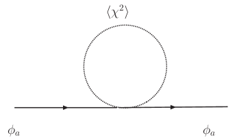
Figure 1: One loop self-energy for the active species at order $G$, corresponding to the matter potential $V_{aa}=G\langle\chi^{2}\rangle$.

In the fermionic theory, the matter potential in a medium at finite temperature and density has two distinct contributionsnotzold : a CP-odd term proportional to the lepton and baryon asymmetries and a CP-even term that only depends on the temperature. The sign of these contributions may be either positive or negative depending on which term dominatesnotzold . The presence of an MSW resonance in the medium depends crucially on the CP-odd contribution. In the case of sterile neutrinos with masses in the $keV$ range, only for non-vanishing lepton asymmetry is there an MSW resonance. However, the only important point for the analysis that follows is that the matter potential is diagonal in the flavor basis, with only entry $V_{aa}$, namely the form of the matrix given by eqn. (21), but of course the matrix element $V_{aa}$ itself will be different for fermions.

The correlation functions $\mathcal{G}(t,t^{\prime})\sim\langle\mathcal{O}_{a}(t)\mathcal{O}_{a}(t^{\prime})\rangle=\langle W(t)W(t^{\prime})\rangle\,\langle\chi_{a}(t)\chi_{a}(t^{\prime})\rangle$ are also determined by averages in the initial equilibrium bath density matrix and their explicit form is given in referencehobos (see also appendix (B)).

Performing the trace over the bath degrees of freedom the resulting non-equilibrium effective action acquires a simpler form in terms of the Wigner center of mass and relative variableshobos ; boyalamo ; hoboydavey

$$\Psi_{\alpha}(\vec{x},t)=\frac{1}{2}\left(\phi^{+}_{\alpha}(\vec{x},t)+\phi^{-}_{\alpha}(\vec{x},t)\right)\;\;;\;\;R_{\alpha}(\vec{x},t)=\left(\phi^{+}_{\alpha}(\vec{x},t)-\phi^{-}_{\alpha}(\vec{x},t)\right)~{}~{};~{}~{}\alpha=a,s$$ (22)

and a corresponding Wigner transform of the initial density matrix for the $\phi$ fields. See ref.hobos for details. The resulting form allows to cast the dynamics of the Wigner center of mass variable as a stochastic Langevin functional equation, where the effects of the bath enter through a dissipative kernel and a stochastic noise term, whose correlations obey a generalized fluctuation-dissipation relationhobos ; boyalamo ; hoboydavey . In terms of spatial Fourier transforms the time evolution of the center of mass Wigner field $\Psi$ is given by the following Langevin (stochastic) equation (see derivations and details in refs.feyver ; leggett ; hobos ; boyalamo ; hoboydavey )

$$\ddot{\Psi}_{\alpha,\vec{k}}(t)+(k^{2}\,\delta_{\alpha\beta}+\mathbb{M}^{2}_{\alpha\beta}+\mathds{V}_{\alpha\beta})\Psi_{\beta,\vec{k}}(t)+\int_{0}^{t}dt^{\prime}~{}\Sigma_{\alpha\beta}(k;t-t^{\prime})\Psi_{\beta,\vec{k}}(t^{\prime})=\xi_{\alpha,\vec{k}}(t)$$

$$\Psi_{\alpha,\vec{k}}(t=0)=\Psi^{0}_{\alpha,\vec{k}}~{}~{};~{}~{}\dot{\Psi}_{\alpha,\vec{k}}(t=0)=\Pi^{0}_{\alpha,\vec{k}}$$ (23)

where $\Psi^{0}_{\alpha,\vec{k}},\Pi^{0}_{\alpha,\vec{k}}$ are the initial values of the field and its canonical momentum. The matter potential $\mathds{V}$ in the equation of motion (23) effectively models the general form of the matter potential in the fermionic case. The specific value and sign of $V_{aa}$ is not relevant for the general arguments presented below.

The stochastic noise $\xi_{\alpha,\vec{k}}(t)$ is described by a Gaussian distribution function hobos ; boyalamo ; hoboydavey with

$$\langle\xi_{\alpha,\vec{k}}(t)\rangle=0~{}~{};~{}~{}\langle\xi_{\alpha,\vec{k}}(t)\xi_{\beta,-\vec{k}}(t^{\prime})\rangle=\mathcal{K}_{\alpha,\beta}(k;t-t^{\prime})\equiv\int_{-\infty}^{\infty}\frac{d\omega}{2\pi}e^{i\omega(t-t^{\prime})}\widetilde{\mathcal{K}}_{\alpha\beta}(k;\omega)$$ (24)

and the angular brackets denote the averages with the Gaussian probability distribution function, determined by the averages over the bath degrees of freedom. The retarded self-energy kernel has the following spectral representationhobos

$$\Sigma_{\alpha\beta}(k;t-t^{\prime})=\frac{i}{\pi}\int_{-\infty}^{\infty}e^{i\omega(t-t^{\prime})}\mathrm{Im}\widetilde{\Sigma}_{\alpha\beta}(k;\omega)d\omega$$ (25)

where the imaginary part in the flavor basis is

$$\mathrm{Im}\widetilde{\Sigma}(k;\omega)=\mathrm{Im}\widetilde{\Sigma}_{aa}(k;\omega)\left(\begin{array}[]{cc}1&0\\ 0&0\\ \end{array}\right)\,,$$ (26)

and $\mathrm{Im}\widetilde{\Sigma}_{aa}(k;\omega)$ is obtained from the cut discontinuity in the one-loop diagram in figure (2). In this figure the $W$ propagator should be identified with the full charged vector boson propagator in the standard model, including a radiative self-energy correction from a quark, lepton or hadron loop.

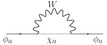
Figure 2: One loop self-energy for the active species to order $G^{2}$. The cut discontinuity across the $W-\chi$ lines yields the imaginary part $\mathrm{Im}\widetilde{\Sigma}_{aa}(k;\omega)$.

Because the bath fields are in thermal equilibrium, the noise correlation kernel $\widetilde{\mathcal{K}}_{\alpha\beta}(k;\omega)$ in eqn. (24) and the absorptive part of the retarded self energy $\mathrm{Im}\widetilde{\Sigma}_{\alpha\beta}(k;\omega)$ obey the generalized fluctuation dissipation relationhobos ; boyalamo ; hoboydavey

$$\widetilde{\mathcal{K}}_{\alpha\beta}(k;\omega)=\mathrm{Im}\widetilde{\Sigma}_{\alpha\beta}(k;\omega)\coth\left[\frac{\beta\omega}{2}\right]$$ (27)

The solution of the Langevin equation (23) ishobos ; boyalamo ; hoboydavey

$$\Psi_{\alpha,\vec{k}}(t)=\dot{G}_{\alpha\beta}(k;t)\,\Psi^{0}_{\beta,\vec{k}}+{G}_{\alpha\beta}(k;t)\,\Pi^{0}_{\beta,\vec{k}}+\int^{t}_{0}G_{\alpha\beta}(k;t^{\prime})~{}\xi_{\beta,\vec{k}}(t-t^{\prime})dt^{\prime}\,,$$ (28)

from which is clear that the propagator $G_{\alpha\beta}$ contains all the relevant information for the non-equilibrium dynamics.

In the Breit-Wigner (narrow width) approximation, the matrix propagator $G(k;t)$ in the flavor basis is given byhobos

$$G(k;t)= Z^{(1)}_{k}\,e^{-\frac{\Gamma_{1}(k)}{2}t}\,\Bigg{[}\frac{\sin(\Omega_{1}(k)t)}{{\Omega_{1}(k)}}\,\mathds{R}^{(1)}(\theta_{m})-\frac{\widetilde{\gamma}(k)}{2}\,\frac{\cos(\Omega_{1}(k)t)}{\Omega_{1}(k)}\,\mathds{R}^{(3)}(\theta_{m})\Bigg{]}+$$ (29)

$$Z^{(2)}_{k}\,e^{-\frac{\Gamma_{2}(k)}{2}t}\,\Bigg{[}\frac{\sin(\Omega_{2}(k)t)}{\Omega_{2}(k)}\,\mathds{R}^{(2)}(\theta_{m})+\frac{\widetilde{\gamma}(k)}{2}\,\frac{\cos(\Omega_{2}(k)t)}{\Omega_{2}(k)}\,\mathds{R}^{(3)}(\theta_{m})\Bigg{]}$$

where $Z^{(i)}_{k}$ are the residues at the quasiparticle poles and we have introduced the matrices

$$\mathds{R}^{(1)}(\theta)=\Bigg{(}\begin{array}[]{cc}\cos^{2}\theta&-\cos\theta\sin\theta\\ -\cos\theta\sin\theta&\sin^{2}\theta\\ \end{array}\Bigg{)}=U(\theta)\,\Bigg{(}\begin{array}[]{cc}1&0\\ 0&0\\ \end{array}\Bigg{)}\,U^{-1}(\theta)$$ (30)

$$\mathds{R}^{(2)}(\theta)=\Bigg{(}\begin{array}[]{cc}\sin^{2}\theta&\cos\theta\sin\theta\\ \cos\theta\sin\theta&\cos^{2}\theta\\ \end{array}\Bigg{)}=U(\theta)\,\Bigg{(}\begin{array}[]{cc}0&0\\ 0&1\\ \end{array}\Bigg{)}\,U^{-1}(\theta)$$ (31)

$$\mathds{R}^{(3)}(\theta)=\sin 2\theta~{}~{}\left(\begin{array}[]{cc}\sin 2\theta&\cos 2\theta\\ \cos 2\theta&-\sin 2\theta\\ \end{array}\right)=\sin 2\theta\,U(\theta)~{}\left(\begin{array}[]{cc}0&1\\ 1&0\\ \end{array}\right)~{}U^{-1}(\theta)\,.$$ (32)

From the results of referencehobos to leading order in $G$, the mixing angle in the medium is determined from the relations

$$\cos 2\theta_{m}=\frac{\cos 2\theta-\frac{V_{aa}}{\delta M^{2}}}{\varrho}~{}~{};~{}~{}\sin 2\theta_{m}=\frac{\sin 2\theta}{\varrho}\,,$$ (33)

where

$$\varrho=\Bigg{[}\big{(}\cos 2\theta-\frac{V_{aa}}{\delta M^{2}}\big{)}^{2}+\big{(}\sin 2\theta\big{)}^{2}\Bigg{]}^{\frac{1}{2}}\,.$$ (34)

The expressions (33) for the mixing angles in the medium in terms of the mixing angle in the vacuum and the matter potential is exactly of the same form as in the case of (fermionic) neutrinos in a mediumbook1 ; book2 ; book3 ; raffelt . An MSW resonance occurs wheneverbook1 ; book2 ; book3 ; raffelt

$$V_{aa}=\delta M^{2}\cos 2\theta\,.$$ (35)

The propagating frequencies and widths are given byhobos

$$\Omega_{1}(k) = \omega_{1}(k)+\Delta\omega_{1}(k)~{}~{};~{}~{}\Gamma_{1}(k)=\frac{\mathrm{Im}\widetilde{\Sigma}_{aa}(k;\omega_{1}(k))}{\omega_{1}(k)}~{}\cos^{2}\theta_{m}$$ (36)

$$\Omega_{2}(k) = \omega_{2}(k)+\Delta\omega_{2}(k)~{}~{};~{}~{}\Gamma_{2}(k)=\frac{\mathrm{Im}\widetilde{\Sigma}_{aa}(k;\omega_{2}(k))}{\omega_{2}(k)}~{}\sin^{2}\theta_{m}\,,$$ (37)

where

$$\omega^{2}_{1}(k) = k^{2}+\overline{M}^{2}+\frac{V_{aa}}{2}-\frac{\delta M^{2}\,\varrho}{2}$$ (38)

$$\omega^{2}_{2}(k) = k^{2}+\overline{M}^{2}+\frac{V_{aa}}{2}+\frac{\delta M^{2}\,\varrho}{2}$$ (39)

are the propagating frequencies (squared) in the medium including the matter potential at order $G$, namely the index of refraction arising from forward scattering, with $\overline{M}^{2}\,;\delta M^{2}$ defined in equation (7). The second order frequency shifts are

$$\Delta\omega_{1}(k) = -\frac{\cos^{2}\theta_{m}}{2\pi\omega_{1}(k)}\int d\omega\mathcal{P}\left[\frac{\mathrm{Im}\widetilde{\Sigma}_{aa}(k;\omega)}{\omega-\omega_{1}(k)}\right]\,$$ (40)

$$\Delta\omega_{2}(k) = -\frac{\sin^{2}\theta_{m}}{2\pi\omega_{2}(k)}\int d\omega\mathcal{P}\left[\frac{\mathrm{Im}\widetilde{\Sigma}_{aa}(k;\omega)}{\omega-\omega_{2}(k)}\right]\,\,,$$ (41)

andhobos

$$\widetilde{\gamma}(k)=\frac{\mathrm{Im}\widetilde{\Sigma}_{aa}(k;\overline{\omega}(k))}{\omega^{2}_{2}(k)-\omega^{2}_{1}(k)}~{}~{};~{}~{}\overline{\omega}(k)=\sqrt{k^{2}+\overline{M}^{2}}\,.$$ (42)

The relationship between the damping rates $\Gamma_{1,2}$ and the imaginary part of the self energy is the same as that obtained in the study of neutrinos with standard model interactions in a medium inhozeno .

To leading order in perturbation theory the denominator in equation (42) is $\delta M^{2}\rho$. When the matter potential dominates (at high temperature in the standard model), $V_{aa}\gg\delta M^{2}$ and $\delta M^{2}\rho\sim V_{aa}\propto G\gg\mathrm{Im}\widetilde{\Sigma}_{aa}\propto G^{2}$, thus in this regime $\widetilde{\gamma}\propto G\ll 1$. For example with active neutrinos with standard model interactions at high temperature, it was argued in ref.hozeno that $V_{aa}\propto G_{F}kT^{5}/M^{2}_{W}$ whereas $\mathrm{Im}\widetilde{\Sigma}_{aa}\sim G^{2}_{F}kT^{5}$ therefore at high temperature $\widetilde{\gamma}\sim\mathrm{Im}\widetilde{\Sigma}_{aa}/V_{aa}\sim g_{w}\ll 1$ with $g_{w}$ the standard model weak coupling.

In the opposite limit, for $\delta M^{2}\gg V_{aa}\propto G$ the vacuum mass difference dominates $\rho\sim 1$ and $\widetilde{\gamma}\ll 1$ since $\delta M^{2}\gg G\gg G^{2}$. This analysis is similar to that in ref.hozeno and precludes the possibility of “quantum zeno suppression”stodolsky ; kev1 at high temperature.

The only region in which $\widetilde{\gamma}$ may not be perturbatively small is near a resonance at which $\rho=|\sin 2\theta|$ and only for very small vacuum mixing angle so that $\delta M^{2}|\sin 2\theta|\propto G^{2}$. This situation requires a careful re-examination of the perturbative expansion, and in this case the propagator cannot be described as two separate Breit-Wigner resonances because the width of the resonances is of the same order of or larger than the separation between them. Such a possibility would require a complete re-assessment of the dynamics of the propagating modes in the medium as a consequence of the breakdown of the Breit-Wigner (or narrow width) approximation. However, for very small vacuum mixing angle, indeed a distinct possibility for $\mathrm{keV}$ sterile neutrinoskev1 , the MSW resonance is very narrow and in most of the parameter range $\widetilde{\gamma}\ll 1$ and can be safely neglected. This is certainly the case at very high or very low temperature regimes in which $V_{aa}\gg\delta M^{2}$ or $V_{aa}\ll\delta M^{2}$ respectively.

In summary, it follows from this discussion that $\widetilde{\gamma}(k)\ll 1$, with the possible exception near an MSW resonance for extremely small vacuum mixing anglehobos , and such a case must be studied in detail non-perturbatively.

Hence, neglecting perturbatively small corrections, the Green’s function in the flavor basis can be written as

$$G(k;t)=U(\theta_{m}(k))G_{m}(k;t)U^{-1}(\theta_{m}(k))$$ (43)

with

$$G_{m}(k;t)=\Bigg{(}\begin{array}[]{cc}e^{-\frac{\Gamma_{1}(k)}{2}t}~{}\frac{\sin(\Omega_{1}(k)t)}{{\Omega_{1}(k)}}&0\\ 0&e^{-\frac{\Gamma_{2}(k)}{2}t}~{}\frac{\sin(\Omega_{2}(k)t)}{{\Omega_{2}(k)}}\end{array}\Bigg{)}$$ (44)

This Green’s function and the expression for the damping rates $\Gamma_{1,2}$ in eqn. (36,37) lead to the following physical interpretation. The fields that diagonalize the Green’s function on the mass shell, namely $\phi_{1,2}$ are associated with the quasiparticle modes in the medium and describe the propagating excitations in the medium. From eqn. (43) these are related to the flavor fields $\phi_{a,s}$ by the unitary transformation

$$\phi_{a}=\cos\theta_{m}\phi_{1}+\sin\theta_{m}\phi_{2}~{}~{};~{}~{}\phi_{s}=\cos\theta_{m}\phi_{2}-\sin\theta_{m}\phi_{1}\,.$$ (45)

When the matter potential $V_{aa}\gg\delta M^{2}$, namely when $\theta_{m}\sim\pi/2$ it follows that $\phi_{a}\sim\phi_{2}$ and the damping rate of the active species is $\Gamma_{2}\sim\Gamma_{aa}$ while $\phi_{s}\sim\phi_{1}$ and the damping rate of the “sterile” species is $\Gamma_{1}\sim\Gamma_{aa}\cos^{2}\theta_{m}\ll\Gamma_{aa}$, where

$$\Gamma_{aa}\simeq\frac{\mathrm{Im}\widetilde{\Sigma}_{aa}(k;k)}{k}$$ (46)

is the ultrarelativistic limit of the damping rate of the active species in absence of mixing. In the opposite limit, when the medium mixing angle is small $\theta_{m}\sim 0$, corresponding to the near-vacuum case, $\phi_{a}\sim\phi_{1}$ and the active species has a damping rate $\Gamma_{1}\sim\Gamma_{aa}$ while $\phi_{s}\sim\phi_{2}$ with $\Gamma_{2}\sim\Gamma_{aa}\sin^{2}\theta_{m}\ll\Gamma_{aa}$. In both limits the sterile species is weakly coupled to the plasma, active and sterile species become equally coupled near an MSW resonance for $\theta_{m}\sim\pi/4$.

We emphasize that the relation (45) is not a relation between wave functions, but between the fields associated with the flavor eigenstates (active-sterile) and those associated with the propagating (quasiparticle) excitations in the medium (see section (V)).

III Quantum kinetics:

The distribution functions for the active $(a)$ and sterile $(s)$ species are defined in terms of the diagonal entries of the mass matrix in the flavor representation, namely

$$N_{\alpha}(k;t)=\frac{1}{2W_{\alpha}(k)}\Bigg{[}\langle\dot{\phi}_{\alpha}(\vec{k};t)\dot{\phi}_{\alpha}(-\vec{k},t)\rangle+W^{2}_{\alpha}(k)\langle{\phi}_{\alpha}(\vec{k};t){\phi}_{\alpha}(-\vec{k},t)\rangle\Bigg{]}-\frac{1}{2}~{}~{};~{}~{}\alpha=a,s$$ (47)

where

$$W^{2}_{\alpha}(k)=k^{2}+M^{2}_{\alpha\alpha}\,.$$ (48)

The equal time expectation values of Heisenberg field operators are in the initial density matrix, and as shown in referenceshobos ; boyalamo ; hoboydavey they are the same as the equal time expectation value of the center of mass Wigner variables $\Psi$, where the expectation value is now in terms of the initial density matrix for the system and the distribution function of the noise which is determined by the thermal bathhobos ; boyalamo ; hoboydavey . Therefore the distribution functions for the active and sterile species are given by

$$N_{\alpha}(k;t)=\frac{1}{2W_{\alpha}(k)}\Bigg{[}\langle\dot{\Psi}_{\alpha}(\vec{k};t)\dot{\Psi}_{\alpha}(-\vec{k},t)\rangle+W^{2}_{\alpha}(k)\langle{\Psi}_{\alpha}(\vec{k};t){\Psi}_{\alpha}(-\vec{k},t)\rangle\Bigg{]}-\frac{1}{2}~{}~{};~{}~{}\alpha=a,s$$ (49)

and the averages are taken over the initial density matrix of the system and the noise probability distribution. This expression combined with eqn.(28) makes manifest that the full time evolution of the distribution function is completely determined by the propagator $G_{\alpha\beta}(k,t)$ obtained from the solution of the effective equations of motion in the mediumhobos .

It proves convenient to introduce a matrix of distribution functions in terms of a parameter $\Omega$ as follows

$$\mathds{N}_{\alpha\beta}(k,t;\Omega)\equiv\frac{1}{2\Omega}\Bigg{[}\langle\dot{\Psi}_{\alpha}(\vec{k};t)\dot{\Psi}_{\beta}(-\vec{k},t)\rangle+\Omega^{2}\langle{\Psi}_{\alpha}(\vec{k};t){\Psi}_{\beta}(-\vec{k},t)\rangle\Bigg{]}-\frac{1}{2}\,\delta_{\alpha\beta}$$ (50)

from which we extract the active and sterile distribution functions from the diagonal elements, namely

$$N_{a}(k;t)=\mathds{N}_{a,a}(k,t;W_{a}(k))~{};~{}N_{s}(k;t)=\mathds{N}_{s,s}(k,t;W_{s}(k))$$ (51)

and the off-diagonal elements determine off-diagonal correlation functions of the fields and their canonical momenta in the flavor basis.

We consider first the initial density matrix for the system $\widehat{\rho}_{\Phi}(0)$ to be diagonal in the flavor basis with free field correlations

$$\mathrm{Tr}~{}\widehat{\rho}_{\Phi}(0)\Psi^{0}_{\alpha,\vec{k}}\Psi^{0}_{\beta,-\vec{k}}=\frac{1}{2W_{\alpha}(k)}\,\left[1+2N_{\alpha}(k;0)\right]\delta_{\alpha\beta}$$ (52)

$$\mathrm{Tr}~{}\widehat{\rho}_{\Phi}(0)\Pi^{0}_{\alpha,\vec{k}}\Pi^{0}_{\beta,-\vec{k}}=\frac{W_{\alpha}(k)}{2}\,\left[1+2N_{\alpha}(k;0)\right]\delta_{\alpha\beta}$$ (53)

$$\mathrm{Tr}~{}\widehat{\rho}_{\Phi}(0)\Psi^{0}_{\alpha,\vec{k}}\Pi^{0}_{\beta,-\vec{k}}=0$$ (54)

with $N_{\alpha}(k;0)$ being the initial distribution functions for the active and sterile species. Different initial conditions will be studied below.

Following the steps described in appendix (A) it is convenient to write $\mathds{N}(k,t;\Omega)=\mathds{N}^{(I)}(k,t;\Omega)+\mathds{N}^{(\xi)}(k,t;\Omega)$ where $\mathds{N}^{(I)}$ depends on the initial conditions but not on the noise $\xi$ and $\mathds{N}^{(\xi)}$ depends on the noise $\xi$ but not on the initial conditions. We find

$$\mathds{N}^{(I)}(k,t;\Omega) = \mathds{R}^{(1)}(\theta_{m})\,e^{-\Gamma_{1}t}\Bigg{\{}\cos^{2}(\theta_{m})\left[\frac{W^{2}_{a}+\Omega^{2}_{1}}{2W_{a}\Omega}\right]\left[\frac{1}{2}+N_{a}(0)\right]+\sin^{2}(\theta_{m})\left[\frac{W^{2}_{s}+\Omega^{2}_{1}}{2\Omega W_{s}}\right]\left[\frac{1}{2}+N_{s}(0)\right]\Bigg{\}}\left[\frac{\Omega^{2}+\Omega^{2}_{1}}{2\Omega^{2}_{1}}\right]$$ (55)

$$+ \mathds{R}^{(2)}(\theta_{m})\,e^{-\Gamma_{2}t}\Bigg{\{}\sin^{2}(\theta_{m})\left[\frac{W^{2}_{a}+\Omega^{2}_{2}}{2W_{a}\Omega}\right]\left[\frac{1}{2}+N_{a}(0)\right]+\cos^{2}(\theta_{m})\left[\frac{W^{2}_{s}+\Omega^{2}_{2}}{2\Omega W_{s}}\right]\left[\frac{1}{2}+N_{s}(0)\right]\Bigg{\}}\left[\frac{\Omega^{2}+\Omega^{2}_{2}}{2\Omega^{2}_{2}}\right]$$

$$+ \mathds{R}^{(3)}(\theta_{m})\,e^{-\frac{1}{2}(\Gamma_{1}+\Gamma_{2})t}\cos\left[(\Omega_{1}-\Omega_{2})t\right]\left[\frac{\Omega^{2}+\Omega_{2}\Omega_{1}}{4\Omega_{1}\Omega_{2}}\right]\Bigg{\{}\frac{(W_{a}-W_{s})}{4\Omega}\left(\frac{\Omega_{1}\Omega_{2}}{W_{a}W_{s}}-1\right)$$

$$+N_{a}(0)\left(\frac{\Omega_{1}\Omega_{2}+W^{2}_{a}}{2\Omega W_{a}}\right)-N_{s}(0)\left(\frac{\Omega_{1}\Omega_{2}+W^{2}_{s}}{2\Omega W_{s}}\right)\Bigg{\}}-\frac{\mathds{1}}{2}\,.$$

We have suppressed the dependence on $k$ to simplify the notation. The contribution from the noise term can be written as

$$\mathds{N}^{(\xi)}(k,t;\Omega)=\frac{1}{2\Omega}\int\frac{d\omega}{2\pi}U(\theta_{m})\Bigg{\{}h_{m}(\omega,t)\mathcal{K}_{m}(\omega)h^{*}_{m}(\omega,t)+\Omega^{2}f_{m}(\omega,t)\mathcal{K}_{m}(\omega)f^{*}_{m}(\omega,t)\Bigg{\}}U^{-1}(\theta_{m})$$ (56)

where

$$h_{m}(\omega,t)=\int_{0}^{t}e^{-i\omega t^{\prime}}G_{m}(k;t^{\prime})~{}~{};~{}~{}f_{m}(\omega,t)=\int_{0}^{t}e^{-i\omega t^{\prime}}\dot{G}_{m}(k;t^{\prime})$$ (57)

and

$$\mathcal{K}_{m}(\omega)=\mathrm{Im}\widetilde{\Sigma}_{aa}(k;\omega)\,\left[1+2n(\omega)\right]\Bigg{(}\begin{array}[]{cc}\cos^{2}(\theta_{m})&\cos(\theta_{m})\sin(\theta_{m})\\ \cos(\theta_{m})\sin(\theta_{m})&\sin^{2}(\theta_{m})\end{array}\Bigg{)}$$ (58)

After lengthy but straightforward algebra we find

$$\mathds{N}^{(\xi)}(k,t;\Omega)= \left[\frac{\Omega^{2}+\Omega^{2}_{1}}{2\Omega_{1}\Omega}\right]\left[\frac{1}{2}+n(\Omega_{1}(k))\right]\left(1-e^{-\Gamma_{1}(k)t}\right)\,\mathds{R}^{(1)}(\theta_{m}(k))+$$ (59)

$$\left[\frac{\Omega^{2}+\Omega^{2}_{2}}{2\Omega_{2}\Omega}\right]\left[\frac{1}{2}+n(\Omega_{2}(k))\right]\left(1-e^{-\Gamma_{2}(k)t}\right)\,\mathds{R}^{(2)}(\theta_{m}(k))$$

where we have neglected terms proportional to $\widetilde{\gamma}$.

Approximations: In arriving at the expressions (55), (59), we have made the following approximations:

• (a) We have taken $Z^{(i)}_{k}=1$ thus neglecting terms which are perturbatively small, of $\mathcal{O}(G^{2})$.

• (b) We have assumed $\Gamma_{i}/\Omega_{i}\ll 1$, which is warranted in perturbation theory and neglected terms proportional to this ratio.

• (c) As discussed above, consistently with perturbation theory we have assumed $\widetilde{\gamma}(k)\ll 1$ and neglected terms proportional to it. This corresponds to the interaction rate much smaller than the oscillation frequencies and relies on the consistency of the perturbative expansion.

• (d) In oscillatory terms we have taken a time average over the rapid time scales $1/\Omega_{1,2}$ replacing $\sin^{2}(\Omega_{1,2}t)=\cos^{2}(\Omega_{1,2}t)\rightarrow 1/2\,;\,\sin(\Omega_{1,2}t)=\cos(\Omega_{1,2}t)\rightarrow 0$.

Ultrarelativistic limit: The above expressions simplify considerably in the ultrarelativistic limit in which

$$\Omega\sim W_{a}(k)\sim W_{s}(k)\sim\Omega_{1}(k)\sim\Omega_{2}(k)\sim k\,,$$ (60)

and in this limit it follows that

$$\Gamma_{1}=\Gamma_{aa}\cos^{2}\theta_{m}~{};~{}\Gamma_{2}=\Gamma_{aa}\sin^{2}\theta_{m}$$ (61)

and $\Gamma_{aa}$ is the ultrarelativistic limit of the width of the active species in the absence of mixing given by eqn. (46). In this limit we obtain the following simple expression for the time evolution of the occupation number matrix in the flavor basis (suppressing the $k$ dependence for simplicity)

$$\mathds{N}(t) = \mathds{R}^{(1)}(\theta_{m})\Bigg{[}n(\Omega_{1})+\Big{(}N_{a}(0)\cos^{2}(\theta_{m})+N_{s}(0)\sin^{2}(\theta_{m})-n(\Omega_{1})\Big{)}\,e^{-\Gamma_{1}t}\Bigg{]}$$ (62)

$$+ \mathds{R}^{(2)}(\theta_{m})\Bigg{[}n(\Omega_{2})+\Big{(}N_{a}(0)\sin^{2}(\theta_{m})+N_{s}(0)\cos^{2}(\theta_{m})-n(\Omega_{2})\Big{)}\,e^{-\Gamma_{2}t}\Bigg{]}$$

$$+ \frac{1}{2}~{}\mathds{R}^{(3)}(\theta_{m})\,e^{-\frac{1}{2}(\Gamma_{1}+\Gamma_{2})t}\,\cos\left[(\Omega_{1}-\Omega_{2})t\right]\Big{(}N_{a}(0)-N_{s}(0)\Big{)}\,.$$

It is straightforward to verify that

$$\mathds{N}(0)=\left(\begin{array}[]{cc}N_{a}(0)&0\\ 0&N_{s}(0)\\ \end{array}\right)\,.$$ (63)

The active and sterile populations are given by the diagonal elements of (62), namely

$$N_{a}(t) = \cos^{2}(\theta_{m})\Bigg{[}n(\Omega_{1})+\Big{(}N_{a}(0)\cos^{2}(\theta_{m})+N_{s}(0)\sin^{2}(\theta_{m})-n(\Omega_{1})\Big{)}\,e^{-\Gamma_{1}t}\Bigg{]}$$ (64)

$$+ \sin^{2}(\theta_{m})\Bigg{[}n(\Omega_{2})+\Big{(}N_{a}(0)\sin^{2}(\theta_{m})+N_{s}(0)\cos^{2}(\theta_{m})-n(\Omega_{2})\Big{)}\,e^{-\Gamma_{2}t}\Bigg{]}$$

$$+ \frac{1}{2}~{}\sin^{2}(2\theta_{m})\,e^{-\frac{1}{2}(\Gamma_{1}+\Gamma_{2})t}\,\cos\left[(\Omega_{1}-\Omega_{2})t\right]\Big{(}N_{a}(0)-N_{s}(0)\Big{)}\,.$$

$$N_{s}(t) = \sin^{2}(\theta_{m})\Bigg{[}n(\Omega_{1})+\Big{(}N_{a}(0)\cos^{2}(\theta_{m})+N_{s}(0)\sin^{2}(\theta_{m})-n(\Omega_{1})\Big{)}\,e^{-\Gamma_{1}t}\Bigg{]}$$ (65)

$$+ \cos^{2}(\theta_{m})\Bigg{[}n(\Omega_{2})+\Big{(}N_{a}(0)\sin^{2}(\theta_{m})+N_{s}(0)\cos^{2}(\theta_{m})-n(\Omega_{2})\Big{)}\,e^{-\Gamma_{2}t}\Bigg{]}$$

$$- \frac{1}{2}~{}\sin^{2}(2\theta_{m})\,e^{-\frac{1}{2}(\Gamma_{1}+\Gamma_{2})t}\,\cos\left[(\Omega_{1}-\Omega_{2})t\right]\left(N_{a}(0)-N_{s}(0)\right)\,.$$

The oscillatory term which results from the interference of the propagating modes $1,2$ damps out with a damping factor

$$\frac{1}{2}(\Gamma_{1}+\Gamma_{2})=\frac{\Gamma_{aa}}{2}$$ (66)

which determines the decoherence time scale $\tau_{dec}=2/\Gamma_{aa}$. These expressions are one of the main results of this article.

Initial density matrix diagonal in the $1-2$ basis: The above results were obtained assuming that the initial density matrix is diagonal in the flavor basis, if instead, it is diagonal in the basis of the propagating modes in the medium, namely the $1-2$ basis, it is straightforward to find the result

$$\mathds{N}(t)= U(\theta_{m})\Bigg{\{}\left(\begin{array}[]{cc}1&0\\ 0&0\\ \end{array}\right)\Bigg{[}n(\Omega_{1})+\Big{(}N_{1}(0)-n(\Omega_{1})\Big{)}\,e^{-\Gamma_{1}t}\Bigg{]}$$ (72)

$$+\left(\begin{array}[]{cc}0&0\\ 0&1\\ \end{array}\right)\Bigg{[}n(\Omega_{2})+\Big{(}N_{2}(0)-n(\Omega_{2})\Big{)}\,e^{-\Gamma_{2}t}\Bigg{]}\Bigg{\}}U^{-1}(\theta_{m})\,.$$

In particular, the active and sterile distribution functions become

$$N_{a}(t) = \cos^{2}\theta_{m}\Bigg{[}n(\Omega_{1})+\Big{(}N_{1}(0)-n(\Omega_{1})\Big{)}\,e^{-\Gamma_{1}t}\Bigg{]}+\sin^{2}\theta_{m}\Bigg{[}n(\Omega_{2})+\Big{(}N_{2}(0)-n(\Omega_{2})\Big{)}\,e^{-\Gamma_{2}t}\Bigg{]}$$ (73)

$$N_{s}(t) = \cos^{2}\theta_{m}\Bigg{[}n(\Omega_{2})+\Big{(}N_{2}(0)-n(\Omega_{2})\Big{)}\,e^{-\Gamma_{2}t}\Bigg{]}+\sin^{2}\theta_{m}\Bigg{[}n(\Omega_{1})+\Big{(}N_{1}(0)-n(\Omega_{1})\Big{)}\,e^{-\Gamma_{1}t}\Bigg{]}\,.$$ (74)

The results summarized by eqns. (64-74) show that the distribution functions for the propagating modes in the medium, namely the $1,2$ quasiparticles, reach equilibrium with the damping factor $\Gamma_{1,2}$ which is twice the damping rate of the quasiparticle modes (see eqn. (44)). The interference term is present only when the initial density matrix is off diagonal in the (1,2) basis of propagating modes in the medium.

If the initial density matrix is off-diagonal in the (1,2) basis, these off diagonal components damp-out within the decoherence time scale $\tau_{dec}$, while the diagonal elements attain the values of the equilibrium distributions on the time scales $1/\Gamma_{1},1/\Gamma_{2}$.

IV The Quantum Master equation

The quantum master equation is the equation of motion of the reduced density matrix of the system fields in the interaction picture after integrating out the bath degrees of freedom. The first step is to define the interaction picture, for which a precise separation between the free and interaction parts in the Hamiltonian is neededqobooks . In order to carry out the perturbative expansion in terms of the eigenstates in the medium, we include the lowest order forward scattering correction, namely the index of refraction into the un-perturbed Hamiltonian. This is achieved by writing the term

$$\phi^{2}_{a}\chi^{2}=\phi^{2}_{a}\langle\chi^{2}\rangle+\phi^{2}_{a}\delta\chi^{2}$$ (75)

where

$$\delta\chi^{2}=\chi^{2}-\langle\chi^{2}\rangle~{}~{};~{}~{}\langle\delta\chi^{2}\rangle=0$$ (76)

and the average is performed in the bath density matrix $\rho_{B}(0)=e^{-\beta H_{0}[\chi,W]}$. In this manner the quadratic part of the Lagrangian density for the active and sterile fields is

$$\mathcal{L}_{0}[\phi]=\frac{1}{2}\left\{\partial_{\mu}\Phi^{T}\partial^{\mu}\Phi-\Phi^{T}(\mathds{M}^{2}+\mathds{V})\Phi\right\}$$ (77)

where $\mathds{V}$ is the matter potential given by eqn. (21). The unperturbed Hamiltonian for the system fields in the medium is diagonalized by the unitary transformation (4) but with the unitary matrix $U(\theta_{m})$ with $\theta_{m}$ being the mixing angle in the medium given by equations (33,34) and $\varphi_{1},\varphi_{2}$ are now the fields associated with the eigenstates of the Hamiltonian in the medium including the index of refraction correction from the matter potential to $\mathcal{O}(G)$ ($\mathcal{O}(G_{F})$ in the case of neutrinos with standard model interactions). Introducing creation and annihilation operators for the fields $\varphi_{1,2}$ with usual canonical commutation relations, the unperturbed Hamiltonian for the propagating modes in the medium including the index of refraction is

$$H_{S}[\varphi_{1,2}]=\sum_{\vec{k}}\sum_{i=1,2}\left[a^{\dagger}_{i}(\vec{k})a_{i}(\vec{k})\omega_{i}(k)\right]$$ (78)

where $\omega_{i}(k)$ are the propagating frequencies in the medium given in equation (38,39). The interaction Hamiltonian is

$$H_{I}=G\int d^{3}x\left[\phi^{2}_{a}\delta\chi^{2}+\phi_{a}\mathcal{O}_{a}\right]$$ (79)

where

$$\phi_{a}=\cos(\theta_{m})\varphi_{1}+\sin(\theta_{m})\varphi_{2}\,.$$ (80)

This formulation represents a re-arrangement of the perturbative expansion in terms of the fields that create and annihilate the propagating modes in the medium. The remaining steps are available in the quantum optics literatureqobooks . Denoting the Hamiltonian for the bath degrees of freedom $H_{0}[\chi,W]\equiv H_{B}$ the total Hamiltonian is $H=H_{S}+H_{B}+H_{I}\equiv\overline{H}_{0}+H_{I}$. The density matrix in the interaction picture is

$$\widehat{\rho}_{i}(t)=e^{i\overline{H}_{0}t}\widehat{\rho}(t)e^{-i\overline{H}_{0}t}$$ (81)

where $\widehat{\rho}(t)$ is given by eqn. (13) and it obeys the equation of motion

$$\frac{d\widehat{\rho}_{i}(t)}{dt}=-i\left[H_{I}(t),\widehat{\rho}_{i}(t)\right]$$ (82)

with $H_{I}(t)=e^{i\overline{H}_{0}t}H_{I}e^{-i\overline{H}_{0}t}$ is the interaction Hamiltonian in the interaction picture of $\overline{H}_{0}$. Iteration of this equation up to second order in the interaction yieldsqobooks

$$\frac{d\widehat{\rho}_{i}(t)}{dt}=-i\left[H_{I}(t),\widehat{\rho}_{i}(0)\right]-\int^{t}_{0}dt^{\prime}\left[H_{I}(t),\left[H_{I}(t^{\prime}),\widehat{\rho}_{i}(t^{\prime})\right]\right]+\cdots$$ (83)

The reduced density matrix for the system is obtained from the total density matrix by tracing over the bath degrees of freedom which are assumed to remain in equilibriumqobooks . At this stage, several standard approximations are invokedqobooks :

• i): factorization: the total density matrix is assumed to factorize

  $$\widehat{\rho}_{i}(t)=\rho_{S,i}(t)\otimes\rho_{B}(0)$$ (84)

  where it is assumed that the bath remains in equilibrium, this approximation is consistent with obtaining the effective action by tracing over the bath degrees of freedom with an equilibrium thermal density matrix. The correlation functions of the bath degrees of freedom are not modified by the coupling to the system.

• ii): Markovian approximation: the memory of the evolution is neglected and in the double commutator in (83) $\widehat{\rho}_{i}(t^{\prime})$ is replaced by $\widehat{\rho}_{i}(t)$ and taken out of the integral.

Taking the trace over the bath degrees of freedom yields the quantum master equation for the reduced density matrix,

$$\frac{d{\rho}_{S,i}(t)}{dt}=-\int^{t}_{0}dt^{\prime}{\mathrm{Tr}}_{B}\big{\{}\left[H_{I}(t),\left[H_{I}(t^{\prime}),\widehat{\rho}_{i}(t)\right]\right]\big{\}}+\cdots$$ (85)

where the first term has vanished by dint of the fact that the matter potential was absorbed into the unperturbed Hamiltonian, namely $Tr_{B}\rho_{B}(0)\delta\chi^{2}=0$. This is an important aspect of the interaction picture in the basis of the propagating states in the medium. Up to second order we will only consider the interaction term

$$H_{I}(t)=\sum_{\vec{k}}\left[\cos\theta_{m}\varphi_{1,\vec{k}}(t)+\sin\theta_{m}\varphi_{2,\vec{k}}(t)\right]\mathcal{O}_{-\vec{k}}(t)$$ (86)

where we have written the interaction Hamiltonian in terms of spatial Fourier transforms and the fields are in the interaction picture of $\overline{H}_{0}$. We neglect non-linearities from the second order contributions of the term $\phi^{2}_{a}\delta\chi^{2}$, the non-linearities associated with the neutrino background are included in the forward scattering corrections accounted for in the matter potential. The quartic non-linearities are associated with active “neutrino-neutrino” elastic scattering and are not relevant for the production of the sterile species.

The next steps are: i) writing out explicitly the nested commutator in (85) yielding four different terms, ii) taking the trace over the bath degrees of freedom yielding the correlation functions of the bath operators $Tr_{B}\mathcal{O}(t)\mathcal{O}(t^{\prime})$ (and $t\leftrightarrow t^{\prime}$) and, iii) carrying out the integrals in the variable $t^{\prime}$. While straightforward these steps are lengthy and technical and are relegated to appendix (B). Two further approximations are invokedqobooks ,

• iii): the “rotating wave approximation”: terms that feature rapidly varying phases of the form $e^{\pm 2i\omega_{1,2}t};e^{\pm i(\omega_{1}+\omega_{2})t}$ are averaged out in time leading to their cancellation. This approximation also has a counterpart in the effective action approach in the averaging of rapidly varying terms, see the discussion after equation (59).

• iv): the Wigner Weisskopf approximation: time integrals of the form

  $$\int^{t}_{0}e^{-i(\omega-\Omega)\tau}d\tau\approx-i\mathcal{P}\left[\frac{1}{\omega-\Omega}\right]+\pi\delta(\omega-\Omega)\,$$ (87)

  where $\mathcal{P}$ stands for the principal part. The Markovian approximation (ii) when combined with the Wigner-Weisskopf approximation is equivalent to approximating the propagators by their narrow width Breit-Wigner form in the effective action.

All of these approximations i)- iv) detailed above are standard in the derivation of quantum master equations in the literatureqobooks .

The quantum master equation is obtained in appendix (B), it features diagonal and off-diagonal terms in the $1-2$ basis and is of the Lindblad formqobooks which ensures that the trace of the reduced density matrix is a constant of motion as it must be, because it is consistently derived from the full Liouville evolution (13). We now focus on the ultrarelativistic case $\omega_{1}(k)\sim\omega_{2}(k)\sim k$ which leads to substantial simplifications and is the relevant case for sterile neutrinos in the early Universe, we also neglect the second order corrections to the propagation frequencies. With these simplifications we obtain,

$$\frac{d{\rho}_{S,i}}{dt} = \Bigg{\{}\sum_{j=1,2}\sum_{\vec{k}}-\frac{\Gamma_{j}(k)}{2}\Bigg{[}\big{[}1+n(\omega_{j}(k))\big{]}\bigg{(}\rho_{S,i}a^{\dagger}_{j}(\vec{k})a_{j}(\vec{k})+a^{\dagger}_{j}(\vec{k})a_{j}(\vec{k})\rho_{S,i}-2a_{j}(\vec{k})\rho_{S,i}a^{\dagger}_{j}(\vec{k})\bigg{)}$$ (88)

$$+ n(\omega_{j}(k))\bigg{(}\rho_{S,i}a_{j}(\vec{k})a^{\dagger}_{j}(\vec{k})+a_{j}(\vec{k})a^{\dagger}_{j}(\vec{k})\rho_{S,i}-2a^{\dagger}_{j}(\vec{k})\rho_{S,i}a_{j}(\vec{k})\bigg{)}\Bigg{]}$$

$$- \sum_{\vec{k}}\frac{\widetilde{\Gamma}(k)}{2}\Bigg{\{}\Bigg{[}\Big{(}1+n(\omega_{1}(k))\Big{)}\Big{(}a^{\dagger}_{2}(k;t)a_{1}(k;t)\rho_{S,i}+\rho_{S,i}a^{\dagger}_{1}(k;t)a_{2}(k;t)-a_{2}(k;t)\rho_{S,i}a^{\dagger}_{1}(k;t)$$

$$- a_{1}(k;t)\rho_{S,i}a^{\dagger}_{2}(k;t)\Big{)}+n(\omega_{1}(k))\Big{(}a_{2}(k;t)a^{\dagger}_{1}(k;t)\rho_{S,i}+\rho_{S,i}a_{1}(k;t)a^{\dagger}_{2}(k;t)-a^{\dagger}_{2}(k;t)\rho_{S,i}a_{1}(k;t)$$

$$- a^{\dagger}_{1}(k;t)\rho_{S,i}a_{2}(k;t)\Big{)}\Bigg{]}+\Bigg{[}\Big{(}1+n(\omega_{2}(k))\Big{)}\Big{(}a^{\dagger}_{1}(k;t)a_{2}(k;t)\rho_{S,i}+\rho_{S,i}a^{\dagger}_{2}(k;t)a_{1}(k;t)-a_{1}(k;t)\rho_{S,i}a^{\dagger}_{2}(k;t)$$

$$- a_{2}(k;t)\rho_{S,i}a^{\dagger}_{1}(k;t)\Big{)}+n(\omega_{2}(k))\Big{(}a_{1}(k;t)a^{\dagger}_{2}(k;t)\rho_{S,i}+\rho_{S,i}a_{2}(k;t)a^{\dagger}_{1}(k;t)-a^{\dagger}_{1}(k;t)\rho_{S,i}a_{2}(k;t)$$

$$- a^{\dagger}_{2}(k;t)\rho_{S,i}a_{1}(k;t)\Big{)}\Bigg{]}\Bigg{\}}\,,$$

where

$$\Gamma_{1}(k)=\Gamma_{aa}(k)\cos^{2}\theta_{m}~{}~{},~{}~{}\Gamma_{2}(k)=\Gamma_{aa}(k)\sin^{2}\theta_{m}$$

$$\widetilde{\Gamma}(k)=\frac{1}{2}\sin 2\theta_{m}\Gamma_{aa}(k)~{}~{};~{}~{}\Gamma_{aa}(k)=\frac{\mathrm{Im}\Sigma_{aa}(k,k)}{k}$$ (89)

and the interaction picture operators are given in eqn. (186). The expectation value of any system’s operator $A$ is given by

$$\langle A\rangle(t)=\mathrm{Tr}\rho_{i,S}(t)A(t)$$ (90)

where $A(t)$ is the operator in the interaction picture of $\overline{H}_{0}$, thus the time derivative of this expectation value contains two contributions

$$\frac{d}{dt}\langle A\rangle(t)=\mathrm{Tr}\dot{\rho}_{i,S}(t)A(t)+\mathrm{Tr}\rho_{i,S}(t)\dot{A}(t)\,.$$ (91)

The distribution functions for active and sterile species is defined as in equation (49) with the averages defined as in (90), namely

$$N_{\alpha}(k;t)=\mathrm{Tr}\rho_{i,S}(t)\Bigg{[}\frac{\dot{\phi}_{\alpha}(\vec{k};t)\dot{\phi}_{\alpha}(-\vec{k},t)}{2W_{\alpha}(k)}+\frac{W_{\alpha}(k)}{2}~{}{\phi}_{\alpha}(\vec{k};t){\phi}_{\alpha}(-\vec{k},t)\Bigg{]}-\frac{1}{2}\,,$$ (92)

where the fields are in the interaction picture of $\overline{H}_{0}$. The active and sterile fields are related to the fields that create and annihilate the propagating modes in the medium as

$$\phi_{a}(\vec{k})=\cos\theta_{m}\varphi_{1}(\vec{k})+\sin\theta_{m}\varphi_{2}(\vec{k})~{}~{};~{}~{}\phi_{s}(\vec{k})=\cos\theta_{m}\varphi_{2}(\vec{k})-\sin\theta_{m}\varphi_{1}(\vec{k})\,.$$ (93)

In the interaction picture of $\overline{H}_{0}$

$$\varphi_{j}(\vec{k},t)=\frac{1}{\sqrt{2\omega_{j}(k)}}\Bigg{[}a_{j}(\vec{k})~{}e^{-i\omega_{j}(k)t}+a^{\dagger}_{j}(-\vec{k})~{}e^{i\omega_{j}(k)t}\Bigg{]}$$ (94)

where $\omega_{j}(k)$ are the propagation frequencies in the medium up to leading order in $G$, given by equations (38,39). Introducing this expansion into the expression (92) we encounter the ratio of the propagating frequencies in the medium $\omega_{j}$ and the bare frequencies $W_{\alpha}$. Just as we did in the previous section, we focus on the relevant case of ultrarelativistic species and approximate as in equation (60) $\omega_{j}(k)\sim W_{\alpha}(k)\sim k$, in which case we find the relation between the creation-annihilation operators for the flavor fields and those of the $1,2$ fields to behobos

$$a_{a}(\vec{k},t)=\cos\theta_{m}a_{1}(\vec{k},t)+\sin\theta_{m}a_{2}(\vec{k},t)~{}~{};~{}~{}a_{s}(\vec{k},t)=\cos\theta_{m}a_{2}(\vec{k},t)-\sin\theta_{m}a_{1}(\vec{k},t)$$ (95)

leading to the simpler expressions for the active and sterile distributions,

$$N_{a}(k;t)=\mathrm{Tr}\rho_{i,S}(t)\Bigg{[} \cos^{2}\theta_{m}a^{\dagger}_{1}(\vec{k},t)a_{1}(\vec{k},t)+\sin^{2}\theta_{m}a^{\dagger}_{2}(\vec{k},t)a_{2}(\vec{k},t)$$ (96)

$$+\frac{1}{2}\sin 2\theta_{m}(a^{\dagger}_{1}(\vec{k},t)a_{2}(\vec{k},t)+a^{\dagger}_{2}(\vec{k},t)a_{1}(\vec{k},t))\Bigg{]}$$

$$N_{s}(k;t)=\mathrm{Tr}\rho_{i,S}(t)\Bigg{[} \cos^{2}\theta_{m}a^{\dagger}_{2}(\vec{k},t)a_{2}(\vec{k},t)+\sin^{2}\theta_{m}a^{\dagger}_{1}(\vec{k},t)a_{1}(\vec{k},t)$$ (97)

$$-\frac{1}{2}\sin 2\theta_{m}(a^{\dagger}_{1}(\vec{k},t)a_{2}(\vec{k},t)+a^{\dagger}_{2}(\vec{k},t)a_{1}(\vec{k},t))\Bigg{]}\,.$$

In the interaction picture of $\overline{H}_{0}$ the products $a^{\dagger}_{j}(\vec{k},t)a_{j}(\vec{k},t)$ are time independent and $a^{\dagger}_{1}(\vec{k},t)a_{2}(\vec{k},t)=a^{\dagger}_{1}(\vec{k},0)a_{2}(\vec{k},0)~{}e^{i(\omega_{1}(k)-\omega_{2}(k))t}$. It is convenient to introduce the distribution functions and off-diagonal correlators

$$n_{11}(k,t)=\mathrm{Tr}\rho_{i,S}(t)a^{\dagger}_{1}(k,t)a_{1}(k,t)~{}~{},~{}~{}n_{22}(k,t)=\mathrm{Tr}\rho_{i,S}(t)a^{\dagger}_{2}(k,t)a_{2}(k,t)$$ (98)

$$n_{12}(k,t)=\mathrm{Tr}\rho_{i,S}(t)a^{\dagger}_{1}(k,t)a_{2}(k,t)~{}~{},~{}~{}n_{21}(k,t)=\mathrm{Tr}\rho_{i,S}(t)a^{\dagger}_{2}(k,t)a_{1}(k,t)=n^{*}_{12}(k,t)\,.$$ (99)

In terms of these, the distribution functions for the active and sterile species in the ultrarelativistic limit becomes

$$N_{a}(k;t) = \cos^{2}\theta_{m}n_{11}(k;t)+\sin^{2}\theta_{m}n_{22}(k;t)+\frac{1}{2}\sin 2\theta_{m}\Big{(}n_{12}(k;t)+n_{21}(k;t)\Big{)}$$ (100)

$$N_{s}(k;t) = \sin^{2}\theta_{m}n_{11}(k;t)+\cos^{2}\theta_{m}n_{22}(k;t)-\frac{1}{2}\sin 2\theta_{m}\Big{(}n_{12}(k;t)+n_{21}(k;t)\Big{)}\,.$$ (101)

From eqn. (91) we obtain the following kinetic equations for $n_{ij}(k;t)$

$$\dot{n}_{11} = -\Gamma_{1}\Big{[}n_{11}-n_{eq,1}\Big{]}-\frac{\widetilde{\Gamma}}{2}\Big{[}n_{12}+n_{21}\Big{]}$$ (102)

$$\dot{n}_{22} = -\Gamma_{2}\Big{[}n_{22}-n_{eq,2}\Big{]}-\frac{\widetilde{\Gamma}}{2}\Big{[}n_{12}+n_{21}\Big{]}$$ (103)

$$\dot{n}_{12} = \Big{[}-i\Delta\omega-\frac{\Gamma_{aa}}{2}\Big{]}n_{12}-\frac{\widetilde{\Gamma}}{2}\Big{[}(n_{11}-n_{eq,1})+(n_{22}-n_{eq,2})\Big{]}$$ (104)

$$\dot{n}_{21} = \Big{[}+i\Delta\omega-\frac{\Gamma_{aa}}{2}\Big{]}n_{21}-\frac{\widetilde{\Gamma}}{2}\Big{[}(n_{11}-n_{eq,1})+(n_{22}-n_{eq,2})\Big{]}\,,$$ (105)

where $n_{eq,j}=n(\omega_{j}(k))$ are the equilibrium distribution functions for the corresponding propagating modes, and $\Delta\omega=(\omega_{2}(k)-\omega_{1}(k))$. As we have argued above, in perturbation theory $\Gamma_{aa}(k)/\Delta\omega(k)\ll 1$, which is the same statement as the approximation $\widetilde{\gamma}\ll 1$ as discussed for the effective action, and in this case the off diagonal contributions to the kinetic equations yield perturbative corrections to the distribution functions and correlators. To leading order in this ratio we find the distribution functions,

$$n_{11}(t)=n_{eq,1}+\Big{(}n_{11}(0)-n_{eq,1}\Big{)}~{}e^{-\Gamma_{1}t}-\frac{\widetilde{\Gamma}e^{-\Gamma_{1}t}}{2\Delta\omega}\Bigg{[}i~{}n_{12}(0)\Big{[}e^{-i\Delta\omega t}~{}e^{\frac{1}{2}(\Gamma_{2}-\Gamma_{1})t}-1\Big{]}+c.c.\Bigg{]}$$ (106)

$$n_{22}(t)=n_{eq,2}+\Big{(}n_{22}(0)-n_{eq,2}\Big{)}~{}e^{-\Gamma_{2}t}-\frac{\widetilde{\Gamma}e^{-\Gamma_{2}t}}{2\Delta\omega}\Bigg{[}i~{}n_{12}(0)\Big{[}e^{-i\Delta\omega t}~{}e^{\frac{1}{2}(\Gamma_{1}-\Gamma_{2})t}-1\Big{]}+c.c.\Bigg{]}$$ (107)

and off-diagonal correlators

$$n_{12}(t) = e^{-i\Delta\omega t}~{}e^{-\frac{\Gamma_{aa}}{2}t}~{}\Bigg{\{}n_{12}(0)+i\frac{\widetilde{\Gamma}}{2\Delta\omega}\Bigg{[}(n_{11}(0)-n_{eq,1})\Big{[}e^{i\Delta\omega t}~{}e^{\frac{1}{2}(\Gamma_{2}-\Gamma_{1})t}-1\Big{]}$$ (108)

$$+ (n_{22}(0)-n_{eq,2})\Big{[}e^{i\Delta\omega t}~{}e^{\frac{1}{2}(\Gamma_{1}-\Gamma_{2})t}-1\Big{]}\Bigg{]}\Bigg{\}}$$

where

$$\frac{\widetilde{\Gamma}}{2\Delta\omega}=\frac{1}{2}\sin 2\theta_{m}\frac{\mathrm{Im}\Sigma_{aa}(k,k)}{2k(\omega_{2}(k)-\omega_{1}(k)}=\frac{1}{2}\sin 2\theta_{m}\widetilde{\gamma}$$ (109)

with $\widetilde{\gamma}$ defined in eqn. (42) and we have suppressed the momenta index for notational convenience.

IV.1 Comparing the effective action and quantum master equation

We can now establish the equivalence between the time evolution of the distribution functions obtained from the effective action and the quantum master equation, however in order to compare the results we must first determine the initial conditions in equations (106-108). The initial values $n_{ij}(0)$ must be determined from the initial condition and depend on the initial density matrix. Two important cases stand out: i) an initial density matrix diagonal in the flavor basis or ii) diagonal in the $1-2$ basis of propagating eigenstates in the medium.

Initial density matrix diagonal in the flavor basis: the initial expectation values are obtained by inverting the relation between $\varphi_{1,2}$ and $\phi_{a,s}$. We obtain

$$n_{11}(0)=\langle a^{\dagger}_{1}(\vec{k})a_{1}(\vec{k})\rangle(0) = \cos^{2}\theta_{m}N_{a}(0)+\sin^{2}\theta_{m}N_{s}(0)$$ (110)

$$n_{22}(0)=\langle a^{\dagger}_{2}(\vec{k})a_{2}(\vec{k})\rangle(0) = \cos^{2}\theta_{m}N_{s}(0)+\sin^{2}\theta_{m}N_{a}(0)$$ (111)

$$n_{12}(0)=\langle a^{\dagger}_{1}(\vec{k})a_{2}(\vec{k})\rangle(0) = \frac{1}{2}\sin 2\theta_{m}(N_{a}(0)-N_{s}(0))$$ (112)

It is straightforward to establish the equivalence between the results obtained from the effective action and those obtained above from the quantum master equation as follows: i) neglect the second order frequency shifts ($\Omega_{1,2}\sim\omega_{1,2}$) and the perturbatively small corrections of order $\widetilde{\gamma}$, ii) insert the initial conditions (110-112) in the solutions (106-108), finally using the relations (100,101) for the active and sterile distribution functions we find precisely the results given by equations (64,65) obtained via the non-equilibrium effective action.

Initial density matrix diagonal in the $1-2$ basis: in this case

$$\langle a^{\dagger}_{1}(\vec{k})a_{1}(\vec{k})\rangle(0) = N_{1}(0)$$

$$\langle a^{\dagger}_{2}(\vec{k})a_{2}(\vec{k})\rangle(0) = N_{2}(0)$$

$$\langle a^{\dagger}_{1}(\vec{k})a_{2}(\vec{k})\rangle(0) = 0$$ (113)

with these initial conditions it is straightforward to obtain the result (73,74).

The fundamental advantage in the method of the effective action is that it highlights that the main ingredient is the full propagator in the medium and the emerging time scales for the time evolution of distribution functions and coherences are completely determined by the quasiparticle dispersion relations and damping rates.

IV.2 Quantum kinetic equations: summary

Having confirmed the validity of the kinetic equations via two independent but complementary methods, we now summarize the quantum kinetic equations in a form amenable to numerical study. For this purpose it is convenient to define the hermitian combinations

$$n_{R}(t)=n_{12}(t)+n_{21}(t)~{};~{}n_{I}(t)=i(n_{12}(t)-n_{21}(t))$$ (114)

in terms of which the quantum kinetic equations for the distribution functions and coherences become (suppressing the momentum label)

$$\dot{n}_{11} = -\Gamma_{aa}\cos^{2}\theta_{m}\Big{[}n_{11}-n_{eq,1}\Big{]}-\frac{\Gamma_{aa}}{4}\sin 2\theta_{m}~{}n_{R}$$ (115)

$$\dot{n}_{22} = -\Gamma_{aa}\sin^{2}\theta_{m}\Big{[}n_{22}-n_{eq,2}\Big{]}-\frac{\Gamma_{aa}}{4}\sin 2\theta_{m}~{}n_{R}$$ (116)

$$\dot{n}_{R} = -(\omega_{2}-\omega_{1})~{}n_{I}-\frac{\Gamma_{aa}}{2}n_{R}-\frac{\Gamma_{aa}}{2}\sin 2\theta_{m}\Big{[}(n_{11}-n_{eq,1})+(n_{22}-n_{eq,2})\Big{]}$$ (117)

$$\dot{n}_{I} = (\omega_{2}-\omega_{1})~{}n_{R}-\frac{\Gamma_{aa}}{2}n_{I}\,,$$ (118)

with the active and sterile distribution functions related to the quantities above as follows

$$N_{a}(k;t) = \cos^{2}\theta_{m}n_{11}(k;t)+\sin^{2}\theta_{m}n_{22}(k;t)+\frac{1}{2}\sin 2\theta_{m}n_{R}(k;t)$$ (119)

$$N_{s}(k;t) = \sin^{2}\theta_{m}n_{11}(k;t)+\cos^{2}\theta_{m}n_{22}(k;t)-\frac{1}{2}\sin 2\theta_{m}n_{R}(k;t)\,.$$ (120)

In the perturbative limit when $\Gamma_{aa}\sin 2\theta_{m}/\Delta\omega\ll 1$ which as argued above is the correct limit in all but for a possible small region near an MSW resonancehozeno , the set of kinetic equations simplify to

$$\dot{n}_{11} = -\Gamma_{aa}\cos^{2}\theta_{m}\Big{[}n_{11}-n_{eq,1}\Big{]}$$ (121)

$$\dot{n}_{22} = -\Gamma_{aa}\sin^{2}\theta_{m}\Big{[}n_{22}-n_{eq,2}\Big{]}$$ (122)

$$\dot{n}_{R} = -\Big{(}\omega_{2}-\omega_{1}\Big{)}~{}n_{I}-\frac{\Gamma_{aa}}{2}n_{R}$$ (123)

$$\dot{n}_{I} = \Big{(}\omega_{2}-\omega_{1}\Big{)}~{}n_{R}-\frac{\Gamma_{aa}}{2}n_{I}\,.$$ (124)

In this case the active and sterile populations are given by (suppressing the momentum variable)

$$N_{a}(t) = \cos^{2}(\theta_{m})\Bigg{[}n_{eq}(\omega_{1})+\Big{(}n_{11}(0)-n_{eq}(\omega_{1})\Big{)}\,e^{-\Gamma_{1}t}\Bigg{]}$$ (125)

$$+ \sin^{2}(\theta_{m})\Bigg{[}n_{eq}(\omega_{2})+\Big{(}n_{22}(0)-n_{eq}(\omega_{2})\Big{)}\,e^{-\Gamma_{2}t}\Bigg{]}$$

$$+ ~{}\sin(2\theta_{m})\,e^{-\frac{\Gamma_{aa}}{2}t}\,\cos\left[(\omega_{1}-\omega_{2})t\right]~{}n_{12}(0)\,.$$

$$N_{s}(t) = \sin^{2}(\theta_{m})\Bigg{[}n_{eq}(\omega_{1})+\Big{(}n_{11}(0)-n_{eq}(\omega_{1})\Big{)}\,e^{-\Gamma_{1}t}\Bigg{]}$$ (126)

$$+ \cos^{2}(\theta_{m})\Bigg{[}n_{eq}(\omega_{2})+\Big{(}n_{22}(0)-n_{eq}(\omega_{2})\Big{)}\,e^{-\Gamma_{2}t}\Bigg{]}$$

$$- ~{}\sin(2\theta_{m})\,e^{-\frac{\Gamma_{aa}}{2}t}\,\cos\left[(\omega_{1}-\omega_{2})t\right]~{}n_{12}(0)\,,$$

where

$$\Gamma_{1}(k)=\Gamma_{aa}(k)\cos^{2}\theta_{m}~{}~{};~{}~{}\Gamma_{2}(k)=\Gamma_{aa}(k)\sin^{2}\theta_{m}$$ (127)

and assumed that $n_{12}(0)$ is real as is the case when the initial density matrix is diagonal both in the flavor or $1,2$ basis,

$$n_{12}(0)=\Bigg{\{}\begin{array}[]{ll}\frac{1}{2}\sin 2\theta_{m}~{}(N_{a}(0)-N_{s}(0))~{}~{}\mathrm{diagonal~{}in~{}flavor~{}basis}\\ 0~{}~{}~{}~{}~{}~{}~{}~{}~{}~{}~{}~{}~{}~{}~{}~{}~{}~{}~{}~{}~{}~{}~{}~{}~{}~{}~{}~{}~{}~{}~{}~{}~{}~{}~{}\mathrm{diagonal~{}in~{}1,2~{}basis}\end{array}$$ (128)

It is clear that the evolution of the active and sterile distribution functions cannot, in general, be written as simple rate equations.

From the expressions given above for the quantum kinetic equations it is straightforward to generalize to account for the fermionic nature of neutrinos: the equilibrium distribution functions are replaced by the Fermi-Dirac distributions, and Pauli blocking effects enter in the explicit calculation of the damping rates.

V Transition probabilities and coherences

V.1 A “transition probability” in a medium

The concept of a transition probability as typically used in neutrino oscillations is not suitable in a medium when the description is not in terms of wave functions but density matrices. However, an equivalent concept can be provided as follows. Consider expanding the active and sterile fields in terms of creation and annihilation operators. In the ultrarelativistic limit the positive frequency components are obtained from the relation (95)and their ensemble averages in the reduced density matrix are given by

$$\varphi_{a,s}(\vec{k},t)\equiv\langle a_{a,s}(\vec{k},t)\rangle\,.$$ (129)

The kinetic equations for $\langle a_{1,2}(\vec{k})\rangle(t)$ are found to be

$$\frac{d}{dt}\langle a_{1}(\vec{k})\rangle(t)=\Big{(}-i\omega_{1}(k)-\frac{\Gamma_{1}(k)}{2}\Big{)}\langle a_{1}(\vec{k})\rangle(t)-\frac{\widetilde{\Gamma}}{2}~{}\langle a_{2}(\vec{k})\rangle(t)$$ (130)

$$\frac{d}{dt}\langle a_{2}(\vec{k})\rangle(t)=\Big{(}-i\omega_{2}(k)-\frac{\Gamma_{2}(k)}{2}\Big{)}\langle a_{2}(\vec{k},t)\rangle-\frac{\widetilde{\Gamma}}{2}~{}\langle a_{1}(\vec{k})\rangle(t)\,,$$ (131)

where $\widetilde{\Gamma}$ has been defined in eqn. (89). To leading order in $\widetilde{\Gamma}/\Delta\omega$ the solutions of these kinetic equations are

$$\langle a_{1}(\vec{k})\rangle(t) = \langle a_{1}(\vec{k})\rangle(0)~{}e^{-i\omega_{1}t}e^{-\frac{\Gamma_{1}}{2}t}-\frac{i\widetilde{\Gamma}}{2\Delta\omega}\langle a_{2}(\vec{k})\rangle(0)\Big{[}e^{-i\omega_{2}t}e^{-\frac{\Gamma_{2}}{2}t}-e^{-i\omega_{1}t}e^{-\frac{\Gamma_{1}}{2}t}\Big{]}$$ (132)

$$\langle a_{2}(\vec{k})\rangle(t) = \langle a_{2}(\vec{k})\rangle(0)~{}e^{-i\omega_{2}t}e^{-\frac{\Gamma_{2}}{2}t}+\frac{i\widetilde{\Gamma}}{2\Delta\omega}\langle a_{1}(\vec{k})\rangle(0)\Big{[}e^{-i\omega_{1}t}e^{-\frac{\Gamma_{1}}{2}t}-e^{-i\omega_{2}t}e^{-\frac{\Gamma_{2}}{2}t}\Big{]}\,.$$ (133)

The initial values $\langle a_{1,2}(\vec{k})\rangle(0)$ determine the initial values $\varphi_{a,s}(\vec{k};0)$, or alternatively, giving the initial values $\varphi_{a,s}(\vec{k};0)$ determines $\langle a_{1,2}(\vec{k})\rangle(0)$. Consider the case in which the initial density matrix is such that

$$\langle a_{a}(\vec{k},0)\rangle\equiv\varphi_{a}(\vec{k})\neq 0~{}~{};~{}~{}\langle a_{s}(\vec{k},0)\rangle\equiv\varphi_{s}(\vec{k},0)=0$$ (134)

the initial values of $\langle a_{1,2}(\vec{k})\rangle(0)$ are obtained by inverting the relation (80) from which we find

$$\varphi_{s}(\vec{k},t)=-\frac{1}{2}\sin 2\theta_{m}(1-i{\widetilde{\gamma}})\Big{[}e^{-i\omega_{1}t}e^{-\frac{\Gamma_{1}}{2}t}-e^{-i\omega_{2}t}e^{-\frac{\Gamma_{2}}{2}t}\Big{]}\varphi_{a}(\vec{k},0)\,,$$ (135)

this result coincides with that found in ref.hobos . We can interpret the “transition probability” as

$$P_{a\rightarrow s}(\vec{k},t)=\Bigg{|}\frac{\varphi_{s}(\vec{k},t)}{\varphi_{a}(\vec{k},0)}\Bigg{|}^{2}=\frac{1}{4}\sin^{2}2\theta_{m}~{}\Bigg{[}e^{-\Gamma_{1}t}+e^{-\Gamma_{2}t}-2\cos\Big{(}\big{(}\omega_{2}-\omega_{1}\big{)}t\Big{)}~{}e^{-\frac{1}{2}(\Gamma_{1}+\Gamma_{2})t}\Bigg{]}$$ (136)

where we have neglected perturbative corrections of $\mathcal{O}(\widetilde{\gamma})$. This result coincides with that obtain in ref.hobos from the effective action, and confirms a similar result for neutrinos with standard model interactionshozeno . We emphasize that this “transition probability” is not obtained from the time evolution of single particle wave functions, but from ensemble averages in the reduced density matrix: the initial density matrix features a non-vanishing expectation value of the active field but a vanishing expectation value of the sterile field, however, upon time evolution the density matrix develops an expectation value of the sterile field. The relation between the transition probability (136) and the time evolution of the distribution functions and coherences is now explicit, the first two terms in (136) precisely reflect the time evolution of the distribution functions $n_{11},n_{22}$ with time scales $1/\Gamma_{1,2}$ respectively, while the last, oscillatory term is the interference between the active and sterile components and is damped out on the decoherence time scale $\tau_{dec}$. This analysis thus confirms the results in ref.hozeno .

V.2 Coherences

The time evolution of the off-diagonal coherence $\langle a^{\dagger}_{1}(\vec{k})a_{2}(\vec{k})\rangle(t)$ is determined by the kinetic equation (104), neglecting perturbatively small corrections of $\mathcal{O}(\widetilde{\gamma})$

$$\langle a^{\dagger}_{1}(\vec{k})a_{2}(\vec{k})\rangle(t)=\langle a^{\dagger}_{1}(\vec{k})a_{2}(\vec{k})\rangle(0)~{}e^{i\Delta\omega t}e^{-\frac{\Gamma_{aa}}{2}t}$$ (137)

where we have used the relations (89 ) in the ultrarelativistic limit. Therefore, in perturbation theory, if the initial density matrix is off-diagonal in the $1-2$ basis (propagating modes in the medium) the off-diagonal correlations are exponentially damped out on the coherence time scale $\tau_{dec}=2/\Gamma_{aa}(k)$. This coherence term and its hermitian conjugate are precisely the ones responsible for the oscillatory term in the transition probability (136). An important consequence of the damping of the off-diagonal coherences is that in perturbation theory the equilibrium density matrix is diagonal in the basis of the propagating modes in the medium. This result confirms the arguments in ref.hochar . As can be seen from the expression of the transition probability (136) this is precisely the time scale for suppression of the oscillatory interference term. However, the transition probability is not suppressed on this coherence time scale, the first two terms in (136) reflect the fact that the occupation numbers build up on time scales $1/\Gamma_{1};1/\Gamma_{2}$ respectively and the interference term is exponentially suppressed on the decoherence time scale $\tau_{dec}=2/(\Gamma_{1}+\Gamma_{2})$. For small mixing angle in the medium $\theta_{m}$ all of these time scales can be widely different.

It is noteworthy to compare the transition probability (135) with the distribution functions (125,126). The first two, non-oscillatory terms in (135) describe the same time evolution as the distribution functions $n_{11},n_{22}$ of the propagating modes in the medium, while the last, oscillatory term describes the interference between these. This confirms the results and arguments provided in ref.hozeno .

VI From the quantum Master equation to the QKE for the “polarization” vector

The results of the previous section allows us to establish a correspondence between the quantum master equation (88) the quantum kinetic equations (115-118) and the quantum kinetic equation for a polarization vector often used in the literaturemckellar ; wong . Following ref.bohot , let us define the “polarization vector” with the following components,

$$P_{0}(\vec{k},t) = \langle a^{\dagger}_{a}(\vec{k},t)a_{a}(\vec{k},t)+a^{\dagger}_{s}(\vec{k},t)a_{s}(\vec{k},t)\rangle=N_{a}(k,t)+N_{s}(k,t)$$ (138)

$$P_{x}(\vec{k},t) = \langle a^{\dagger}_{a}(\vec{k},t)a_{s}(\vec{k},t)+a^{\dagger}_{s}(\vec{k},t)a_{a}(\vec{k},t)\rangle$$ (139)

$$P_{y}(\vec{k},t) = -i\langle a^{\dagger}_{a}(\vec{k},t)a_{s}(\vec{k},t)-a^{\dagger}_{s}(\vec{k},t)a_{a}(\vec{k},t)\rangle$$ (140)

$$P_{z}(\vec{k},t) = \langle a^{\dagger}_{a}(\vec{k},t)a_{a}(\vec{k},t)-a^{\dagger}_{s}(\vec{k},t)a_{s}(\vec{k},t)\rangle=N_{a}(k,t)-N_{s}(k,t)$$ (141)

where the creation and annihilation operators for the active and sterile fields are related to those that create and annihilate the propagating modes in the medium $1,2$ by eqn. (95), and the angular brackets denote expectation values in the reduced density matrix $\rho_{S,i}$ which obeys the quantum master equation (88). In terms of the population and coherences $n_{ij}$ the elements of the polarization vector are given by

$$P_{0} = n_{11}+n_{22}$$ (142)

$$P_{x} = -\sin 2\theta_{m}\Big{(}n_{11}-n_{22}\Big{)}+\cos 2\theta_{m}n_{R}$$ (143)

$$P_{y} = -n_{I}$$ (144)

$$P_{z} = \cos 2\theta_{m}\Big{(}n_{11}-n_{22}\Big{)}+\sin 2\theta_{m}n_{R}$$ (145)

where $n_{R,I}$ are defined by equation (114). Using the quantum kinetic equations (115-118) we find

$$\frac{dP_{0}}{dt}=-\frac{\Gamma_{aa}}{2}P_{z}-\frac{\Gamma_{aa}}{2}\Bigg{[}\Big{(}n_{11}-n_{eq,1}\Big{)}+\Big{(}n_{22}-n_{eq,2}\Big{)}\Bigg{]}+\frac{\Gamma_{aa}}{2}\cos 2\theta_{m}\Big{(}n_{eq,1}-n_{eq,2}\Big{)}$$ (146)

$$\frac{dP_{x}}{dt}=-(\omega_{2}-\omega_{1})\cos 2\theta_{m}n_{I}-\frac{\Gamma_{aa}}{2}P_{x}-\frac{\Gamma_{aa}}{2}\sin 2\theta_{m}\Big{(}n_{eq,1}-n_{eq,2}\Big{)}$$ (147)

$$\frac{dP_{y}}{dt}=-(\omega_{2}-\omega_{1})n_{R}-\frac{\Gamma_{aa}}{2}P_{y}$$ (148)

$$\frac{dP_{z}}{dt}=-(\omega_{2}-\omega_{1})\sin 2\theta_{m}n_{I}-\frac{\Gamma_{aa}}{2}P_{z}-\frac{\Gamma_{aa}}{2}\Bigg{[}\Big{(}n_{11}-n_{eq,1}\Big{)}+\Big{(}n_{22}-n_{eq,2}\Big{)}\Bigg{]}$$ (149)

We now approximate

$$\Big{(}n_{eq,1}-n_{eq,2}\Big{)}\sim\frac{(\omega_{2}-\omega_{1})}{T}~{}n^{\prime}_{eq}(x)\sim 0\,,$$ (150)

thus neglecting the last terms in eqns. (146,147), introducing the vector $\vec{V}$ with components

$$\vec{V}=(\omega_{2}-\omega_{1})~{}\Big{(}\sin 2\theta_{m},0,-\cos 2\theta_{m}\Big{)}$$ (151)

we find the following equations of motion for the polarization vector

$$\frac{d\vec{P}}{dt}=\vec{V}\times\vec{P}-\frac{\Gamma_{aa}}{2}\Big{(}P_{x}\hat{x}+P_{y}\hat{y}\Big{)}+\frac{dP_{0}}{dt}\hat{z}$$ (152)

This equation is exactly of the form

$$\frac{d\vec{P}}{dt}=\vec{V}\times\vec{P}-D\vec{P}_{T}+\frac{dP_{0}}{dt}\hat{z}$$ (153)

used in the literaturestodolsky ; mckellar ; wong ; foot ; dibari , where $D$ and $\vec{P}_{T}$ can be identified from eqn. (152).

Therefore the quantum kinetic equation for the polarization vector (152) is equivalent to the full set of quantum kinetic equations (115-118) or equivalently to equations (102-105) under the approximation (150). Furthermore since the quantum kinetic equations (115-118) have been proven to be equivalent to the time evolution obtained from the effective action, we conclude that the kinetic equation for the polarization vector (153) is completely equivalent to the effective action and the quantum master equation under the approximations discussed above. This equivalence between the effective action, the kinetic equations obtained from quantum Master equation and the kinetic equations for the polarization vector makes explicit that the fundamental scales for decoherence and damping are determined by $\Gamma_{1,2}$, which are twice the damping rates of the quasiparticle modes. These are completely determined by the complex poles of the propagator in the medium. Furthermore the formulation in terms of the effective action, or equivalently the quantum master equation (88) provides more information: for example from both we can extract the transition probability $P_{a\rightarrow s}$ in the medium from expectation values of the field operators (or creation/annihilation operators) in the reduced density matrix, leading unequivocally to the expression (136) which indeed features the two relevant time scales. Furthermore it directly yields information on the off-diagonal coherences (137) which fall off on the decoherence time scale $\tau_{dec}=2/\Gamma_{aa}$, thus elucidating that the reduced density matrix in equilibrium (the asymptotic long time limit) is diagonal in the 1-2 basis. While this information could be extracted from linear combinations of $P_{x},P_{y}$ it is hidden in the solution of the kinetic equation for the polarization, whereas it is exhibited clearly in the quantum kinetic equations (102-105) in the regime in which perturbation theory is applicable $|\Gamma_{aa}\sin 2\theta_{m}/(\omega_{2}-\omega_{1})|\ll 1$ . In this regime, which as argued above is the most relevant, the set of quantum kinetic equations (121-124) combined with the relations (100-101) yield a much simpler and numerically amenable description of the time evolution of the populations and coherences: the active and sterile distribution functions are given by equations (125,126) and the off-diagonal coherence by eqn. (137). Therefore, while the kinetic equation for the polarization and the quantum kinetic equations (121-124) are equivalent and both are fundamentally consequences of the effective action or equivalently the quantum master equation, the study of sterile neutrino production in the early Universe does not implement any of these equivalent quantum kinetic formulations but instead assume a phenomenological approximate description in terms of a simple rate equationfoot ; kev1 ; dibari , which implies only one damping scale. Such a simple rate equation cannot describe accurately the time evolution of distribution functions and coherences which involve two different time scales (away from MSW resonances). In our view, part of the problem in this formulation is the time averaged transition probability introduced in ref.foot which inputs the usual quantum mechanical vacuum transition probability but damped by a simple exponential on the decoherence time scale, clearly in contradiction with the result (136) obtained from the reduced quantum density matrix. Within the kinetic formulation for the time evolution of the polarization vector $P_{0},\vec{P}$, eqn. (152) it is not possible to extract the notion of a transition probability because the components of polarization vector are expectation values of bilinear operators in the reduced density matrix. Instead, the concept of active-sterile transition probability can be established in a medium via expectation values of the field operators (or their creation/annihilation operators) in the reduced density matrix es discussed in section (V.1).

VII Conclusions

Our goal is to study the non-equilibrium quantum kinetics of production of active and sterile neutrinos in a medium. We make progress towards that goal by studying a model of an active and a sterile mesons coupled to a bath in thermal equilibrium via couplings that model charged and current interactions of neutrinos. The dynamical aspects of mixing, oscillations, decoherence and damping are fairly robust and the results of the study can be simply modified to account for Pauli blocking effects of fermions and the detailed form of the matter potential. As already discussed in refhobos with simple modifications, such as the detailed form of $V_{aa}$ including the CP-odd and even termsnotzold , and the Fermi-Dirac distributions for the equilibrium ones, this model provides a remarkably faithful description of the non-equilibrium dynamics of neutrinos.

We obtained the quantum kinetic equations for the active and sterile species via two independent but complementary methods. The first method obtains the non-equilibrium effective action for the active and sterile species after integrating out the bath degrees of freedom. This description provides a non-perturbative Dyson-like resummation of the self-energy radiative corrections, and the dynamics of the distribution functions is completely determined by the solutions of a Langevin equation with a noise term that obeys a generalized fluctuation-dissipation relation. The important ingredient in this description is the full propagator. The poles of the propagator correspond to two quasiparticle modes whose frequencies obey the usual dispersion relations of neutrinos in a medium with the corrections from the index of refraction (forward scattering), with damping rates (widths)

$$\Gamma_{1}=\Gamma_{aa}\cos^{2}\theta_{m}~{};~{}\Gamma_{2}=\Gamma_{aa}\sin^{2}\theta_{m}\,.$$ (154)

where $\Gamma_{aa}$ is the interaction rate of the active species in absence of mixing (in the ultrarelativistic limit) and $\theta_{m}$ is the mixing angle in the medium. These two damping scales, along with the quasiparticle frequencies completely determine the evolution of the distribution functions. This is one of the important aspects of the kinetic description in terms of the non-equilibrium effective action: the dispersion relations and damping rates of the quasiparticle modes corresponding to the poles of the full propagator completely determine the non-equilibrium evolution of the distribution functions and coherences.

We also obtained the quantum master equation for the reduced density matrix for the “neutrino degrees of freedom” by integrating (tracing) over the bath degrees of freedom taken to be in thermal equilibrium. An important aspect of the derivation consists in including the matter potential, or index of refraction from forward scattering to lowest order in the interactions in the unperturbed Hamiltonian. This method provides a re-arrangement of the perturbative expansion that includes self-consistently the index of refraction corrections and builds in the correct propagation frequencies in the medium. In this manner the the reduced density matrix (in the interaction picture ) evolves in time only through second order processes. From the reduced density matrix we obtain the quantum kinetic equations for the distribution functions and coherences. These are exactly the same as those obtained from the non-equilibrium effective action. We also obtain the kinetic equation for coherences and introduce a generalization of the active-sterile transition probability by obtaining the time evolution of expectation values of the active and sterile fields in the reduced quantum density matrix. Within the realm of validity of the perturbative expansion the set of kinetic equations for the distribution functions and coherences are given by

$$\dot{n}_{11} = -\Gamma_{aa}\cos^{2}\theta_{m}\Big{[}n_{11}-n_{eq,1}\Big{]}~{}~{};~{}~{}\dot{n}_{22}=-\Gamma_{aa}\sin^{2}\theta_{m}\Big{[}n_{22}-n_{eq,2}\Big{]}$$

$$\dot{n}_{12} = \Big{[}-i\Big{(}\omega_{2}(k)-\omega_{1}(k)\Big{)}-\frac{\Gamma_{aa}}{2}\Big{]}n_{12}~{}~{};~{}~{}{n}_{21}=n^{*}_{12}\,,$$ (155)

where $n_{eq,j}=n(\omega_{j}(k))$ are the equilibrium distribution functions for the corresponding propagating modes, $\omega_{1,2}(k)$ are the dispersion relations in the medium including the index of refraction, and the active and sterile distribution functions are given by

$$N_{a}(k;t) = \cos^{2}\theta_{m}n_{11}(k;t)+\sin^{2}\theta_{m}n_{22}(k;t)+\frac{1}{2}\sin 2\theta_{m}\Big{(}n_{12}(k;t)+n_{21}(k;t)\Big{)}$$ (156)

$$N_{s}(k;t) = \sin^{2}\theta_{m}n_{11}(k;t)+\cos^{2}\theta_{m}n_{22}(k;t)-\frac{1}{2}\sin 2\theta_{m}\Big{(}n_{12}(k;t)+n_{21}(k;t)\Big{)}\,.$$ (157)

The set of equations (155) provide a simple system of uncoupled rate equations amenable to numerical study, whose solution yields the active and sterile distribution functions via the relations (156,157), with straightforward modifications for fermions.

From the kinetic equations above, it is found that the coherences

$$n_{12}=\langle a^{\dagger}_{1}a_{2}\rangle$$ (158)

which are off-diagonal (in the $1-2$ basis of propagating modes in the medium) expectation values in the reduced quantum density matrix are exponentially suppressed on a decoherence time scale $\tau_{dec}=2/\Gamma_{aa}$ indicating that the equilibrium reduced density matrix is diagonal in the $1-2$ basis, confirming the arguments in ref.hochar .

The generalization of the active-sterile transition probability in the medium via the expectation value of the active and sterile fields in the reduced quantum density matrix yields

$$P_{a\rightarrow s}=\frac{1}{4}\sin^{2}2\theta_{m}~{}\Bigg{[}e^{-\Gamma_{1}t}+e^{-\Gamma_{2}t}-2\cos\Big{(}\big{(}\omega_{2}-\omega_{1}\big{)}t\Big{)}~{}e^{-\frac{\Gamma_{aa}}{2}t}\Bigg{]}$$ (159)

this result shows that the active-sterile transition probability depends on the two damping time scales of the quasiparticle modes in the medium which are also the time scales of kinetic evolution of the distribution functions, and confirms the results of refs.hozeno .

Finally, from the full set of quantum kinetic equations (121-124) and the approximation (150) we have obtained the set of quantum kinetic equations for the polarization vector, most often used in the literature,

$$\frac{d\vec{P}}{dt}=\vec{V}\times\vec{P}-\frac{\Gamma_{aa}}{2}\Big{(}P_{x}\hat{x}+P_{y}\hat{y}\Big{)}+\frac{dP_{0}}{dt}\hat{z}$$ (160)

where the relation between the components of the polarization vector $P_{0},\vec{P}$ and the distribution functions and coherences is explicitly given by eqns. (138-141) (or equivalently (142-145)), and $\vec{V}$ is given by eqn. (151). Thus we have unambiguously established the direct relations between the effective action, quantum master equation, the full set of kinetic equations for population and coherences and the quantum kinetic equations in terms of the “polarization vector” most often used in the literature. These are all equivalent, but the effective action approach distinctly shows that the two independent fundamental damping scales are those associated with $\Gamma_{1,2}$, namely the damping rates of the quasiparticles in the medium, which are determined by the complex poles of the propagator. Furthermore in the regime of validity of perturbation theory, the set of kinetic equations (155) obtained from the quantum master equation yield a simple and clear understanding of the different time scales for the active and sterile distribution functions and a remarkably concise description of active and sterile production when combined with the relations (156,157). These simpler set of rate equations are hidden in the kinetic equation (160).

We have also argued that the simple phenomenological rate equation used in numerical studies of sterile neutrino production in the early Universe is not an accurate description of the non-equilibrium evolution, and trace its shortcomings to the time integral of an overly simplified description of the transition probability in the medium.

Our study focused on a scalar model that features many similarities to but also distinct differences with the theory of mixed neutrinos. The dispersion relations, medium dependence of the mixing angles, transition probabilities for ensemble averages, and dependence of the damping rates of the propagating modes on the active collision rate are robust features in common with the case of neutrinos. These similarities are strengthened by the fact that the kinetic equations obtained in this article are identical to those available in the literature in terms of the polarization vector, with the bonus that we provide a different interpretation that highlights the role of the non-equilibrium evolution in terms of the physical propagating modes. All of these similarities and the combination of results obtained in this study and those reported inhobos ; hozeno lend support to the expectation that the results obtained in this study are relevant for the description of the kinetics of neutrinos.

There are, however, differences with the neutrino case that must eventually be addressed for a more complete treatment and understanding: spinorial and chiral structures, although these are not directly accounted for either in the quantum mechanical description of neutrino oscillations nor in the phenomenological description of the kinetics, Fermionic nature of the neutrino field, which enters in the distribution function, however, the simplicity of the kinetic equations found in this article allow a simple replacement of the distribution functions by the Fermi-Dirac one, automatically including Pauli blocking, furthermore, the matter potential in the case of neutrinos features both a CP-odd term arising from the lepton and baryon asymmetry, and a CP-even term that depends solely on temperature, the overall sign of the matter potential is determined by these two contributions. For the case of sterile neutrinos with $keV$ masses, an MSW resonance is only available when the CP-odd term dominates. Our study in this article is general, without specifying a particular form of the matter potential and addressed all possibilities with or without MSW resonances. The only specific aspect is that the matter potential is flavor diagonal and only features an entry in the active-active matrix element.

While the model studied here is clearly a simplification of the case of neutrinos, the body of results and similarities established with the neutrino case suggest a reliable description of the quantum kinetics. A more detailed study of the impact of the differences on the non-equilibrium dynamics will be the subject of forthcoming work.

Appendix A A simpler case

Consider for simplicity the case of one scalar field. The solution of the Langevin equation is given by

$$\Psi_{\vec{k}}(t)=\dot{g}(k;t)\,\Psi^{0}_{\vec{k}}+{g}(k;t)\,\Pi^{0}_{\vec{k}}+\int^{t}_{0}g(k;t^{\prime})~{}\xi_{\vec{k}}(t-t^{\prime})dt^{\prime}\,,$$ (161)

where the dot stands for derivative with respect to time. In the Breit-Wigner approximation and setting $Z_{k}=1$

$$g(k;t)=\frac{\sin[\Omega(k)\,t]}{\Omega(k)}\,e^{-\frac{\Gamma(k)}{2}t}\,.$$ (162)

where $\Omega(k)$ is the position of the quasiparticle pole (dispersion relation) and its width is given by

$$\Gamma(k)=\frac{\Sigma_{I}(\Omega(k))}{\Omega(k)}$$ (163)

The particle number is given by

$$N(k,t)=\frac{1}{2W(k)}\Bigg{[}\langle\dot{\Psi}(\vec{k},t)\dot{\Psi}(-\vec{k},t)\rangle+W^{2}(k)\langle{\Psi}(\vec{k},t){\Psi}(-\vec{k},t)\rangle\Bigg{]}-\frac{1}{2}$$ (164)

where $W(k)$ is the bare frequency. Taking the initial density matrix of the field $\Psi$ to be that corresponding to a free-field with arbitrary non-equilibrium initial distribution function $N(k;0)$ and carrying out both averages, over the initial density matrix for the field and of the quantum noise and using that the average of the latter vanishes, we find

$$N(k;t)=N_{1}(k;t)+N_{2}(k;t)-\frac{1}{2}$$ (165)

with

$$N_{1}(k;t) = \frac{1+2N(k;0)}{4\,W^{2}(k)}\Bigg{[}(\ddot{g}(k;t))^{2}+2W^{2}(k)(\dot{g}(k;t))^{2}+W^{4}(k)g^{2}(k;t)\Bigg{]}$$ (166)

$$N_{2}(k;t) = \frac{1}{2W^{2}(k)}\int\frac{d\omega}{2\pi}\,\Sigma_{I}(k;\omega)\left[1+2n(\omega)\right]\,\Bigg{[}W^{2}(k)\big{|}h(\omega,t)\big{|}^{2}+\big{|}f(\omega,t)\big{|}^{2}\Bigg{]}$$ (167)

where

$$h(\omega,t) = \int_{0}^{t}e^{-i\omega t^{\prime}}g(k;t^{\prime})dt^{\prime}$$ (169)

$$f(\omega,t) = \int_{0}^{t}e^{-i\omega t^{\prime}}\dot{g}(k;t^{\prime})dt^{\prime}$$ (170)

The terms $N_{1}(k;t);N_{2}(k;t)$ have very different origins: the term $N_{1}(k;t)$ depends on the initial condition and originates in the first two terms in (28) namely those independent of the noise, which survive upon taking the average over the noise. The term $N_{2}(k;t)$ is independent of the initial conditions and is solely determined by the correlation function of the noise term and is a consequence of the fluctuation dissipation relation. Using the expression (162) we find

$$N_{1}(k;t)=\left[\frac{1}{2}+N(k;0)\right]\,e^{-\Gamma(k)t}\left[1+\sin^{2}(\Omega(k)t)\left(\frac{\Omega^{2}(k)-W^{2}(k)}{2W(k)\Omega(k)}\right)^{2}+\mathcal{O}\left(\frac{\Gamma^{2}(k)}{\Omega^{2}(k)}\right)\right]$$ (171)

where the neglected terms of order $\Gamma^{2}(k)/\Omega^{2}(k)\ll 1$ are perturbatively small. The oscillatory term in (171) averages out on a short time scale $1/\Omega(k)\ll 1/\Gamma(k)$ and we can replace (171) by its average over this short time scale yielding

$$N_{1}(k;t)\approx\left[\frac{1}{2}+N(k;0)\right]\,e^{-\Gamma(k)t}\left[1+\frac{1}{2}\left(\frac{\Omega^{2}(k)-W^{2}(k)}{2W(k)\Omega(k)}\right)^{2}+\mathcal{O}\left(\frac{\Gamma^{2}(k)}{\Omega^{2}(k)}\right)\right]$$ (172)

In perturbation theory $\Omega^{2}(k)-W^{2}(k)/2W(k)\Omega(k)\ll 1$, can be neglected to leading order in perturbative quantities, thus we obtain

$$N_{1}(k;t)\approx\left[\frac{1}{2}+N(k;0)\right]\,e^{-\Gamma(k)t}\,.$$ (173)

Using the fact that $\Sigma_{I}(\omega)=-\Sigma_{I}(-\omega)$ we can perform the integrals in $N_{2}(k;t)$ in the narrow width (Breit-Wigner) approximation by using eqn. (163), with the result

$$N_{2}(k;t)\simeq Z^{\,2}_{k}\left[\frac{W^{2}(k)+\Omega^{2}(k)}{2W(k)\Omega(k)}\right]\,\left[\frac{1}{2}+n(\Omega(k))\right]\,\left(1-e^{-\Gamma(k)t}\right)+\mathcal{O}\left(\frac{\Gamma^{2}(k)}{\Omega^{2}(k)}\right)\,$$ (174)

Replacing in perturbation theory

$$Z_{k}\approx 1~{}~{};~{}~{}\frac{W^{2}(k)+\Omega^{2}(k)}{2W(k)\Omega(k)}\approx 1$$ (175)

we find

$$N(k;t)=n(\Omega(k))+\left(N(k;0)-n(\Omega(k))\right)\,e^{-\Gamma(k)t}$$ (176)

which is the solution of the usual kinetic equation

$$\frac{dN(k;t)}{dt}=-\Gamma(k)\left(N(k;t)-N_{eq}(k)\right)$$ (177)

where

$$N_{eq}(k)=n(\Omega(k))$$ (178)

It is important to highlight the series of approximations that led to this result: i) the narrow width (Breit-Wigner) approximation, ii) $Z_{k}\sim 1$, iii) $\Omega^{2}(k)\sim W^{2}(k)$, iv) $\Gamma(k)/\Omega(k)\ll 1$, these approximations are all warranted in perturbation theory. Clearly including perturbative corrections lead to perturbative departures of the usual kinetic equation and of the equilibrium distribution function.

Appendix B Quantum Master equation

Taking the trace over the bath variables with the factorized density matrix (84), the double commutator in equation (85) becomes

$$-\sum_{\vec{k}}\int^{t}_{0}dt^{\prime} \Big{\{}\phi_{a}(t)\phi_{a}(t^{\prime})\rho_{S,i}(t)~{}\mathrm{Tr}_{B}\rho_{B}(0)\mathcal{O}(t)\mathcal{O}(t^{\prime})$$ (179)

$$+\rho_{S,i}(t)\phi_{a}(t^{\prime})\phi_{a}(t)~{}\mathrm{Tr}_{B}\rho_{B}(0)\mathcal{O}(t^{\prime})\mathcal{O}(t)$$

$$-\phi_{a}(t)\rho_{S,i}(t)\phi_{a}(t^{\prime})~{}\mathrm{Tr}_{B}\rho_{B}(0)\mathcal{O}(t^{\prime})\mathcal{O}(t)$$

$$-\phi_{a}(t^{\prime})\rho_{S,i}(t)\phi_{a}(t)~{}\mathrm{Tr}_{B}\rho_{B}(0)\mathcal{O}(t)\mathcal{O}(t^{\prime})\Big{\}}\,.$$

We suppressed the momentum index to simplify notation but used the fact that translational invariance of the bath implies that the correlation functions are diagonal in momentum. The bath correlation functions were given in ref.hobos (see section 3-B in this reference) and we just summarize these results:

$$\mathrm{Tr}_{B}\rho_{B}(0)\mathcal{O}(t)\mathcal{O}(t^{\prime}) = \frac{1}{\pi}\int_{-\infty}^{\infty}d\omega~{}\mathrm{Im}\widetilde{\Sigma}_{aa}(k;\omega)[1+n(\omega)]~{}e^{-i\omega(t-t^{\prime})}$$ (180)

$$\mathrm{Tr}_{B}\rho_{B}(0)\mathcal{O}(t^{\prime})\mathcal{O}(t) = \frac{1}{\pi}\int_{-\infty}^{\infty}d\omega~{}\mathrm{Im}\widetilde{\Sigma}_{aa}(k;\omega)~{}n(\omega)~{}e^{-i\omega(t-t^{\prime})}$$ (181)

where we used the property $\mathrm{Im}\widetilde{\Sigma}_{aa}(k;\omega)=-\mathrm{Im}\widetilde{\Sigma}_{aa}(k;-\omega)$hobos . The self energy $\widetilde{\Sigma}$ is obtained from the discontinuity across the $W-\chi$ lines in the diagram in fig. (2) and is the same quantity that enters in the non-equilibrium effective action, and $n(\omega)$ is the equilibrium distribution function. The active field $\phi_{a}$ is related to the fields that create and annihilate the propagating modes in the medium $\varphi_{1,2}$ as in eq. (93), hence terms of the form

$$\phi_{a}(t)\phi_{a}(t^{\prime})=\cos^{2}\theta_{m}\varphi_{1}(t)\varphi_{1}(t^{\prime})+\sin^{2}\theta_{m}\varphi_{2}(t)\varphi_{2}(t^{\prime})+\frac{1}{2}\sin 2\theta_{m}\big{(}\varphi_{1}(t)\varphi_{2}(t^{\prime})+\varphi_{2}(t)\varphi_{1}(t^{\prime})\big{)}\,,$$ (182)

and all other terms in (179) are written accordingly. The next step requires writing these fields in terms of creation and annihilation operators in the interaction picture of $\overline{H}_{0}$, their expansion is shown in eqn. (94). The resulting products of creation and annihilation operators all feature phases which are re-arranged to depend separately on the variable $t$ and $t-t^{\prime}$, for example

$$a_{j}a_{j}~{}e^{2i\omega_{j}t}~{}e^{-i\omega_{j}(t-t^{\prime})}~{}~{};~{}~{}a^{\dagger}_{j}a_{j}~{}e^{i\omega_{j}(t-t^{\prime})}~{}~{};~{}~{}a^{\dagger}_{i}a_{j}~{}e^{i(\omega_{i}-\omega_{j})t}~{}e^{i\omega_{j}(t-t^{\prime})}~{}~{}\,,\mathrm{etc.}\,.$$ (183)

The exponentials that depend on $t-t^{\prime}$, such as $e^{\pm i\omega_{j}(t-t^{\prime})}$ are combined with the exponentials in (180,181) and the integral in $t^{\prime}$ in (179) is written as an integral in $\tau=t-t^{\prime}$. The Wigner-Weisskopf approximation for the resulting integral yields eqn. (87). After performing the time integral the terms of the form $a^{\dagger}_{j}a_{j}$ do not feature any phase, whereas terms of the form $a_{i}a_{j}$ (and their hermitian conjugate) feature terms of the form $e^{\pm i(\omega_{i}+\omega_{j})t}$, all of these rapidly oscillating terms average out and are neglected in the “rotating wave approximation”qobooks , which is tantamount to time-averaging these rapidly varying terms. The remaining terms can be gathered together into two different type of contributions, diagonal and off-diagonal in the $1-2$ indices. The diagonal contributions do not feature explicit time dependence while the off-diagonal one features an explicit time dependence of the form $e^{\pm i(\omega_{1}-\omega_{2})t}$.

Diagonal: The diagonal contributions are

$$\frac{d{\rho}_{S,i}}{dt} = \sum_{j=1,2}\sum_{\vec{k}}\Bigg{\{}-i\Delta\omega_{j}(k)\big{[}a^{\dagger}_{j}(\vec{k})a_{j}(\vec{k}),{\rho}_{S,i}(t)\big{]}-\frac{\Gamma_{j}(k)}{2}\Bigg{[}\Big{(}1+n(\omega_{j}(k))\Big{)}\bigg{(}\rho_{S,i}a^{\dagger}_{j}(\vec{k})a_{j}(\vec{k})+a^{\dagger}_{j}(\vec{k})a_{j}(\vec{k})\rho_{S,i}$$ (184)

$$- 2a_{j}(\vec{k})\rho_{S,i}a^{\dagger}_{j}(\vec{k})\bigg{)}+n(\omega_{j}(k))\bigg{(}\rho_{S,i}a_{j}(\vec{k})a^{\dagger}_{j}(\vec{k})+a_{j}(\vec{k})a^{\dagger}_{j}(\vec{k})\rho_{S,i}-2a^{\dagger}_{j}(\vec{k})\rho_{S,i}a_{j}(\vec{k})\bigg{)}\Bigg{]}\Bigg{\}}$$

where the second order frequency shifts $\Delta\omega_{j}(k)$ and the widths $\Gamma_{j}(k)$ are given in equations (36-41).

Off diagonal: The full expression for the off-diagonal contributions is lengthy and cumbersome and we just quote the result for the real part of the quantum master equation, neglecting the imaginary part which describes a second order shift to the oscillation frequencies of the off-diagonal coherences.

$$\frac{d{\rho}_{S,i}}{dt} = \sum_{\vec{k}}\Bigg{\{}-\frac{\widetilde{\Gamma}_{1}(k)}{2}\Bigg{[}\Big{(}1+n(\omega_{1}(k))\Big{)}\Big{(}a^{\dagger}_{2}(k;t)a_{1}(k;t)\rho_{S,i}+\rho_{S,i}a^{\dagger}_{1}(k;t)a_{2}(k;t)-a_{2}(k;t)\rho_{S,i}a^{\dagger}_{1}(k;t)$$ (185)

$$- a_{1}(k;t)\rho_{S,i}a^{\dagger}_{2}(k;t)\Big{)}+n(\omega_{1}(k))\Big{(}a_{2}(k;t)a^{\dagger}_{1}(k;t)\rho_{S,i}+\rho_{S,i}a_{1}(k;t)a^{\dagger}_{2}(k;t)-a^{\dagger}_{2}(k;t)\rho_{S,i}a_{1}(k;t)$$

$$- a^{\dagger}_{1}(k;t)\rho_{S,i}a_{2}(k;t)\Big{)}\Bigg{]}-\frac{\widetilde{\Gamma}_{2}(k)}{2}\Bigg{[}\Big{(}1+n(\omega_{2}(k))\Big{)}\Big{(}a^{\dagger}_{1}(k;t)a_{2}(k;t)\rho_{S,i}+\rho_{S,i}a^{\dagger}_{2}(k;t)a_{1}(k;t)-a_{1}(k;t)\rho_{S,i}a^{\dagger}_{2}(k;t)$$

$$- a_{2}(k;t)\rho_{S,i}a^{\dagger}_{1}(k;t)\Big{)}+n(\omega_{2}(k))\Big{(}a_{1}(k;t)a^{\dagger}_{2}(k;t)\rho_{S,i}+\rho_{S,i}a_{2}(k;t)a^{\dagger}_{1}(k;t)-a^{\dagger}_{1}(k;t)\rho_{S,i}a_{2}(k;t)$$

$$- a^{\dagger}_{2}(k;t)\rho_{S,i}a_{1}(k;t)\Big{)}\Bigg{]}\Bigg{\}}$$

where the interaction picture operators

$$a_{j}(k;t)=a_{j}(k;0)~{}e^{-i\omega_{j}t}$$ (186)

and

$$\widetilde{\Gamma}_{j}(k)=\frac{1}{2}\sin 2\theta_{m}~{}\frac{\mathrm{Im}\widetilde{\Sigma}_{aa}(k;\omega_{j}(k))}{\sqrt{\omega_{1}(k)\omega_{2}(k)}}~{}~{};j=1,2\,.$$ (187)

References

- (1) S. Dodelson and L. M. Widrow, Phys. Rev. Lett. 72, 17 (1994).
- (2) T. Asaka, M. Shaposhnikov, A. Kusenko, Phys. Lett. B 638, 401 (2006).
- (3) X. Shi, G. M. Fuller, Phys. Rev. Lett. 83, 3120 (1999).
- (4) K. Abazajian, G. M. Fuller, M. Patel, Phys. Rev. D64, 023501 (2001).
- (5) A. D. Dolgov and S. H. Hansen, Astropart. Phys. 16, 339 (2002).
- (6) K. Abazajian, G. M. Fuller, Phys. Rev. D66, 023526 (2002).
- (7) K. Abazajian, Phys. Rev. D73, 063506 (2006), ibid, 063513 (2006).
- (8) P. Biermann, A. Kusenko, Phys. Rev. Lett. 96, 091301 (2006).
- (9) K. Abazajian, S. M. Koushiappas, Phys. Rev. D74 023527 (2006).
- (10) A. D. Dolgov, Phys. Rept. 370, 333 (2002); Surveys High Energ.Phys. 17 91 (2002).
- (11) J. Lesgourgues, S. Pastor, Phys.Rept. 429 307, (2006).
- (12) S. Hannestad, arXiv:hep-ph/0602058.
- (13) P. L. Biermann, F. Munyaneza, astro-ph/0702173, astro-ph/0702164, F. Munyaneza, P. L. Biermann, astro-ph/0609388, J. Stasielak, P. L. Biermann, A. Kusenko Astrophys.J. 654, 290 (2007).
- (14) M. Shaposhnikov, astro-ph/0703673.
- (15) G. Raffelt, G. Sigl, Astropart.Phys. 1, 165 (1993).
- (16) J. Hidaka, G. M. Fuller, astro-ph/0609425.
- (17) C. J. Smith, G. M. Fuller, C. T. Kishimoto, K. Abazajian, astro-ph/0608377.
- (18) C. T. Kishimoto, G. M. Fuller, C. J. Smith, Phys.Rev.Lett. 97 , 141301 (2006).
- (19) A. Kusenko, G. Segre, Phys. Rev. D59, 061302, (1999).
- (20) G. M. Fuller, A. Kusenko, I. Mociouiu, S. Pascoli, Phys. Rev. D68, 103002 (2003).
- (21) A. Kusenko, hep-ph/0703116.
- (22) C. W. Kim and A. Pevsner, Neutrinos in Physics and Astrophysics, (Harwood Academic Publishers, Chur, Switzerland, 1993).
- (23) R. N. Mohapatra and P. B. Pal, Massive Neutrinos in Physics and Astrophysics, (World Scientific, Singapore, 2004).
- (24) M. Fukugita and T. Yanagida, Physics of Neutrinos and Applications to Astrophysics, (Springer-Verlag Berlin Heidelberg 2003).
- (25) G. G. Raffelt, Stars as Laboratories for Fundamental Physics, (The University of Chicago Press, Chicago, 1996); astro-ph/0302589; New Astron.Rev. 46, 699 (2002); hep-ph/0208024.
- (26) A. A. Aguilar-Arevalo et.al. (MiniBooNE collaboration) arXiv:0704.1500 [hep-ex].
- (27) C. Athanassopoulos et.al. (LSND collaboration), Phys.Rev.Lett. 81, 1774 (1998).
- (28) A. Aguilar et.al. (LSND collaboration), Phys.Rev. D64 , 112007 (2001).
- (29) M. Maltoni, T. Schwetz, arXiv:0705.0107 [hep-ph].
- (30) K. Abazajian, G. M. Fuller, W. H. Tucker, Astrop. J. 562, 593 (2001).
- (31) A. Boyarsky, A Neronov, O Ruchayskiy, M. Shaposhnikov, Mon.Not.Roy.Astron.Soc. 370, 213 (2006); JETP Lett. 83 , 133 (2006); Phys.Rev. D74, 103506 (2006); A. Boyarsky, A. Neronov, O. Ruchayskiy, M. Shaposhnikov, I. Tkachev, astro-ph/0603660; A. Boyarsky, J. Nevalainen, O. Ruchayskiy, astro-ph/0610961; A. Boyarsky, O. Ruchayskiy, M. Markevitch, astro-ph/0611168.
- (32) S. Riemer-Sorensen, K. Pedersen, S. H. Hansen, H. Dahle, arXiv:astro-ph/0610034; S. Riemer-Sorensen, S. H. Hansen and K. Pedersen, Astrophys. J. 644 (2006) L33 (arXiv:astro-ph/0603661).
- (33) K. N. Abazajian, M. Markevitch, S. M. Koushiappas, R. C. Hickox, astro-ph/0611144.
- (34) F. Bezrukov, M. Shaposhnikov, hep-ph/0611352.
- (35) A. Dolgov, Sov. J. Nucl. Phys. 33, 700 (1981); R. Barbieri, A. Dolgov, Nucl. Phys. B349, 743 (1991), (see also dolgovrev ).
- (36) R. A. Harris, L. Stodolsky, Phys. Lett. B116, 464 (1982); L. Stodolsky, Phys.Rev. D36:2273, (1987).
- (37) K. Enqvist, K. Kainulainen, J. Maalampi, Nucl. Phys. B349, 754 (1991); Phys. Lett. B244, 186 (1990); K. Enqvist, K. Kainulainen, M. Thompson, Nucl. Phys. B373, 498 (1992).
- (38) G. Raffelt, G. Sigl, L. Stodolsky, Phys. Rev. Lett. 70, 2363 (1993); Phys. Rev. D45, 1782 (1992).
- (39) G.Sigl and G.Raffelt, Nucl.Phys.B 406, 423 (1993).
- (40) J. Cline, Phys. Rev. Lett. 68, 3137 (1992).
- (41) K. Kainulainen, Phys. Lett. B244, 191 (1990).
- (42) R. Foot, R. R. Volkas, Phys. Rev. D55, 5147 (1997).
- (43) P. Di Bari, P. Lipari, M. Lusignoli, Int. J. Mod. Phys. A15, 2289 (2000).
- (44) T. Asaka, M. Laine, M. Shaposhnikov, JHEP 0606, 053 (2006); JHEP 0701, 091 (2007).
- (45) R. Fleischer, arXiv:hep-ph/0608010
- (46) M. Beuthe, Phys.Rept. 375 105 (2003); M. Beuthe, G. Lopez Castro, J. Pestieau, Int.J.Mod.Phys. A13, 3587 (1998).
- (47) A.D. Dolgov, O.V. Lychkovskiy, A.A. Mamonov, L.B. Okun, M.V. Rotaev, M.G. Schepkin, Nucl.Phys. B729 79 (2005).
- (48) D. Boyanovsky, C. M. Ho, Phys. Rev. D75, 085004 (2007).
- (49) D. Boyanovsky, C. M. Ho, JHEP 07, 030 (2007).
- (50) D. Notzold and G. Raffelt, Nucl. Phys. B307, 924 (1988).
- (51) D. Boyanovsky, C. M. Ho, Astropart.Phys. 27, 99 (2007).
- (52) R.P Feynman and F. L. Vernon, Ann. Phys. (N.Y.) 24, 118 (1963).
- (53) A. O. Caldeira and A. J. Leggett, Physica A 121, 587 (1983); H. Grabert, P. Schramm and G.-L. Ingold, Phys. Rept. 168, 115 (1988); A. Schmid, J. Low Temp. Phys. 49, 609 (1982).
- (54) S. M. Alamoudi, D. Boyanovsky, H. J. de Vega and R. Holman, Phys.Rev. D59 025003 (1998); S. M. Alamoudi, D. Boyanovsky and H. J. de Vega, Phys. Rev. E60, 94, (1999).
- (55) D. Boyanovsky, K. Davey and C. M. Ho, Phys. Rev.D71, 023523 (2005); D. Boyanovsky and H. J. de Vega, Nucl.Phys.A747,564 (2005); Phys.Rev.D68, 065018 (2003).
- (56) M. O. Scully and M. S. Zubairy, Quantum Optics (Cambridge University Press, Cambridge, 1997); P. Meystre and M. Sargent III, Elements of Quantum Optics (3rd Edition), (Springer Verlag, Berlin, 1998); C. W. Gardiner and P. Zoller, Quantum Noise (3rd Ed. Springer, Berlin, Heidelberg, 2004).
- (57) B. H. J. McKellar and M. J. Thompson, Phys. Rev. D49 2710 (1994).
- (58) R. R. Volkas, Y. Y. Y. Wong, Phys. Rev. D62, 093024 (2000); K. S. M. Lee, R. R. Volkas, Y.Y.Y. Wong, Phys. Rev. D62, 093025 (2000).
- (59) D. Boyanovsky and C. M. Ho, Phys. Rev. D69, 125012 (2004). The components of the polarization vector are the expectation values of of this reference respectively in the quantum master equation.