A new numerical algorithm for Low Mach number supercritical fluids

Abstract

A new algorithm has been developed to compute low Mach Numbers supercritical fluid flows. The algorithm is applied using a finite volume method based on the SIMPLER algorithm. Its main advantages are to decrease significantly the CPU time, and the possibility for supercritical fluid flow modelisation to use other discretisation methods (such as spectral methods and/or finite differences) and other algorithms such as PISO or projection. It makes it possible to solve 3D problems within reasonable CPU time even when considering complex equations of state. The algorithm is given after first a brief description of the previously existing algorithm to solve for supercritical fluids. The side and bottom heated near critical carbon dioxide filled cavity problems are respectively solved and compared to the previously obtained results.

1 Introduction

In the last decade, numerous numerical works have been devoted to the modeling of supercritical fluids (SCF)[1, 2, 3, 4, 5, 6, 7], especially near their gas-liquid critical point. In fact, such fluids exhibit quite unusual properties, behaving as highly expandable gases with liquid-like density. An important point which has been pointed out is the apparition of the so-called piston effect in a closed supercritical fluid cell heated on a wall, where this piston effect acts like a fourth mode of transport of energy. As a matter of fact, Onuki and al [1] pointed out the thermodynamic importance of the adiabatic heating while a more detailed hydrodynamic mechanism of thermalization was proposed by Zappoli and al [2]. Close to the sample wall, heat diffusion makes a thin hot boundary layer expand and compress adiabatically the rest of the fluid. A spatially uniform heating of the bulk fluid occurs [1]with a thermalization which should process at the velocity of sound [2]. Simultaneously, some dedicated experiments [8, 9, 10] have evidenced the existence of minute (a few $\mu m/s$, see [10]) but really efficient flows at the border of the expanding diffusive layer and compressed bulk fluid, independently of the closed geometries under consideration [10]. Such an effect is accounted for into the transport equations through source terms, which are non-linearly related between density, temperature and pressure, and a real equation of state of supercritical fluid.

The various research who have been conducted while treating critical fluids have been done at very low mach numbers $M_{a}$ (where $M_{a}$= flow velocity/speed of sound). Depending on the Mach number and on the transient or not character of the flow, depending on the type of fluid, ideal or very expandable as supercritical fluids are, the relative strength of the coupling of mass, momentum, energy and equation of state can be very disparate and one cannot use an universal efficient method for all the range of Mach number. As a matter of facts the dynamic coupling with pressure as introduced in high velocity flows “propagates” by the equation of state to the work of pressure forces in the energy balance because of the strong pressure gradient. In the case of very low velocity flows of ideal gazes this term is vanishing and the energy balance is mainly governed by heat diffusion while the momentum balance is that of a non compressible fluid in the Boussinesq approximation. However when it came necessary to compute unsteady flows of very expandable fluids like near critical fluids, new problems arose. These fluids are characterized by diverging isothermal expansion coefficient, isothermal compressibility, thermal conductivity and heat capacity at constant pressure, their exponent being such that the heat diffusion goes to zero when nearing the critical point of the phase diagram. Their isentropic compressibility, linked to the velocity of sound which goes to zero very slowly, remains comparable to that of ideal fluids. This is why the term “hyper compressible fluids” as often encountered for supercritical fluid can be misleading and it is better to say “hyper expandable fluids”. This mean first that the coupling between velocity and pressure is still very weak in the momentum balance equation. However due to the diverging isothermal expansion coefficient, the equation of state is no longer a passive link between density, pressure and temperature since it makes the density variations in heat diffusion layer to be several order of magnitude larger than the temperature ones. Accordingly, the term of the energy balance which represents the work of the pressure forces due to the deformation of a fluid element during its motion becomes prominent, as it is in high velocity ideal fluid flows. The consequence of this fact was the numerical difficulties encountered during the first attempts to calculate heat propagation by thermoacoustic coupling in supercritical fluids. In supercritical fluids where we work in a closed geometries, the heat input generates a piston type effect in which the isentropic compression due to the slow motion generated by this piston effect is modified by acoustic waves. These waves propagate back and forth many times, because they are reflected at the walls of the domain. In that problem, we have one length scale, let say domain size, and two times scales: the long time it takes the slow diffusive flow to travel one length scale and the short time it takes an acoustic waves to travel one length scale. Therefore, the numerical approaches have opted for two solutions to completely treat heat transfer phenomena: the first one considers the simulation in time of the order of acoustic time and remains appropriate to account for initial heating period, while the second one accounts for time higher than the piston effect time up to diffusive time. In the first case, the full transport equations are taken without any approximation, whereas in the second case in order to have in the numerical algorithm time steps which are not drastically small (in the order of acoustic time), one has to resort to the low mach number filtering approximation [3]. The low mach number filtering decouples the density from the dynamic pressure which is the pressure part dependent both on space and time [11, 12, 13]. The other pressure part refers as a thermodynamic pressure in the following text and it is a part dependent only in time, except when its accounts for a possible local contribution due to the hydrostatic pressure which plays a significant role in supercritical fluids under gravity field, even for very small heights of the cell [5]. As a consequence the numerical algorithms chosen have been limited to finite volume methods which require excessive amount of CPU time due to the necessary iterative scheme for coupling all equations, one has to keep in mind that due to the singularities arising near the critical point direct methods of resolution have failed [7].

In this paper we present an algorithm which decouples at each time step the energy equation and the equation of state from the momentum and mass conservation equations. This decoupling brings a substantial reduction of the CPU time enabling a more straightforward extension to 3D modeling. It also permits to use other methods than finite volumes, i.e. finite differences and spectral methods, enables one to use besides SIMPLE and SIMPLER algorithms[14], more direct algorithms such as PISO [15] or a modified projection technique [16], and finally gives the possibility to extend simulation using any complex equation of state (EOS). The algorithm is also applicable to several situations encountered in low mach numbers flows as for example in subsonic combustion problems, or, more generally, in flows with velocities much smaller than speed of sound but having important density variation with temperature.

The paper is organized as follows: Section 2 describes the previous algorithm used in the modeling of SCF under the low Mach number approximation and then describe the new algorithm. Section 3 shows numerical validation for two typical examples, before concluding in Section 4.

2 Numerical algorithm and Low mach number filtering

In the present case, where we interest ourselves to critical fluids, we have to point out first the major difficulties which arise when approaching the critical point. Going to the limit close to the critical point, the main physical properties are diverging, terms such as the pressure work in the energy equation are becoming as in compressible flows most leading terms and are in fact the terms in the equations responsible for the “piston” effect with a uniform rise of the temperature in the bulk for closed domains[1]. In addition, the most straightforward equation of state which we can use to describe these real fluids is the van der Waals equation of state which is non linear and for which a direct resolution is not possible close to the critical point due to the fact that this equation degenerates close to the critical point[7]. Therefore one has to use iterative method to solve for the density, the thermodynamic pressure and the temperature. The convergence for this triplet $(P-\rho-T)$ becomes quite slow due to the above and due to the fact also that in order to obtain the pressure work term in the energy equation, we have to obtain the divergence of the velocity field through the solving of the momentum equation and the equation of conservation of mass.

Most of the interesting physics contained in studying the SCF are inherently transient, this brings us to another aspect which is: even tough we are in an hyper expandable fluid, the fluid velocities are much smaller than the speed of sound for the cases we would like to consider, i.e. small temperature perturbations of such fluids. Therefore another difficulty appears which this time puts the stringed on the size of the time step, the fluids being considered as low Mach number fluids[11, 12, 13]. We then encounter the same difficulties as in low Mach number combustion, where the acoustic pressure waves force the algorithm for not becoming unstable to adopt small time steps: these time steps have to satisfy the CFL condition that requires a time step size smaller than the grid size times the reciprocal of the largest wave speed:

$$\Delta t\leqslant\frac{\Delta x}{\max(c+\left|v\right|)}$$ (1)

where $c$ is the speed of sound, $v$ the flow velocity and $\Delta x$ the grid size.

There are two main approaches for solving low Mach number flows; the first one, is to use compressible solvers (density based)[17]; and the second one, is in extending incompressible solvers (pressure based) towards this regime[18]. Both of these techniques will anyway suffer from the pressure acoustic waves, in order to alleviate these restrictions on time step two distinct techniques have been proposed, preconditioning and asymptotic[17, 19, 20, 21]. Preconditioning techniques have many drawbacks for transient low Mach number flows and therefore have not been considered in this work. In the asymptotic technique or perturbation approach[12], a filtered form of the equations is employed to eliminate system stiffness. We expand all the variables in Taylor series in power terms of the Mach number, to do that we assume that the low Mach number asymptotic analysis is a regular perturbation problem, i.e. all flow variables can be expanded in power series of $M_{a}$ (flow velocity/speed of sound) as for example the pressure which can be written as follow:

$$P(X,t,M_{a})=P_{0}(X,t)+M_{a}p_{1}(X,t)$$ (2)

$$+M_{a}^{2}p_{2}\left(X,t\right)+O\left(M_{a}^{3}\right)$$

$P_{0}$, $p_{1}$ and $p_{2}$ are called the zeroth- (or leading), first- and second-order pressure respectively.

The asymptotic analysis of the momentum equation implies that

$$\nabla P_{0}=0$$ (3)

$$\nabla p_{1}=0$$ (4)

and it shows that for the purpose of solving the filtered transport equations it is necessary only to retain the second order term in the above expansion (2) which yield to:

$$P(X,t,M_{a})=P_{0}(t)+M_{a}^{2}p_{2}(X,t)+O(M_{a}^{3})$$ (5)

Equations (3) and (4) express that the zeroth-and first order pressure terms in the series expansion of the total pressure are independent on space and only dependent on time.

The other variables which are T the temperature, $\rho$ the density and $\vec{V}$ the vector velocity with components U_i, are expanded in the same manner in terms of $M_{a}$ number:

$$\begin{array}[]{cl}\vec{V}(X,t,M_{a})=\vec{V}_{0}(X,t)&+M\vec{{}_{a}V}_{1}(X,t)\\ &+M_{a}^{2}\vec{V}_{2}(X,t)\\ &+O(M_{a}^{3})\end{array}$$ (6)

$$\begin{array}[]{cl}T(X,t,M_{a})=T_{0}(X,t)&+M_{a}T_{1}(X,t)\\ &+M_{a}^{2}T_{2}(X,t)\\ &+O(M_{a}^{3})\end{array}$$ (7)

$$\begin{array}[]{cl}\rho(X,t,M_{a})=\rho_{0}(X,t)&+M\rho_{a1}(X,t)\\ &+M_{a}^{2}\rho_{2}(X,t)\\ &+O(M_{a}^{3})\end{array}$$ (8)

Again the asymptotic analysis shows that only the zeroth order terms have to be retained in equations (6-8).

Using the above asymptotic expansions and replacing them in the transport equations of real fluids with van der Waals equation of state, we obtain the following dimensional equations (where $\vec{g}$ is the gravity vector ):

i) Mass conservation equation:

$$\frac{\partial\rho}{\partial t}+\frac{\partial\rho U_{i}}{\partial x_{i}}=0$$ (9)

ii) Momentum equation:

$$\begin{array}[]{cl}\frac{\partial\rho U_{i}}{\partial t}+\frac{\partial\rho U_{j}U_{i}}{\partial x_{j}}=&-\frac{\partial p_{2}}{\partial x_{i}}\\ &+\frac{\partial\left[\mu\left(\frac{\partial U_{i}}{\partial x_{j}}+\frac{\partial U_{j}}{\partial x_{i}}\right)\right]}{\partial x_{j}}\\ &-\frac{2}{3}\mu\frac{\partial\left(\frac{\partial U_{i}}{\partial x_{j}}\right)}{\partial x_{i}}+\rho\vec{g}\end{array}$$ (10)

iii) Energy equation (written here in term of $C_{v}$ and a viscous dissipation term $\phi$, see below):

$$\begin{array}[]{cl}\frac{\partial\rho C_{v}T}{\partial t}+\frac{\partial\rho U_{j}C_{v}T}{\partial x_{i}}=&\frac{\partial\left[\lambda\left(T\right)\left(\frac{\partial T}{\partial x_{j}}\right)\right]}{\partial x_{j}}\\ &-(P_{0}+a\rho^{2})\frac{\partial U_{i}}{\partial x_{i}}\\ &+\phi\end{array}$$ (11)

iv) The van der Waals equation of state (with $a$ and $b$ as fluid-dependent parameters):

$$P_{0}+a\rho^{2}=\frac{\rho T}{1-b\rho}$$ (12)

The van der Waals equation leads to consider the isochoric specific heat $C_{V}$ to be constant. Jointly to the use of this above classical equation of state, the singular behavior of the thermal conductivity $\lambda$ (estimated at constant critical density) is approximated under the mean-field theory as follows:

$$\lambda\left(T\right)=\lambda_{b}\left(T\right)+\lambda^{MF}\tau^{-1/2}$$ (13)

where the label MF recalls for the mean-field value $\frac{1}{2}$ for the critical exponent of the power law in terms of $\tau=\frac{T-T_{c}}{T_{c}}$ [$T$ ($T_{c}$) is the (critical) temperature]. $\lambda_{b}$ is a background estimated far away from the critical point. The viscosity coefficient $\mu$ (estimated at constant critical density) is approximated by its background contribution in the mean field approximation. Therefore, the viscous dissipation is written as:

$$\begin{array}[]{cl}\phi=&2\mu\left[\left(\frac{\partial U_{i}}{\partial x_{i}}\right)^{2}\right]+\mu\left[\left(\frac{\partial U_{i}}{\partial x_{j}}+\frac{\partial U_{j}}{\partial x_{i}}\right)^{2}\right]\\ &-\frac{2}{3}\mu\left[\left(\frac{\partial U_{i}}{\partial x_{i}}+\frac{\partial U_{j}}{\partial x_{j}}\right)^{2}\right]\end{array}$$

More generally, we note that the van der Waals equation for thermodynamic properties as mean field approximations for transport properties does not only give us a phenomenological singular behavior for unusual properties such as compressibility, heat capacity at constant pressure, etc. but also needs to introduce analytical singular expression for the transport properties as for example for the thermal conductivity (13). However, we have considered the isochoric specific heat at constant volume $C_{V}$ to be constant, as well as the viscosity $\mu$, because, for both of these two properties, their values are deduced from background contribution due to the fact that their critical exponents of divergence are very low and that they can be neglected for the values of distances to the critical point we are considering in our numerical work ($\tau>10^{-4}$). Even tough the speed of sound is decreasing when coming close to the critical point, it stays however finite with values not lower than $50\,ms^{-1}$, implying that the Mach number stays of the order of $10^{-5}$. Therefore under the approximation of low Mach number where the filtering of acoustic waves means that the time step in the numerical algorithm is bound only by the flow velocity as opposed to the speed of sound, the above supercritical fluid equations have been modeled exclusively with finite volume iterative methods[14]. The choice for such iterative methods was quite natural due to the fact that the main physical properties have strong temperature variations, and that the divergence term in the energy equation was the main term in exhibiting the so-called “piston” effect. In supercritical fluids, we cannot avoid the iterative process coupling the thermodynamic pressure, the temperature and the density. This has implied that other numerical methods such as spectral methods[16], finite differences and schemes such as PISO or projection methods have been disregarded. In this paper, we will start from the previously existing numerical algorithm [3]described below to introduce a new algorithm which takes fully in account the low Mach number nature of the flow in closed cavities for supercritical fluids, and through an Adams-Bashforth scheme [16, 24, 25, 26, 27] enables us to avoid the iterative process for the momentum and continuity equation leading to a substantial saving in CPU times.

2.1 Description of algorithm 1

We have first developed Cartesian and Polar three dimensional codes where the discretisation of equations (9-12) used a finite volume technique [14]leading to a finite set of algebraic equations that can be solved iteratively in a segregated manner. The solver chosen to accomplish such task are the BICGSTAB for temperature and velocities, and a preconditioned conjugate gradient for pressure. To couple momentum equation to continuity equation several methods are available, but when turning to finite volume, the most common methods used are the SIMPLE family type and its derivatives (SIMPLEST, SIMPLEC, SIMPLER, PISO). The temporal scheme for convective part has several choices which are: hybrid scheme, power law scheme, Quick family schemes. For the examples shown later in this paper, they have been treated using the power law scheme. The SCF equations are inherently transient and imply to choose an algorithm which will optimize the resolution at each time step. The ideal candidate should be a modified PISO algorithm (a predictor – corrector algorithm close in essence to the projection method of Chorin[21, 16]) where one does not need to iterate at each time step. Unfortunately as said earlier, the strong coupling between energy, density and thermodynamic pressure needs an iterative scheme and PISO cannot cope with the SCF system of equations for reasonable time steps without an outer iterative loop. In our case, the SIMPLE and SIMPLER algorithms have been chosen to treat the equations and their algorithm is rigorously the same as the original algorithms described by Patankar[14], the only special treatment being the solution of the density and the thermodynamic pressure which is shown hereafter.

The van der Waals equation of state being non linear, if written as $F(\rho)=0$, it has vanishing first derivative $F^{\prime}(\rho)$ near the critical point. The latter does not allow for a direct solution using methods such as Newton-Raphson. So we have to resort to a linearization of the equation of sate and solve the density iteratively. This done through the following linearization:

$$\rho^{k+1}=f(\rho^{k})$$ (14)

With

$$F(\rho)=\frac{\left(P_{0}+a\rho^{2}\right)\left(1-b\rho\right)}{T}$$ (15)

or

$$F(\rho)=\frac{\left(P_{0}+a\rho^{2}\right)}{T+b\left(P_{0}+a\rho^{2}\right)}$$ (16)

The convergence rate of such linearization can be found in Accary & Raspo [7].

In order to close the system, we need an equation to derive the thermodynamic pressure P₀. This equation is obtained through the conservation of mass as follow:

$$\int\limits_{\Omega}\rho d\Omega=\int\limits_{\Omega}\rho_{0}d\Omega$$ (17)

$\Omega$ being the fluid domain and $\rho_{0}$ the initial density. It has been found that internal iterations on equation (15) or (16) inside the SIMPLER iteration improve drastically the convergence stability and enables to take bigger time steps than in the case without inner iterations. When solving $P_{0}$ from equation (17) and using Eq. (16), $P_{0}$ in the numerator is at iteration k+1 and $P_{0}$ in the denominator at iteration k.

We can summarize the different steps of the resolution as follow for each time step:

1. Solve the density field and the thermodynamic pressure using a known temperature

2. Solve the momentum equations applying SIMPLER or SIMPLE algorithm

3. Solve conservation of mass

4. Construct the divergence term and the viscous dissipation term going to the energy equation through the velocity just calculated at step 3

5. Solve the energy equation with the previously computed thermodynamic pressure at step 1

6. Repeat to step 1 or achieve convergence on a convergence criteria calculated for each dependent variable

The slowness of the convergence of the triplet $(T,\ P_{0},\ \rho)$ impacts also on the momentum and mass conservation equations. It is to speed up consequently the convergence that we have adopted a new algorithm which is described here after.

2.2 Description of the improved algorithm 2

We will solve first the temperature equation (11) coupled with the van der Waals equation of state (12) and the divergence of the velocity. In order to obtain the divergence of the velocity, we will make use of the following:

$$\nabla.\vec{V}=\frac{\left(1-b\rho\right)\frac{dP_{0}}{dt}-\nabla.\left(\lambda\nabla T\right)-\phi}{-\left(P_{0}+a\rho^{2}\right)+2a\rho^{2}\left(1-b\rho\right)}$$ (18)

The above relation is obtained by taking the material derivative of the equation of state, and then substituting the appropriate terms from the mass and energy conservation equations, more details can be found later in the text equations (21-25). Such a formulation of the divergence has been used to solve for low-frequency vibrations in a near critical fluid and transform the term source in the energy equation without however changing the algorithm of resolution [22, 23].

We can notice that all the terms in Eq. (18) can be calculated using only $P_{0}$, $\rho$, and T at the exception of the viscous dissipation term $\Phi$. In the low Mach number approximation the viscous term is of second order in terms of Mach number and can be neglected in our case, but for sake of generality, we will leave it in the equations. As described in the previous algorithm 1, the thermodynamic pressure $P_{0}$ can be obtained through the conservation of mass Eq. (17), the density through the van der Waals equation of state Eq. (12). If we want to have an efficient algorithm we have to decouple the momentum and mass conservation equations from the state and energy equation. In order to do that we will resort to an Adams-Bashforth scheme to linearize the $\left(\rho\vec{V}\right)^{n+1}$ term in the - convective term and the dissipation term in the energy equation as follow:

$$\left(\rho\vec{V}\right)^{n+1}=\frac{3}{2}\left(\rho\vec{V}\right)^{n}-\frac{1}{2}\left(\rho\vec{V}\right)^{n-1}$$ (19)

$$\phi^{n+1}=\frac{3}{2}\phi^{n}-\frac{1}{2}\phi^{n-1}$$ (20)

By linearizing only the $\left(\rho\vec{V}\right)^{n+1}$ instead of the full convective term including temperature we do not have to change the schemes previously used for the convective part (hybrid, power law, quick, smart etc…). The latter is specially useful for finite volume methods. Whereas in the spectral methods we can use the Adams-Bashforth discretisation for the full advective-convective term, the stability of such a scheme is discussed in Ouazzani & al[24].

We have now decoupled at each time step the momentum and mass conservation equations from the energy and state equations.

It means that through step 1 to 6 at each time step the temperature can be solved independently of velocities at time n+1 but rather by using velocities at time n, n-1.

The new algorithm will be as follow for each time step:

1. Solve the density field and the thermodynamic pressure using a known temperature

2. Construct the divergence term using equation (18) and the viscous dissipation term described above.

3. Solve the energy equation with the previously computed thermodynamic pressure at step 1, and use equation (19) for velocities in the convective term.

4. Repeat to step 1 until convergence is achieved on temperature, thermodynamic pressure and density

5. if convergence is obtained go to step 6

6. Solve the Navier-Stokes equations applying SIMPLER or SIMPLE algorithm (as shown in figure 1)

Figure 1: Algorithm 2 organigram

The convergence speed of these equations becomes similar to the incompressible equivalent.

By doing in such a manner, we have a better accuracy in solving temperature, thermodynamic pressure and density; the piston effect can be shown without having to solve the momentum equation for time of the order of piston time. This approach enables us after optimization to solve more easily three dimensional problems.

In a future paper, we will present a spectral method resolution of SCF and an extension to 3D cylindrical problems.

This treatment can be applied similarly with other equations of state as follow:

Let’s assume that we have the following relation for the EOS:

$$F(\rho,P,T)=0$$ (21)

We can then derive this equation and obtain:

$$\frac{d\rho}{dt}\frac{\partial F}{\partial\rho}+\frac{dT}{dt}\frac{\partial F}{\partial T}+\frac{dP}{dt}\frac{\partial F}{\partial P}=0$$ (22)

Then using the following two equations in equation (22):

$$\frac{dT}{dt}=-\frac{T}{\rho}\left(\frac{\partial P}{\partial T}\right)_{\rho}\nabla.\vec{V}+\frac{1}{\rho}\nabla.\left(\lambda\nabla T\right)+\frac{\phi}{\rho}$$ (23)

$$\frac{d\rho}{dt}=-\rho\nabla.\vec{V}$$ (24)

We obtain an equation for the divergence of velocity:

$$\nabla.\vec{V}=\frac{\rho\frac{dP}{dt}\frac{\partial F}{\partial P}+\frac{\partial F}{\partial T}\left(\nabla.\left(\lambda\nabla T\right)+\phi\right)}{\rho\left(\rho\frac{\partial F}{\partial\rho}+\frac{T}{\rho}\left(\frac{\partial P}{\partial T}\right)_{\rho}\frac{\partial F}{\partial T}\right)}$$ (25)

It follows also if another EOS than van der Waals is chosen that the other physical transport properties will have also to be redefined accordingly.

3 Numerical validation

For numerical validation purpose, we have chosen two already existing cases which have been solved extensively by many authors. These two test cases are the adiabatic heated cavity from one side [3]and the 2D Rayleigh-Benard problem in a squared cavity[4, 7, 6].

3.1 The 2D adiabatic heated square cavity

We consider the problem of the interaction between gravitational convection and the piston effect in a square cavity of 1cm of side dimension filled with pure CO${}_{\text{2}}$ set at 1K above the critical temperature. All its boundaries are thermally insulated except the one located at x=0 where the temperature is increased linearly of 10 mK over a period of 1s. The results obtained with the two methods are very close (less than 0.1%) and compare also to the ones obtained by Zappoli & al [3].

The new algorithm has proved to be more efficient in terms of CPU time and a factor of 4 has been observed in the case of a mesh of 80 x 80. This speed up is also due to the fact that the resolution of the energy equation does not need to recompute at each iteration the “$a_{n}$” coefficients appearing in the finite volume discretisation of the differential equations. The iterative set coupling temperature, density and pressure can even be improved by a Newton-Raphson type method. The optimization of this algorithm will be presented in a future work with a spectral code.

In Fig 2, we present temperature field obtained at 4.5s. We will not discuss the physics related to the test cases due to the fact that they have already been discussed thoroughly in [3]. We can just point out that we observe a hot spot at the left corner of the cavity after the 1s heating period and then it is convected for higher times which confirms the previous results obtained in [3] and by our work with algorithm 1 presented above.

Through the examination of the steps in the algorithm, we can see that the piston effect is an adiabatic effect related to a thermodynamic relation between the heat supplied to the system and the generation of a pressure work resulting in a fluid motion. In the new algorithm, the effect is fully embodied in the energy equation coupled with an appropriate EOS and the conservation of mass at each time step.

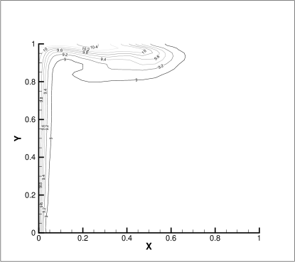
Figure 2: Isotemperature at time t=4.5s with algorithm 2. Distance to the critical point 1K.

3.2 The 2D Rayleigh Benard problem in a square cavity

In this second test case, we consider the Rayleigh-Benard [4, 7, 6] problem which consists in heating from bottom a square cavity filled with a supercritical fluid. The fluid is maintained at a constant temperature in the upper boundary of the cavity whereas the side boundaries are adiabatic and impermeable.

The square cavity is a two dimensional cavity with 10mm sides filled with CO${}_{\text{2}}$ on the critical isochore, initially at 1K above the critical temperature. A mesh of 70 x 90 is considered with strong refinement of the mesh at the four walls. The time step is kept constant at 0.05.

The results in this case agree well with those obtained by Amiroudine & al[4]. In figs 3 & 4, we show the temperature contours for an increase of 10mK of the bottom wall, for different times at 6.4s and 8.5s, respectively. We observe the thermal plumes which appear at the hot and cold walls. The piston effect generates a cold boundary layer at the top of the cavity where gravitational instabilities develop as well as at the heated bottom wall. In figure 5, we can see the corresponding velocity field at time 8.5s.

In this present case, we have the same speed up as for the side heated 2D cavity presented above but furthermore we can increase the time step by a factor of 10. which leads to a factor of 20 and more of CPU time gain.

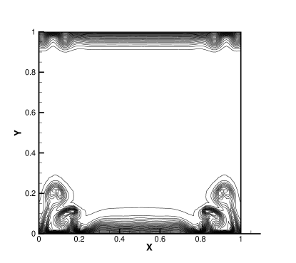
Figure 3: Isotemperature at time t=6.4s with algorithm 2. Distance to the critical point 1K. Same results as with algorithm 1 with a timestep 10 times bigger.

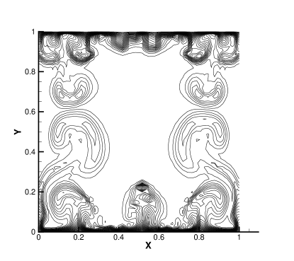
Figure 4: Isotemperature at time t=8.5s with algorithm 2. Distance to the critical point 1K.

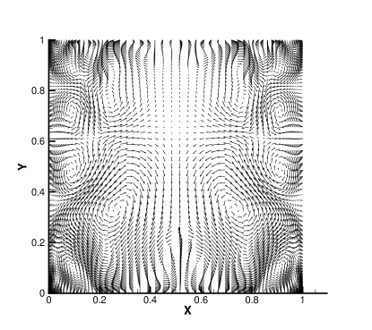
Figure 5: Velocity Field at time t=6s with algorithm 2. Distance to the critical point 1K.

4 Conclusion

In this paper, we have developed a new algorithm to solve low Mach number flows. The algorithm takes advantage of the low Mach number filtering by computing the divergence of velocity from the three combined equations (equation of state, mass conservation and energy), by doing so and using an Adams-Bashforth discretisation for the convective terms as well as for the viscous dissipation term, one can decouple at each time step the energy equation from the momentum and mass conservation equations. This decoupling results in a better stability of the full algorithm and allows for a substantial saving of CPU time. Even if time step limitations are introduced through the CFL condition, these limitations do not lower the time step as compared to the fully implicit case which is in fact limited in the time step size by physical aspects.

The other benefits of such an algorithm are to be able to use non iterative methods such as PISO, as well as other discretisation techniques such as pseudo spectral techniques, and it is easily applied to low mach number flows in general (as encountered in combustion problems). Existing code for ideal gas law can be easily modified to tackle supercritical fluids and 3D problems can be tackled in a reasonable amount of CPU times.

One other main reason to introduce such an algorithm for low Mach number critical fluids is to be able to treat problem with real equations of state other than van der Waals. These EOS are CPU time consuming and were not often used whereas now, we are introducing them in our 2D and 3D finite volume code.

References

- [1] Onuki A, Hao H, and Ferrell R A. Fast adiabatic equilibration in a single-component fluid near the liquid-vapor critical point. Phys Rev A 1990;41:2256-2257.
- [2] Zappoli B, Bailly D, Garrabos Y, Le Neindre B, Guenoun P, Beysens D. Anomalous heat transport by the piston effect in supercritical fluids under zero gravity. Phys Rev A 1990;41:2264-2267.
- [3] Zappoli B, Amiroudine S, Carlès P, Ouazzani J. Thermoacoustic and buoyancy-driven transport in a square side-heated cavity filled with a near critical-fluid. J Fluid Mech 1996;316:53-72.
- [4] Amiroudine S, Bontoux P, Larroudé P, Gilly B, Zappoli B. Direct numerical simulation of instabilities in a two dimensional near critical fluid layer heated from below. J. Fluid Mech 2001;442:119-40.
- [5] Accary G, Raspo I, Bontoux B, Zappoli B. An adaptation of the low Mach number approximation for supercritical fluid buoyant flows. C.R. Mecanique 2005;333:397-404.
- [6] Polezhaev V.I., Soboleva E.B. Rayleigh-Benard convection in a near-critical fluid in the neighborhood of the stability threshold. Fluid Dyn 2005;40(2):209-20.
- [7] Accary G, Raspo I. A 3D finite volume method for the prediction of a supercritical fluid buoyant flow in a differentially heated cavity. Comp Fluids 2006;35:1316-1331.
- [8] Guenoun P, Khalil B, Beysens D, Garrabos Y, Kammoun F, Le Neindre B, and Zappoli B. Thermal cycle around the critical point of carbon dioxide under reduced gravity. Phys. Rev. E 1993;47:1531-1540.
- [9] Garrabos Y, Bonetti M, Beysens D, Perrot F, Fröhlich T, Carlès P, and Zappoli B. Relaxation of a supercritical fluid after a heat pulse in the absence of gravity effects: Theory and experiments. Phys. Rev. E 1998;57:5665-5681.
- [10] Fröhlich T, Beysens D, and Garrabos Y. Piston-effect-induced thermal jets in near-critical fluids. Phys. Rev. E 2006;74:046307-13.
- [11] Paolucci S. On the filtering of sound from the Navier-Stokes equations. Technical report, Sandia National Laboratories USA, SAND82-8257, December 1982.
- [12] Muller B. Low-Mach number asymptotics of the Navier-Stokes equations. J Eng Math 1998;34(1-2):97-109.
- [13] Munz CD, Roller S, Klein R, Geratz KJ. The extension of incompressible flow solvers to the weakly compressible regime. Comp. Fluids 2003;32(2):173-96.
- [14] Patankar SV. Numerical heat transfer and fluid flow. New York:Hemisphere; 1980.
- [15] Oliveira PJ, Issa RI. An improved PISO algorithm for the computation of buoyancy-driven flows. Num. Heat Transfer B: Fund. (2001);40:473-493.
- [16] Peyret R, Taylor TD. Computational methods for fluid flow. Springer-Verlag, New York. 1983.
- [17] Guillard H, Viozat C. On the behaviour of upwind schemes in the low Mach number limit. Comp Fluids 1999;28:63-86.
- [18] Karki K, Patankar SV. Pressure based calculation procedure for viscous flows at all speed in arbitrary configurations. AIAA J 1989;27(9):1167-74.
- [19] Turkel E. Preconditioned methods for solving the incompressible and low speed compressible equations. J. Comput Phys 1987;72:277-98.
- [20] Choi YH, Merkle CL, The application of preconditioning in viscous flows. J. Comput. Phys. 1993;105(2):207-23.
- [21] Chorin AJ. A numerical method for solving the incompressible and low speed compressible equations. J Comput Phys 1997; 137(2):118-25.
- [22] Jounet A, Mojtabi A, Ouazzani J, Zappoli B., Low-frequency vibrations in a near critical fluid. Phys. Fluids. 2000;12(1);197-204.
- [23] Jounet A., Density relaxation of a near critical fluid in response to local heating and low frequency vibration in microgravity. Phys. Rev. E; 65:037301-1.
- [24] Ouazzani J, Zakaria A, Peyret R. Stability of collocation-Chebyshev schemes with application to the Navier-Stokes equations. Proc Num Meth Fluid Mech 1986 ;A87 :287-94.
- [25] Nicou F. Conservative High-Order finite difference schemes for low-Mach number flows. J. Comput. Phys. 2000;158:71-97.
- [26] Lessani B, Papalexandris MV. Time - accurate calculation of variable density flows with strong temperature gradients and combustion. J Comput Phys 2006;212:218-46.
- [27] Fröhlich J, Laure P, Peyret R. Large departures from Boussinesq approximations in the Rayleigh Benard problem. Phys Fluids A 1992;4(7):1335-72.