Stability Properties of Strongly Magnetized Spine Sheath Relativistic Jets

Abstract

The linearized relativistic magnetohydrodynamic (RMHD) equations describing a uniform axially magnetized cylindrical relativistic jet spine embedded in a uniform axially magnetized relativistically moving sheath are derived. The displacement current is retained in the equations so that effects associated with Alfvén wave propagation near light speed can be studied. A dispersion relation for the normal modes is obtained. Analytical solutions for the normal modes in the low and high frequency limits are found and a general stability condition is determined. A trans-Alfvénic and even a super-Alfénic relativistic jet spine can be stable to velocity shear driven Kelvin-Helmholtz modes. The resonance condition for maximum growth of the normal modes is obtained in the kinetically and magnetically dominated regimes. Numerical solution of the dispersion relation verifies the analytical solutions and is used to study the regime of high sound and Alfvén speeds.

1 Introduction

Relativistic jets are associated with active galactic nuclei and quasars (AGN), with black hole binary star systems (microquasars), and are thought responsible for the gamma-ray bursts (GRBs). In microquasar and AGN jets proper motions of intensity enhancements show mildly superluminal for the microquasar jets $\sim 1.2~{}c$ (Mirabel & Rodriquez 1999), range from subluminal ($\ll c$) to superluminal ($\lesssim 6~{}c$) along the M 87 jet (Biretta et al. 1995, 1999), are up to $\sim 25~{}c$ along the 3C 345 jet (Zensus et al. 1995; Steffen et al. 1995), and have inferred Lorentz factors $\gamma>100$ in the GRBs (e.g., Piran 2005). The observed proper motions along microquasar and AGN jets imply speeds from $\sim 0.9~{}c$ up to $\sim 0.999~{}c$, and the speeds inferred for the GRBs are $\sim 0.99999~{}c$.

Jets at the larger scales may be kinetically dominated and contain relatively weak magnetic fields, e.g., equipartition between magnetic and gas pressure or less, but the possibility of much stronger magnetic fields exists close to the acceleration and collimation region. Here general relativistic magnetohydrodynamic (GRMHD) simulations of jet formation (e.g., Koide et al. 2000; Nishikawa et al. 2005; De Villiers, Hawley & Krolik 2003; De Villiers et al. 2005; Hawley & Krolik 2006; McKinney 2006; Mizuno et al. 2006) and earlier theoretical work (e.g., Lovelace 1976; Blandford 1976; Blandford & Znajek 1977; Blandford & Payne 1982) invoke strong magnetic fields. In addition to strong magnetic fields, GRMHD simulation studies of jet formation indicate that highly collimated high speed jets driven by the magnetic fields threading the ergosphere may themselves reside within a broader wind or sheath outflow driven by the magnetic fields anchored in the accretion disk (e.g., McKinney 2006; Hawley & Krolik 2006; Mizuno et al. 2006). This configuration might additionally be surrounded by a less collimated accretion disk wind from the hot corona (e.g., Nishikawa et al. 2005).

That relativistic jets may have jet-wind structure is indicated by recent observations of high speed winds in several QSO’s with speeds, $\sim 0.1-0.4c$, (Chartas, Brandt & Gallagher 2002, Chartas et al. 2003; Pounds et al. 2003a; Pounds et al. 2003b; Reeves, O’Brien & Ward 2003). Other observational evidence such as limb brightening has been interpreted as evidence for a slower external sheath flow surrounding a faster jet spine, e.g., Mkn 501 (Giroletti et al. 2004), M 87 (Perlman et al. 2001), and a few other radio galaxy jets (e.g., Swain, Bridle & Baum 1998; Giovannini et al. 2001). Additional circumstantial evidence such as the requirement for large Lorentz factors suggested by the TeV BL Lacs when contrasted with much slower observed motions suggests the presence of a spine-sheath morphology (Ghisellini, Tavecchio & Chiaberge 2005). At hundreds of kiloparsec scales Siemignowska et al. (2007) have proposed a two component (spine-sheath) model to explain the broad-band emission from the PKS 1127-145 jet. A spine-sheath jet structure has been proposed based on theoretical arguments (e.g., Sol et al. 1989; Henri & Pelletier 1991; Laing 1996; Meier 2003). Similar type structure has been investigated in the context of GRB jets (e.g., Rossi, Lazzati & Rees 2002; Lazzatti & Begelman 2005; Zhang, Wooseley & MacFadyen 2003; Zhang, Woosley & Heger 2004; Morsony, Lazzati & Begelman 2006).

In order to study the effect of strong magnetic fields and the effect of a moving wind or sheath around a jet or jet spine, I begin by adopting a simple system with no radial dependence of quantities inside the jet spine and no radial dependence of quantities outside the jet in the sheath. This “top hat” configuration with magnetic fields parallel to the flow can be described exactly by the linearized relativistic magnetohydrodynamic (RMHD) equations. This system with no magnetic and flow helicity is stable to current driven (CD) modes of instability (Istomin & Pariev 1994, 1996; Lyubarskii 1999). However, this system can be unstable to Kelvin-Helmholtz (KH) modes of instability (Hardee 2004). This approach allows us to look at the potential KH modes without complications arising from coexisting CD modes (see Baty, Keppens & Compte 2004) and predictions can be verified by numerical simulations (Mizuno, Hardee & Nishikawa 2006).

This paper is organized as follows. In §2, I present the dispersion relation arising from a normal mode analysis of the linearized RMHD equations. Analytical approximate solutions to the dispersion relation for various limiting cases are given in §3. I verify the analytical solution through numerical solution of the dispersion relation in §4. I summarize the stability results in §5 and discuss the applicability of the present results in §6. Derivation of the linearized RMHD equations is shown in Appendix A, derivation of the normal mode dispersion relation is presented in Appendix B, and derivation of the analytical solutions is shown in Appendix C.

2 The RMHD Normal Mode Dispersion Relation

Let us analyze the stability of a spine-sheath system by modeling the jet spine as a cylinder of radius R, having a uniform proper density, $\rho_{j}$, a uniform axial magnetic field, $B_{j}=B_{j,z}$, and a uniform velocity, $\mathbf{u}_{j}=u_{j,z}$. The external sheath is assumed to have a uniform proper density, $\rho_{e}$, a uniform axial magnetic field, $B_{e}=B_{e,z}$, a uniform velocity $\mathbf{u}_{e}=u_{e,z}$, and extends to infinity. The sheath velocity corresponds to an outflow around the central spine if $u_{e,z}>0$ or represents backflow when $u_{e,z}<0$. The jet spine is established in static total pressure balance with the external sheath where the total static uniform pressure is $P_{e}^{\ast}\equiv P_{e}+B_{e}^{2}/8\pi=P_{j}^{\ast}\equiv P_{j}+B_{j}^{2}/8\pi$, and the initial equilibrium satisfies the zeroth order equations. Formally, the assumption of an infinite sheath means that a dispersion relation could be derived in the reference frame of the sheath with results transformed to the source/observer reference frame. However, it is not much more difficult to derive a dispersion relation in the source/observer frame in which analytical solutions to the dispersion relation take on simple revealing forms. Additionally, this approach lends itself to modeling the propagation and appearance of jet structures viewed in the source/observer frame, e.g., helical structures in the 3C 120 jet (Hardee, Walker & Gómez 2005).

The general approach to analyzing the time dependent properties of this system is to linearize the ideal RMHD and Maxwell equations, where the density, velocity, pressure and magnetic field are written as $\rho=\rho_{0}+\rho_{1}$, $\mathbf{v}=\mathbf{u}+\mathbf{v}_{1}$ (we use $\mathbf{v}_{0}\equiv\mathbf{u}$ for notational reasons), $P=P_{0}+P_{1}$, and $\mathbf{B}=\mathbf{B}_{0}+\mathbf{B}_{1}$, where subscript 1 refers to a perturbation to the equilibrium quantity with subscript 0. Additionally, the Lorentz factor $\gamma^{2}=(\gamma_{0}+\gamma_{1})^{2}\simeq\gamma_{0}^{2}+2\gamma_{0}^{4}\mathbf{u\cdot v}_{1}/c^{2}$ where $\gamma_{1}=\gamma_{0}^{3}\mathbf{u\cdot v}_{1}/c^{2}$. The linearization is shown in Appendix A. In cylindrical geometry a random perturbation $\rho_{1}$, $\mathbf{v}_{1}$ $\mathbf{B}_{1}$ and $P_{1}$ can be considered to consist of Fourier components of the form

$$f_{1}(r,\phi,z,t)=f_{1}(r)\exp[i(kz\pm n\phi-\omega t)]$$ (1)

where flow is along the z-axis, and r is in the radial direction with the flow bounded by $r=R$. In cylindrical geometry $n$ is an integer azimuthal wavenumber, for $n>0$ waves propagate at an angle to the flow direction, and $+n$ and $-n$ give wave propagation in the clockwise and counter-clockwise sense, respectively, when viewed in the flow direction. In equation (1) $n=0$, $1$, $2$, $3$, $4$, etc. correspond to pinching, helical, elliptical, triangular, rectangular, etc. normal mode distortions of the jet, respectively. Propagation and growth or damping of the Fourier components can be described by a dispersion relation of the form

$$\frac{\beta_{j}}{\chi_{j}}\frac{J_{n}^{{}^{\prime}}(\beta_{j}R)}{J_{n}(\beta_{j}R)}=\frac{\beta_{e}}{\chi_{e}}\frac{H_{n}^{(1)^{\prime}}(\beta_{e}R)}{H_{n}^{(1)}(\beta_{e}R)}~{}.$$ (2)

Derivation of this dispersion relation is given in Appendix B. In the dispersion relation $J_{n}$ and $H_{n}^{(1)}$ are Bessel and Hankel functions, the primes denote derivatives of the Bessel and Hankel functions with respect to their arguments. In equation (2)

$$\chi_{j}\equiv\gamma_{j}^{2}\gamma_{Aj}^{2}W_{j}\left(\varpi_{j}^{2}-\kappa_{j}^{2}v_{Aj}^{2}\right)~{},$$ ()

$$\chi_{e}\equiv\gamma_{e}^{2}\gamma_{Ae}^{2}W_{e}\left(\varpi_{e}^{2}-\kappa_{e}^{2}v_{Ae}^{2}\right)~{},$$ ()

and

$$\beta_{j}^{2}\equiv\left[\frac{\gamma_{j}^{2}\left(\varpi_{j}^{2}-\kappa_{j}^{2}a_{j}^{2}\right)\left(\varpi_{j}^{2}-\kappa_{j}^{2}v_{Aj}^{2}\right)}{v_{msj}^{2}\varpi_{j}^{2}-\kappa_{j}^{2}v_{Aj}^{2}a_{j}^{2}}\right]~{},$$ ()

$$\beta_{e}^{2}\equiv\left[\frac{\gamma_{e}^{2}\left(\varpi_{ex}^{2}-\kappa_{e}^{2}a_{e}^{2}\right)\left(\varpi_{e}^{2}-\kappa_{e}^{2}v_{Ae}^{2}\right)}{v_{mse}^{2}\varpi_{e}^{2}-\kappa_{e}^{2}v_{Ae}^{2}a_{e}^{2}}\right]~{}.$$ ()

In equations (3a & 3b) and equations (4a & 4b) $\varpi_{j,e}^{2}\equiv\left(\omega-ku_{j,e}\right)^{2}$ and $\kappa_{j,e}^{2}\equiv\left(k-\omega u_{j,e}/c^{2}\right)^{2}$, $\gamma_{j,e}\equiv(1-u_{j,e}^{2}/c^{2})^{-1/2}$ is the flow Lorentz factor, $\gamma_{Aj,e}\equiv(1-v_{Aj,e}^{2}/c^{2})^{-1/2}$ is the Alfvén Lorentz factor, $W\equiv\rho+\left[\Gamma/\left(\Gamma-1\right)\right]P/c^{2}$ is the enthalpy, $a$ is the sound speed, $v_{A}$ is the Alfvén wave speed, and $v_{ms}$ is a magnetosonic speed. The sound speed is defined by

$$a\equiv\left[\frac{\Gamma P}{\rho+\left(\frac{\Gamma}{\Gamma-1}\right)P/c^{2}}\right]^{1/2}~{},$$

where $4/3\leq\Gamma\leq 5/3$ is the adiabatic index. The Alfvén wave speed is defined by

$$v_{A}\equiv\left[\frac{V_{A}^{2}}{1+V_{A}^{2}/c^{2}}\right]^{1/2}$$

where $V_{A}^{2}\equiv B_{0}^{2}/(4\pi W_{0})$. A magnetosonic speed corresponding to the fast magnetosonic speed for propagation perpendicular to the magnetic field (e.g., Vlahakis & Königl 2003) is defined by

$$v_{ms}\equiv\left[a^{2}+v_{A}^{2}-a^{2}v_{A}^{2}/c^{2}\right]^{1/2}=\left[a^{2}/\gamma_{A}^{2}+v_{A}^{2}\right]^{1/2}~{}.$$

3 Analytical Solutions to the Dispersion Relation

In this section analytical solutions to the dispersion relation in the low frequency limit, in the fluid and magnetic limits at resonance (maximum growth), and in the high frequency limit are summarized. The analytical solutions are derived in Appendix C.

3.1 Low Frequency Limit

Analytically each normal mode $n$ contains a single fundamental/surface wave ($\omega\longrightarrow 0$, $k\longrightarrow 0$, $\omega/k>0$) solution and multiple body wave ($\omega\longrightarrow 0$, $k>0$, $\omega/k\longrightarrow 0$) solutions that satisfy the dispersion relation. In the low frequency limit the fundamental pinch mode ($n=0$) solution is given by

$$\frac{\omega}{k}=\frac{u_{j}\pm v_{w}}{1\pm v_{w}u_{j}/c^{2}}$$ (5)

where the pinch fundamental mode wave speed

$$v_{w}^{2}\approx a_{j}^{2}\left\{\frac{v_{Aj}^{2}}{v_{msj}^{2}}+\delta\left[\frac{v_{Aj}^{2}}{v_{msj}^{2}}-1\right]\right\}~{},$$ (6)

and

$$\delta\equiv-\frac{1}{2}\gamma_{e}^{2}\frac{\gamma_{Ae}^{2}}{\gamma_{Aj}^{2}}\frac{W_{e}}{W_{j}}\frac{\left(\varpi_{e}^{2}-\kappa_{e}^{2}v_{Ae}^{2}\right)}{v_{msj}^{2}}R^{2}\left[\ln(\frac{\beta_{e}R}{2})+\frac{\pi}{2}\epsilon-i\frac{\pi}{2}\right]$$ (7)

with $\left|\delta\right|\propto\left|k^{2}R^{2}\right|<<1$.  In this limit $\delta$ is complex and this mode consists of a growing and damped wave pair. The imaginary part of the solution is vanishingly small in the low frequency limit. The above form indicates that growth, which arises from the complex value of $\delta$, will be reduced as $(v_{Aj}^{2}/v_{msj}^{2})\longrightarrow 1$. The unstable growing solution is associated with the backwards moving (in the jet fluid reference frame) wave.

In the low frequency limit the surface helical, elliptical, and higher order normal modes ($n>0$) have a solution given by

$$\frac{\omega}{k}=\frac{\left[\eta u_{j}+u_{e}\right]\pm i\eta^{1/2}\left[\left(u_{j}-u_{e}\right)^{2}-V_{As}^{2}/\gamma_{j}^{2}\gamma_{e}^{2}\right]^{1/2}}{(1+V_{Ae}^{2}/\gamma_{e}^{2}c^{2})+\eta(1+V_{Aj}^{2}/\gamma_{j}^{2}c^{2})}$$ (8)

where $\eta\equiv\gamma_{j}^{2}W_{j}\left/\gamma_{e}^{2}W_{e}\right.$ and a “surface” Alfvén speed is defined by

$$V_{As}^{2}\equiv\left(\gamma_{Aj}^{2}W_{j}+\gamma_{Ae}^{2}W_{e}\right)\frac{B_{j}^{2}+B_{e}^{2}}{4\pi W_{j}W_{e}}~{}.$$ (9)

In equation (9) note that the Alfvén Lorentz factor $\gamma_{Aj,e}^{2}=1+V_{Aj,e}^{2}/c^{2}$. Thus, the jet is stable to $n>0$ surface wave mode perturbations when

$$\gamma_{j}^{2}\gamma_{e}^{2}\left(u_{j}-u_{e}\right)^{2}<\gamma_{Aj}^{2}\gamma_{Ae}^{2}\left(W_{j}/\gamma_{Ae}^{2}+W_{e}/\gamma_{Aj}^{2}\right)\frac{B_{j}^{2}+B_{e}^{2}}{4\pi W_{j}W_{e}}~{}.$$ (10)

For example, with $u_{j}\approx c>>u_{e}$, $\gamma_{e}^{2}\approx 1$, $\gamma_{Aj}^{2}>>\gamma_{Ae}^{2}\approx 1$, $B_{j}^{2}>>B_{e}^{2}$, and using $\gamma_{Aj}^{2}=1+B_{j}^{2}/4\pi W_{j}c^{2}$ the jet is stable when

$$\gamma_{j}^{2}<\left[1+\frac{B_{j}^{2}}{4\pi W_{e}c^{2}}\right]\gamma_{Aj}^{2}$$ ()

or with $B_{e}=B_{j}$, $W_{e}=W_{j}$, so that $v_{A,j}=v_{A,e}$, and with $\gamma_{A}\equiv\gamma_{A,e}=\gamma_{A,j}$ the jet is stable when

$$\gamma_{j}^{2}\gamma_{e}^{2}(u_{j}-u_{e})^{2}<4\gamma_{A}^{2}(\gamma_{A}^{2}-1)c^{2}~{}.$$ ()

Thus, the jet can remain stable to the surface wave modes even when the jet Lorentz factor exceeds the Alfvén Lorentz factor.

In the low frequency limit the real part of the body wave solutions is given by

$$kR\approx k_{nm}^{\min}R\equiv\left[\frac{v_{msj}^{2}u_{j}^{2}-v_{Aj}^{2}a_{j}^{2}}{\gamma_{j}^{2}(u_{j}^{2}-a_{j}^{2})(u_{j}^{2}-v_{Aj}^{2})}\right]^{1/2}\times\left[(n+2m-1/2)\pi/2+(-1)^{m}\epsilon_{n}\right]$$ (12)

where $n$ specifies the normal mode, $m=1,2,3,...$ specify the first, second, third, etc. body wave solutions, and

$$\epsilon_{n}\equiv\frac{\chi_{e}}{\chi_{j}}\frac{\beta_{e}}{\beta_{j}}\left(\frac{\pi\beta_{j}R}{2}\right)^{1/2}J_{n}^{{}^{\prime}}(\beta_{j}R)\frac{H_{n}^{(1)}(\beta_{e}R)}{H_{n}^{(1)^{\prime}}(\beta_{e}R)}~{}.$$

In the absence of a significant external magnetic field and a significant external flow $\epsilon_{n}=0$ as $\chi_{e}=\gamma_{e}^{2}\gamma_{Ae}^{2}W_{e}\left[u_{e}^{2}-v_{Ae}^{2}\right]k^{2}=0$. In this low frequency limit the body wave solutions are either purely real or damped, exist only when $k_{nm}^{\min}R$ has a positive real part, and with $\left|\epsilon_{n}\right|<<1$ require that

$$\left[\frac{v_{msj}^{2}u_{j}^{2}-v_{Aj}^{2}a_{j}^{2}}{\gamma_{j}^{2}(u_{j}^{2}-a_{j}^{2})(u_{j}^{2}-v_{Aj}^{2})}\right]>0~{}.$$ (13)

Thus, the body modes can exist when the jet is supersonic and super-Alfvénic, i.e., $u_{j}^{2}-a_{j}^{2}>0$ and $u_{j}^{2}-v_{Aj}^{2}>0$, or in a limited velocity range given approximately by $a_{j}^{2}>u_{j}^{2}>[\gamma_{sj}^{2}/(1+\gamma_{sj}^{2})]a_{j}^{2}$ when $v_{Aj}^{2}\approx a_{j}^{2}$, where $\gamma_{sj}\equiv(1-a_{j}^{2}/c^{2})^{-1/2}$ is a sonic Lorentz factor.

3.2 Resonance

With the exception of the pinch fundamental mode which can have a relatively broad plateau in the growth rate, all body modes, and all surface modes can have a distinct maximum in the growth rate at some resonant frequency.

The resonance condition can be evaluated analytically in either the fluid limit where $a>>V_{A}$ or in the magnetic limit where $V_{A}>>a$. Note that in the magnetic limit, magnetic pressure balance implies that $B_{j}=B_{e}$. In these cases a necesary condition for resonance is that

$$\frac{u_{j}-u_{e}}{1-u_{j}u_{e}/c^{2}}>\frac{v_{wj}+v_{we}}{1+v_{wj}v_{we}/c^{2}}~{},$$ (14)

where $v_{wj}\equiv\left(a_{j},v_{Aj}\right)$ and $v_{we}\equiv\left(a_{e},v_{Ae}\right)$ in the fluid or magnetic limits, respectively. When this condition is satisfied it can be shown that the wave speed at resonance is

$$v_{w}\approx v_{w}^{\ast}\equiv\frac{\gamma_{j}(\gamma_{we}v_{we})u_{j}+\gamma_{e}(\gamma_{wj}v_{wj})u_{e}}{\gamma_{j}(\gamma_{we}v_{we})+\gamma_{e}(\gamma_{wj}v_{wj})}$$ (15)

where $\gamma_{w}\equiv(1-v_{w}^{2}/c^{2})^{-1/2}$ is the sonic or Alfvénic Lorentz factor accompanying $v_{wj}\equiv\left(a_{j},v_{Aj}\right)$ and $v_{we}\equiv\left(a_{e},v_{Ae}\right)$ in the fluid or magnetic limits, respectively.

The resonant wave speed and maximum growth rate occur at a frequency given by

$$\omega R/v_{we}\approx\omega_{nm}^{\ast}R/v_{we}\equiv\frac{(2n+1)\pi/4+m\pi}{\left[\left(1-u_{e}/v^{\ast}_{w}\right)^{2}-\left(v_{we}/v^{\ast}_{w}-u_{e}v_{we}/c^{2}\right)^{2}\right]^{1/2}}~{}.$$ (16)

In equation (16) $n$ specifies the normal mode, $m=0$ specifies the surface wave, and $m\geq 1$ specifies the body waves. In the limit of insignificant sheath flow, $u_{e}=0$, and using eq. (15) for $v_{w}^{\ast}$ in eq. (16) allows the resonant frequency to be written as

$$\omega_{nm}^{\ast}R_{j}/v_{we}=\frac{(2n+1)\pi/4+m\pi}{\left[1-\left(v_{we}^{2}/u_{j}^{2}+2\frac{\gamma_{wj}}{\gamma_{we}}v_{we}v_{wj}/\gamma_{j}u_{j}^{2}+\frac{\gamma_{wj}^{2}}{\gamma_{we}^{2}}v_{wj}^{2}/\gamma_{j}^{2}u_{j}^{2}\right)\right]^{1/2}}~{},$$

and this predicts a resonant frequency that is primarily a function of the sound and Alfvén wave speeds in the sheath. The effect of sheath flow is best illustrated by assuming comparable conditions in the spine and sheath, $\gamma_{wj}v_{wj}\sim\gamma_{we}v_{we}$, and assuming that $\gamma_{j}u_{j}>>\gamma_{e}u_{e}$ in which case

$$\omega_{nm}^{\ast}R_{j}/v_{we}\sim\frac{(2n+1)\pi/4+m\pi}{\gamma_{e}\left[1-2\left(u_{e}/u_{j}\right)(1-v_{we}^{2}/c^{2})-\left(v_{we}^{2}-u_{e}^{2}\right)/u_{j}^{2}\right]^{1/2}}~{}.$$

The term $u_{e}/u_{j}$ in the denominator indicates that the resonant frequency increases as the shear speed, $u_{j}-u_{e}$, declines. In the limit

$$\frac{u_{j}-u_{e}}{1-u_{j}u_{e}/c^{2}}\longrightarrow\frac{v_{wj}+v_{we}}{1+v_{wj}v_{we}/c^{2}}~{},$$

the resonant frequency $\omega_{nm}^{\ast}R/v_{we}\longrightarrow\infty$.

The resonant wavelength is given by $\lambda\approx\lambda_{nm}^{\ast}\equiv 2\pi v_{w}^{\ast}/\omega_{nm}^{\ast}$ and can be calculated from

$$\lambda_{nm}^{\ast}\equiv\frac{2\pi}{(2n+1)\pi/4+m\pi}\left(\frac{\gamma_{e}}{v_{we}}\right)\left\{\left(v_{w}^{\ast}-u_{e}\right)^{2}-\left[v_{we}-(v_{we}u_{e}/c^{2})v_{w}^{\ast}\right]^{2}\right\}^{1/2}R~{}.$$ (17)

Equations (15 - 17) provide the proper functional dependence of the resonant wave speed, frequency and wavelength provided $(u_{e}/u_{j})^{2}<<1$ and $(v_{we}/u_{j})^{2}<<1$.

With the exception of the $n=0$, $m=0$, fundamental pinch mode, a maximum spatial growth rate, $k_{I}^{\rm max}$, is approximated by

$$k_{I}^{\rm max}R\approx k_{I}^{\ast}R\equiv-\frac{1}{2}\frac{v_{wj}}{\gamma_{j}u_{j}}\ln\left|\mathcal{R}\right|~{},$$ (18)

where

$$\left|\mathcal{R}\right|\approx\left[\frac{4\left(\omega_{nm}^{\ast}R/v_{we}\right)^{2}\left(1-2u_{e}/u_{j}\right)+\left(\ln\left|\mathcal{R}\right|/2\right)^{2}}{\left(\ln\left|\mathcal{R}\right|/2\right)^{2}}\right]^{1/2}~{}.$$ (19)

Equations (18) and (19) show that the maximum growth rate is primarily a function of the jet sound, Alfvén and flow speed through $v_{wj}/\gamma_{j}u_{j}$, and secondarily a function of the sheath sound, Alfvén and flow speed through $\left(\omega_{nm}^{\ast}R/v_{we}\right)^{2}\left(1-2u_{e}/u_{j}\right)$.

I can illustrate the dependencies of the maximum growth rate on sound, Alfvén and flow speeds by using

$$\left(\frac{\omega_{nm}^{\ast}R}{v_{we}}\right)^{2}\left(1-2u_{e}/u_{j}\right)\approx\frac{\left(1-2u_{e}/u_{j}\right)}{\left[1-2\left(u_{e}/u_{j}\right)(1-v_{we}^{2}/c^{2})-(v_{we}^{2}-u_{e}^{2})/u_{j}^{2}\right]}\times\left[(2n+1)\pi/4+m\pi\right]^{2}$$

and if say $u_{e}=0$, then

$$\left(\left|\mathcal{R}\right|^{2}-1\right)^{1/2}\ln\left|\mathcal{R}\right|\approx 4\left[\frac{1}{1-v_{we}^{2}/u_{j}^{2}}\right]^{1/2}\times\left[(2n+1)\pi/4+m\pi\right]~{}.$$ (20)

Thus, $\left|\mathcal{R}\right|$ increases as $\omega_{nm}^{\ast}$ increases for higher order modes with larger $n$ and larger $m$ and this result indicates an increase in the growth rate for larger $n$ and larger $m$. When the sound or Alfvén wave speed, $v_{we}$, increases $\left|\mathcal{R}\right|$ increases. This result indicates an increase in the growth rate at the higher resonant frequency accompanying an increase in the sound or Alfvén wave speed in the sheath.

The behavior of the maximum growth rate as the shear speed, $u_{j}-u_{e}$, declines is best illustrated by considering the effect of an increasing wind speed where $(v_{we}^{2}-u_{e}^{2})/u_{j}^{2}<<1$ is ignored. In this case

$$\left(\left|\mathcal{R}\right|^{2}-1\right)^{1/2}\ln\left|\mathcal{R}\right|\approx 4\left[(2n+1)\pi/4+m\pi\right]$$ (21)

and $\left|\mathcal{R}\right|$ will remain relatively independent of $\omega_{nm}^{\ast}$ even as $\omega_{nm}^{\ast}\longrightarrow\infty$ as the shear speed decreases. This result indicates a relatively constant resonant growth rate as the shear speed decreases.

In the fluid limit decline in the shear speed ultimately results in a decrease in the growth rate and increase in the spatial growth length. This decline in the growth rate is also indicated by equation (8) which, in the fluid limit, becomes

$$\frac{\omega}{k}=\frac{\eta u_{j}+u_{e}}{1+\eta}\pm i\frac{\eta^{1/2}}{1+\eta}\left(u_{j}-u_{e}\right)~{}.$$ (22)

Equation (22) applies to frequencies below the resonant frequency $\omega_{nm}^{\ast}$ and directly reveals the decline in growth rates as $u_{j}-u_{e}\longrightarrow 0$.

In the magnetic limit the resonant frequency $\omega_{nm}^{\ast}R/v_{Ae}\longrightarrow\infty$ as

$$\frac{u_{j}-u_{e}}{1-u_{j}u_{e}/c^{2}}\longrightarrow\frac{v_{Aj}+v_{Ae}}{1+v_{Aj}v_{Ae}/c^{2}}~{}.$$ (23)

Here equation (8) indicates that the jet is stable when

$$\gamma_{j}^{2}\gamma_{e}^{2}\left(u_{j}-u_{e}\right)^{2}<V_{As}^{2}~{},$$

and the jet will be stable as $\omega_{nm}^{\ast}\longrightarrow\infty$ when

$$\gamma_{j}^{2}\gamma_{e}^{2}\left(1-u_{j}u_{e}/c^{2}\right)^{2}<2\gamma_{Aj}^{2}\gamma_{Ae}^{2}\frac{v_{Ae}^{2}+v_{Aj}^{2}}{\left(v_{Aj}+v_{Ae}\right)^{2}}\left(1+v_{Aj}v_{Ae}/c^{2}\right)^{2}~{},$$ (24)

where I have used an equality in equation (23) in equation (8) to obtain equation (24). Equation (24) indicates that a high jet speed relative to the Alfvén wave speed is necessary for instability. For example, if $v_{A}\equiv v_{Aj}=v_{Ae}$ and $u_{e}=0$, the jet is stable at high frequencies provided

$$\gamma_{j}^{2}<\left(1+v_{A}^{2}/c^{2}\right)^{2}\gamma_{A}^{4}~{}.$$ ()

This high frequency condition is slightly different from the low frequency stabilization condition found when $v_{A}\equiv v_{Aj}=v_{Ae}$ and $u_{e}=0$ from equation (11b)

$$\gamma_{j}^{2}(u_{j}/c)^{2}<4\gamma_{A}^{2}(\gamma_{A}^{2}-1)~{}.$$ ()

Note that eqs. (25a & 25b) are identical in the large Lorentz factor limit. Equations (25) predict that stabilization at high frequencies occurs at somewhat higher jet speeds than stabilization at lower frequencies. Determination of stabilization at intermediate frequencies requires numerical solution of the dispersion relation. A non-negligable postive external flow requires even higher jet speeds for the jet to be unstable. Thus, a strongly magnetized relativistic trans-Alfvénic jet is predicted to be KH stable and a super-Alfvénic jet can be KH stable.

3.3 High Frequency Limit

Provided the condition, eq. (14), for resonance is met, the real part of the solutions to the dispersion relation in the high frequency limit for fundamental, surface, and body modes is given by

$$\frac{\omega}{k}\approx\frac{u_{j}\pm v_{wj}}{1\pm v_{wj}u_{j}/c^{2}}~{}.$$ (26)

and describes sound waves $v_{wj}=a_{j}$ or Alfvén waves $v_{wj}=v_{Aj}$ propagating with and against the jet flow inside the jet. Unstable growing solutions are associated with the backwards moving (in the jet fluid reference frame) wave but the growth rate is vanishingly small in this limit.

4 Numerical Solution of the Dispersion Relation

The detailed behavior of solutions within an order of magnitude of the resonant frequency and for comparable sound and Alfvén wave speeds must be investigated by numerical solution of the dispersion relation. Analytical solutions found in the previous section can be used for initial estimates and to provide the functional behavior of solutions. Numerical solution of the dispersion relation also allows a determination of the accuracy and applicability of the analytical expressions in §3.

In this section pinch fundamental, helical surface and elliptical surface, and the associated first body modes are investigated in the fluid, magnetic and magnetosonic regimes. These modes are chosen as they have been identified with structure seen in relativistic hydrodynamic (RHD) numerical simulations or tentatively identified with structures in resolved AGN jets. For example, trailing shocks in a numerical simulation (Agudo et al. 2002) and in the 3C 120 jet (Gómez et al. 2001) have been identified with the first pinch body mode. The development of large scale helical twisting of jets has been attributed to or may be associated with growth of the helical surface mode, e.g., 3C 449 (Hardee 1981) and Cygnus A (Hardee 1996) Additionally, the development of twisted filamentary structures has been attributed to helical and elliptical surface and first body modes, e.g., 3C 273 (Lobanov & Zensus 2001), M 87 (Lobanov, Hardee & Eilek 2003), 3C 120 (Hardee, Walker & Gómez 2005), and have been studied in RHD numerical simulations, e.g., Hardee & Hughes (2003); Perucho et al. (2006).

4.1 Fluid Limit

In this section the basic behavior of the pinch (F) fundamental, helical (S) surface and elliptical (S) surface modes is investigated: (1) as a function of varying sound speed in the external sheath or jet spine for a fixed sound speed in the jet spine or external sheath and no sheath flow, (2) as a function of equal sound speeds in the jet spine and external sheath for no sheath flow, and (3) as a function of sheath flow for a relatively high sound speed equal in jet spine and external sheath. In general only growing solutions are shown and complexities associated with multiple crossing solutions are not shown. For all solutions shown the jet spine Lorentz factor and speed are set to $\gamma=2.5$ and $u_{j}=0.9165~{}c$. Sound speeds are input directly with the only constant being the sheath number density. Total pressure and spine density are quantities computed for the specified sound speeds. The adiabatic index is chosen to be $\Gamma=13/9$ when $0.1\leq a_{j,e}/c\leq 0.5$ consistent with relativistically hot electrons and cold protons (Synge 1957). For sound speeds $a_{j,e}\sim c/\sqrt{3}$ the adiabatic index is set to $\Gamma=4/3$. Solutions shown assume zero magnetic field. Test calculations with magnetic fields giving magnetic pressures a few percent of the gas pressure and Alfvén wave speeds an order of magnitude less than the sound speeds give almost identical results.

In Figure 1 solutions in the left column are for a fixed jet spine sound speed $a_{j}=0.3~{}c$ and in the right column are for a fixed external sheath sound speed $a_{e}=0.3~{}c$. The solutions shown in Figure 1 confirm the accuracy of the low frequency solutions to the pinch fundamental mode, eqs. (5 & 6), and the helical and elliptical surface modes, eq. (8). Note that fast or slow wave speeds are possible at low frequencies depending on whether $\eta\simeq(\gamma_{j}a_{e}/\gamma_{e}a_{j})^{2}$ in eq. (8) is much greater or much less than one, respectively. The numerical solutions to the dispersion relation show that the maximum growth rate is primarily a function of the jet spine sound speed and only secondarily a function of the external sheath sound speed as indicated by eqs. (18 - 20). Where a distinct supersonic resonance exists, the resonant frequency is primarily a function of the external sheath sound speed as predicted from eq. (16). The analytical expression for the resonant frequency for the helical and elliptical surface modes provides the correct functional variation to within a constant multiplier provided $a_{e}\leq c/\sqrt{3}$ and $a_{j}<c/3$. A dramatic increase in the resonant frequency and modest increase in the growth rate for larger jet spine sound speeds indicates the transition to transonic behavior. Equation (15) for the resonant wave speed and equation (17) for the resonant wavelength also provide a reasonable approximation to the functional variations provided $a_{e}\leq c/\sqrt{3}$ and $a_{j}<c/3$. These results confirm the resonant solutions found in §3.2. At frequencies more than an order of magnitude above resonance the growth rate is greatly reduced and solutions approach the high frequency limiting form given by eq. (26). Note that eq. (26) allows only relatively high wave speeds at high frequencies because $a_{j}\leq c/\sqrt{3}$.

In Figure 2 the behavior of solutions to the fundamental/surface (left column) and associated first body mode (right column) shows how solutions change as the sound speed increases in both the jet spine and external sheath. Here I illustrate the transition from supersonic to transonic behavior for no flow in the sheath. At low frequencies the modes behave as predicted by the analytic solutions given in §3.1. The solutions show the expected shift to a higher resonant frequency that is primarily a function of the increased external sheath sound speed and an accompanying increase in the resonant growth rate that is primarily a function of the increased jet spine sound speed. The resonance disappears as sound speeds approach $c/\sqrt{3}$ as the jet becomes transonic as predicted by the resonance condition in §3.2.

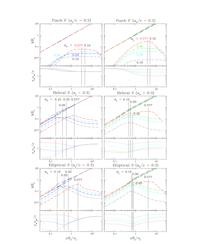
Figure 1: Solutions to the dispersion relation for pinch fundamental, helical surface and elliptical surface modes for different sound speeds in the sheath (left column) and in the spine (right column) are shown for no sheath flow. The real part of the wavenumber, $k_{r}R_{j}$, is shown by the dashed lines and the imaginary part , $k_{i}R_{j}$, is shown by the dash-dot lines as a function of the dimensionless angular frequency, $\omega R_{j}/u_{j}$. For the pinch mode the vertical lines indicate the maximum growth rate range. Otherwise, the vertical lines indicate the location of maximum growth. Immediately under the dispersion relation solution panel is a panel that shows the relativistic wave speed, $\gamma_{w}v_{w}/c$. Line colors indicate the sound speed in units of c: (black) 0.10, (blue) 0.20, (cyan) 0.30, (green) 0.40, & (red) 0.577.

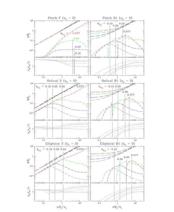
Figure 2: Solutions to the dispersion relation for pinch fundamental, helical surface, elliptical surface (left column) and the first body (right column) modes are shown for equal sound speeds in spine and sheath and no sheath flow. Real and imaginary parts of the wavenumber as a function of angular frequency are shown as in Figure 1. Locations of the maximum growth rate are indicated by the vertical solid lines. A vertical arrow (helical B1) indicates a narrow damping feature. The underlying panel shows the relativistic wave speed, $\gamma_{w}v_{w}/c$. Line colors indicate the sound speed in units of c: (black) 0.10, (blue) 0.20, (green) 0.40, & (red) 0.577.

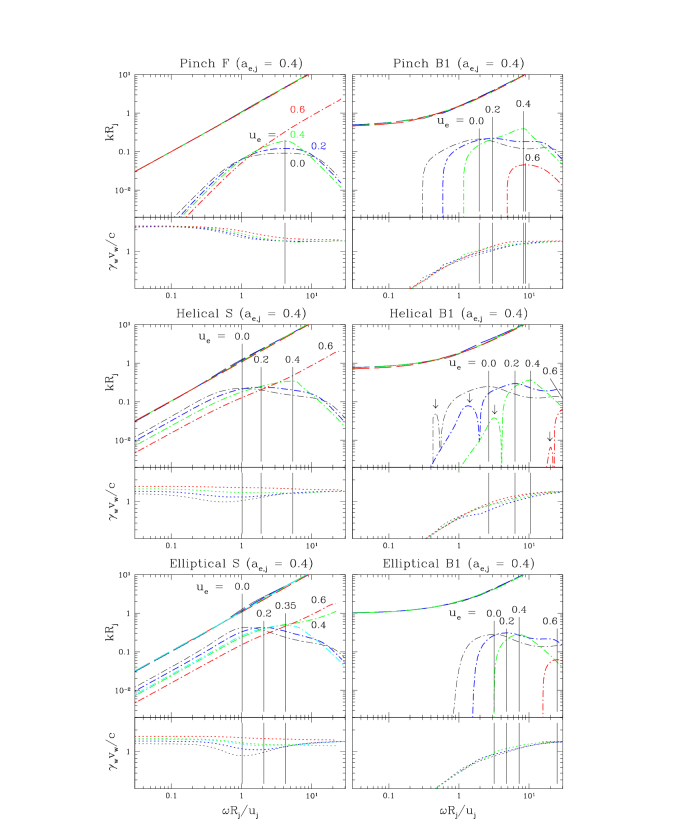
Figure 3: Solutions to the dispersion relation for pinch fundamental, helical surface, elliptical surface (left column) and first body (right column) modes as a function of the sheath speed for equal sound speeds in spine and sheath. Real and imaginary parts of the wavenumber as a function of angular frequency are shown as in Figure 1. Locations of the maximum growth rate are indicated by the vertical solid lines. Vertical arrows (helical B1) indicate damping features. The underlying panel shows the relativistic wave speed, $\gamma_{w}v_{w}/c$. Line colors indicate the sheath speed in units of c: (black) 0.0, (blue) 0.20, (cyan) 0.35, (green) 0.40, & (red) 0.60.

In the transonic regime high frequency fundamental/surface mode growth rates and wave speeds are identical with wave speeds given by eq. (26). Provided the jet is sufficiently supersonic, i.e., $a_{j,e}<0.5~{}c$, the maximum growth rate of the first body mode is greater than that of the pinch fundamental mode, is comparable to that of the helical surface mode, and is less than that of the elliptical surface mode. A narrow damping peak shown for the helical first body (B1) solution when $a_{j,e}=0.4~{}c$ is indicative of complexities in the body mode solution structure. In the transonic regime growth of the first body mode is less than that of the pinch fundamental, helical surface and elliptical surface modes.

Figure 3 illustrates the behavior of fundamental/surface and first body modes as a function of the sheath speed for equal sound speeds in spine and sheath of $a_{j,e}=0.4~{}c$. For this value of the sound speeds a sheath speed $u_{e}=0$ provides a supersonic solution structure baseline. At low frequencies the surface modes behave as predicted by eq. (8), and the wave speed rises as $u_{e}$ increases. As $u_{e}$ increases the resonant frequency increases in accordance with eq. (16). On the other hand, the growth rate at resonance does not vary significantly in accordance with eqs. (18 & 19). When the sheath speed exceeds the sound speed, solutions make a transition from supersonic to transonic structure. Note that the transition point between supersonic and transonic behavior is similar but not identical for the helical and elliptical surface modes, i.e., ocurs at a slightly lower sheath speed for the elliptical mode. The first body modes also show an increase in resonant frequency with little change in the maximum growth rate provided the sheath speed remains below the sound speed. A significant damping feature in the helical first body (B1) panel, is found. While a similar damping feature was not found for the pinch and elliptical first body mode, this does not indicate a significant difference as the root finding technique does not find all structure associated with the body modes. The body mode solution structure is complex with multiple solutions not shown here and modest damping or growth can occur where solutions cross, e.g., Mizuno, Hardee & Nishikawa (2006). When the sheath speed exceeds the sound speed the maximum body mode growth rate delines significantly. This result is quite different from the transonic solution behavior illustrated in Figure 2 when $a_{j,e}=0.577~{}c$ for no sheath flow. Thus, sheath flow effects stability of the relativistic jet beyond that accompanying an increase to the maximum sound speed in the absence of sheath flow. The reduction in growth of the body modes in the presence of sheath flow provides the relativistic jet equivalent of non-relativistic transonic/subsonic jet solution behavior. At the higher frequencies wave speeds are identical, with wave speeds given by eq. (26). Note that the high frequency wave speeds are nearly independent of $u_{e}$.

4.2 Magnetic Limit

In this subsection the basic behavior of pinch, helical and elliptical modes is investigated: (1) as a function of varying Alfvén speed in the external sheath or jet spine for a fixed Alfvén speed in the jet spine or external sheath and no sheath flow, (2) as a function of equal Alfvén speeds in the jet spine and external sheath for no sheath flow, and (3) as a function of sheath speed for a relatively high Alfvén speed equal in jet spine and external sheath. In general only growing solutions are shown and complexities associated with multiple crossing solutions are not shown. For all solutions shown the jet spine Lorentz factor and speed are set to $\gamma=2.5$ and $u_{j}=0.9165~{}c$. Alfvén speeds are on the order of two magnitudes larger than the sound speed and are determined by varying the sound speeds but with a gas pressure fraction on the order of 0.01% of the total pressure. Only the sheath number density is held constant. The adiabatic index is set to $\Gamma=5/3$ when $a_{j,e}/c<<0.1$ consistent with low gas pressures and temperatures.

Figure 4: Solutions to the dispersion relation for pinch fundamental, helical surface and elliptical surface modes for different Alfvén speeds in the sheath (left column) and in the spine (right column) are shown for no sheath flow. Sound speeds are $a_{j,e}\sim 0.01v_{Aj,e}$. As in Figures 1 - 3, the real part of the wavenumber, $k_{r}R_{j}$, is shown by the dashed lines and the imaginary part , $k_{i}R_{j}$, is shown by the dash-dot lines as a function of the dimensionless angular frequency, $\omega R_{j}/u_{j}$. The vertical lines indicate the location of maximum growth. The underlying panel shows the relativistic wave speed, $\gamma_{w}v_{w}/c$. Line colors indicate the Alfvén speed in units of c: (black) 0.10, (cyan) 0.30, (green) 0.50, & (red) 0.80.

The solutions shown in Figure 4 confirm the theoretical predictions in the magnetic limit with behavior depending on the Alfvén speed like the behavior found for the sound speed (see Figure 1). The pinch fundamental mode (not shown) has a growth rate almost entirely dependent on sound speeds and is negligable in the magnetic limit as predicted by eq. (6). In Figure 4 solutions in the left column are for a fixed jet spine Alfvén speed $v_{Aj}=0.3~{}c$ and in the right column are for a fixed external sheath Alfvén speed $v_{Ae}=0.3~{}c$. The solutions shown confirm the accuracy of the low frequency solutions for helical and elliptical surface modes given by eq. (8). Note that low frequency wave speeds can be high or low depending on the values of $\eta=\gamma_{j}^{2}W_{j}/\gamma_{e}^{2}W_{e}$, $V_{Ae}/\gamma_{e}$ and $V_{Aj}/\gamma_{j}$. The numerical solutions to the dispersion relation show that the maximum growth rate is primarily a function of the jet spine Alfvén speed and only secondarily a function of the external sheath Alfvén speed as predicted by eqs. (18 - 20). The resonant frequency is primarily a function of the external sheath Alfvén speed as predicted by eq. (16). The analytical expression for the resonant frequency of the helical and elliptical surface modes provides the correct functional variation to within a constant multiplier provided $v_{Aj,e}<0.5~{}c$. Decrease in the growth rate for jet sheath Alfvén speeds $v_{Ae}>0.5~{}c$ indicates the transition towards trans-Alfvénic behavior. Equation (15) for the resonant wave speed and equation (17) for the resonant wavelength also provide a reasonable approximation to the functional variations for $v_{Aj,e}<0.5~{}c$. At frequencies more than an order of magnitude above resonance the growth rate is greatly reduced and solutions approach the high frequency limiting form given by eq. (26). The surface modes have relatively slow wave speeds, $\gamma_{w}v_{w}/c<1$ at high frequencies when the Alfvén wave speed $v_{Aj}>0.5~{}c$. Unlike the fluid case, the helical and elliptical surface modes are stabilized for Alfvén speeds somewhat in excess of $v_{Aj,e}\sim 0.8~{}c$ in accordance with eqs. (8 & 24).

In Figure 5 the behavior of solutions to the pinch fundamental mode is shown in addition to the helical and elliptical surface (left column) and associated first body modes (right column) and the figure shows how solutions change as the Alfvén speed increases in both the jet spine and external sheath. The sound speed is $a_{j,e}=0.2~{}c$ for

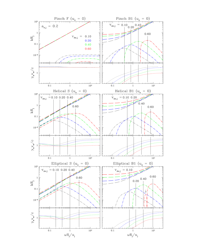
Figure 5: Solutions to the dispersion relation for pinch fundamental, helical surface, elliptical surface (left column) and the first body (right column) modes are shown for equal sound speeds in jet and sheath and no sheath flow. Pinch fundamental mode sound speed is $a_{j,e}=0.2~{}c$. Sound speeds for all other cases are $a_{j,e}\sim 0.01v_{Aj,e}$. Real and imaginary parts of the wavenumber as a function of angular frequency are shown as in Figure 4. Locations of the maximum growth rate are indicated by the vertical solid lines. A vertical arrow (elliptical B1) indicates a narrow damping feature. The underlying panel shows the relativistic wave speed, $\gamma_{w}v_{w}/c$. Line colors indicate the Alfvén speed in units of c: (black) 0.10, (blue) 0.20, (green) 0.40, & (red) 0.60.

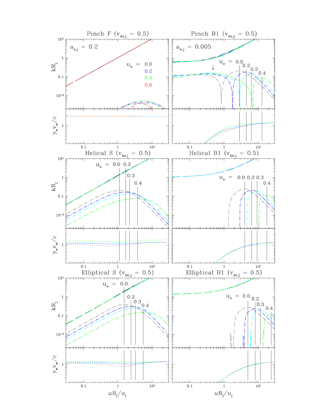
Figure 6: Solutions to the dispersion relation for pinch fundamental, helical surface, elliptical surface (left column) and the first body (right column) modes are shown for equal sound speeds in jet and sheath for different sheath flow speeds. The pinch fundamental mode sound speed is $a_{j,e}=0.2~{}c$. Sound speeds for all other cases are $a_{j,e}\sim 0.01v_{Aj,e}=0.005~{}c$. Real and imaginary parts of the wavenumber as a function of angular frequency are shown as in Figure 4. Locations of the maximum growth rate are indicated by the vertical solid lines. A vertical arrow indicates low frequency damping of the pinch B1 solutions. The underlying panel shows the relativistic wave speed, $\gamma_{w}v_{w}/c$. Line colors indicate the sheath speed in units of c: (black) 0.0, (blue) 0.20, (cyan) 0.30, (green) 0.40, & (red) 0.60.

the pinch fundamental mode panel in order to illustrate the mode behavior with increasing Alfvén speed. Sound speeds for all body modes and for helical and elliptical surface modes are $a_{j,e}\sim 0.01v_{Aj,e}$. Here the transition from super-Alfvénic towards trans-Alfvénic behavior for no flow in the sheath is illustrated. At low frequencies the modes behave as predicted by the analytic solutions given in §3.1. The growth rate of the pinch fundamental mode is reduced as the Alfvén speed increases as predicted by eq. (6). The surface and body mode solutions show the expected shift to a higher resonant frequency that is primarily a function of the increased sheath Alfvén speed and an accompanying increase in the resonant growth rate that is primarily a function of the increased spine Alfvén speed. The resonance moves to higher frequency but the maximum growth rate is reduced for Alfvén speeds $v_{Aj,e}>0.60~{}c$ and all modes become stable at higher Alfvén speeds in accordance with eqs. (8 & 24). At high frequencies wave speeds are given by eq. (26). Provided the jet is sufficiently super-Alfvénic, i.e., $v_{Aj,e}<0.6~{}c$, the maximum growth rate of the first body mode is much greater than that of the pinch fundamental mode, is comparable to that of the helical surface mode, and is less than that of the elliptical surface mode. A narrow damping peak shown for the elliptical body mode (B1) solution when $v_{Aj,e}=0.6~{}c$ indicated by the arrow is indicative of complexities in the body mode solution structure.

Figure 6 illustrates the behavior of fundamental/surface and first body modes as a function of the sheath speed for an equal Alfvén speed in spine and sheath of $v_{Aj,e}=0.5~{}c$. For this value of the Alfvén speeds a sheath speed $u_{e}=0$ provides a super-Alfvénic solution structure baseline. The sound speed is $a_{j,e}=0.2~{}c$ for the pinch fundamental mode panel in order to illustrate the mode behavior with increasing sheath speed. Sound speeds for all other cases are $a_{j,e}\sim 0.01v_{Aj,e}$. Solutions in the first pinch body mode panel show the damping solution as opposed to the purely real solution at the lower frequencies (indicated by the arrow). At higher frequencies the body mode is growing. At low frequencies the surface modes behave as predicted by the analytic solutions given in §3.1 and the growth rate of the surface modes decreases as $u_{e}$ increases. Additionally, the growth rate at resonance decreases as expected for this relatively high Alfvén speed as the sheath speed increases. At the higher frequencies wave speeds are identical, with wave speeds given by eq. (26). Note that the high frequency wave speeds are relatively independent of $u_{e}$. When the velocity shear speed drops to less than the “surface” Alfvén speed, see eq. (11b), the helical and elliptical surface modes and the first body modes are stabilized. This surface and body mode mode stabilization occurs when sheath speeds exceed $u_{e}\sim 0.5~{}c$. However, note that the maximum pinch fundmental mode growth rate is insensitive to the sheath speed and remains unstable at $u_{e}=0.6~{}c$ even when all other modes are stabilized.

4.3 A High Sound and Alfvén Speed Magnetosonic Case

In this subsection the basic behavior of the pinch fundamental, helical surface, elliptical surface and associated first body modes is illustrated for different sheath speeds.

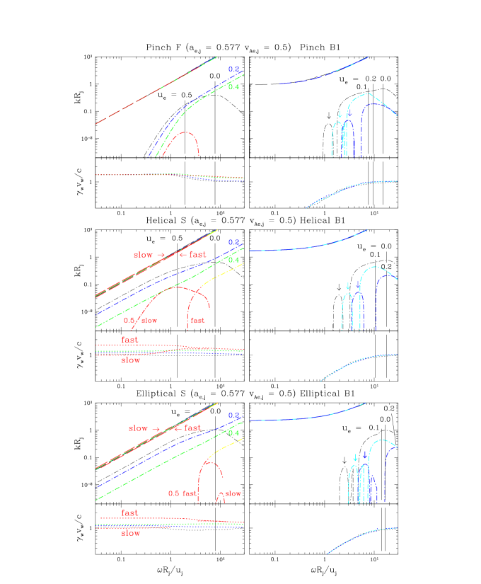
Figure 7: Solutions to the dispersion relation for pinch fundamental, helical surface, elliptical surface (left column), and the associated first body (right column) modes are shown for a maximal spine and sheath sound speed, $a_{j,e}=0.577~{}c$, and a slightly smaller spine and sheath Alfvén speed, $v_{Aj,e}=0.5~{}c$, for different sheath flow speeds. As in previous figures the real part of the wavenumber, $k_{r}R_{j}$, is shown by the dashed lines, the imaginary part , $k_{i}R_{j}$, is shown by the dash-dot lines, and the vertical lines indicate the location of maximum growth. Arrows indicate damping features. The underlying panel shows the relativistic wave speed, $\gamma_{w}v_{w}/c$. Line colors indicate the sheath speed in units of c: (black) 0.0, (blue) 0.20, (green) 0.40, & (red) 0.50. Fast and slow refer to the faster and slower moving solutions and the yellow extension indicates a damped solution.

The sheath speeds span a solution structure from supersonic to transonic but still super-Alfvénic flow. Here the sound speed in jet spine and external sheath are set equal with $a_{j,e}=0.577~{}c$ and Alfvén speeds are set equal with $v_{Aj,e}=0.5~{}c$. The solutions for this case are shown in Figure 7. With no sheath flow the fundamental/surface and first body modes show a typical supersonic and super-Alfvénic structure albeit the pinch fundamental mode now has a maximum growth rate comparable to the helical and elliptical surface modes as a consequence of the high sound speed. The associated first body modes also have maximum growth rates comparable to the fundamental/surface modes. Increase in the sheath speed results in a decrease in the growth rate of the helical and elliptical surface modes at low frequencies as predicted by eq. (8). The low frequency growth rate of the pinch fundamental also declines with increasing sheath speed. The resonant frequency increases with increasing sheath speed as expected from the analytical and numerical studies performed in the fluid and magnetic limits and the fundamental/surface modes take on a transonic structure for sheath speeds $0.4~{}c\leq u_{e}\leq 0.1~{}c$.

At high frequencies the fundamental/surface modes exhibit very high growth rates provided sheath flow remains below the Alfvén speed. On the other hand, the maximum growth rate of the first body modes declines as the sheath speed increases and is reduced severely when $u_{e}>0.1~{}c$. This behavior is similar to what is found for non-relativistic jets as flow enters the transonic and super-Alfvénic regime (Hardee & Rosen 1999). Additional increase in the sheath flow speed to $u_{e}>0.4~{}c$ results in a decrease in the growth rate of the fundamental/surface modes. Solutions for the helical and elliptical surface modes shown in Figure 7 for a sheath speed $u_{e}=0.5~{}c$ equal to the Alfvén speed illustrate some of the complexity associated with barely super-Alfvénic flow. Here limited growth is associated with both the slow and fast helical and elliptical surface solution pair. At slower sheath speeds in the super-Alfvénic regime growth is associated with the slow surface solution, i.e., backwards moving in the jet fluid reference frame. The yellow dash-dot line extension at higher frequencies in the helical and elliptical surface panels indicates a damped solution. Solutions were very difficult to follow in this parameter regime and it is possible that some solutions were not found. When the sheath speed $u_{e}>0.5~{}c$ all modes are stabilized.

A choice of Alfvén speeds greater than sound speeds results in a more magnetic like solution structure like that shown in §4.2. A choice of Alfvén speeds more than a factor of two less than sound speeds produces a more fluid like solution structure like that shown in §4.1. The more complicated solution structure illustrated in Figure 7 only occurs for a relatively narrow range of high sound speeds with similar or slightly lesser Alfvén speeds. In general, the detailed solution structure for situations in which sound and Alfvén speeds are comparable must by examined individually, e.g., Mizuno, Hardee & Nishikawa (2006), and further investigation of these cases is beyond the scope of the present paper.

5 Summary

The analytical and numerical work performed here provides for the first time a detailed analysis of the KH stability properities of a RMHD jet spine-sheath configuration that allows for relativistic motions of the sheath, sound speeds up to $c/\sqrt{3}$, and, by keeping the displacement current in the analysis, Alfvén wave speeds approaching lightspeed and large Alfvén Lorentz factors. In the fluid limit, the present results confirm an earlier more restricted low frequency analytical and numerical simulation study performed by Hardee & Hughes (2003). Provided the jet spine is super-sonic and super-Alfvénic internally and also relative to the sheath, the helical, elliptical and higher order surface modes and the pinch, helical, elliptical and higher order first body modes have a maximum growth rate at a resonant frequency. The pinch fundamental growth rate is significant only when the sound speeds, $a_{j,e}\sim c/\sqrt{3}$. In general, the first body mode maximum growth rate is: greater than the pinch fundamental mode, slightly greater than the helical surface mode, slightly less than the elliptical surface mode, and occurs at a higher frequency than the maximum growth rate for the fundamental/surface mode.

The basic KH stability behavior as a function of spine-sheath parameters is indicated by the analytic low frequency surface mode solution and by the behavior of the resonant frequency. The analytic surface mode solution valid at frequencies below resonance is given by

$$\frac{\omega}{k}=\frac{\omega_{r}}{k}\pm i\frac{\omega_{i}}{k}=\frac{\left[\eta u_{j}+u_{e}\right]\pm i\eta^{1/2}\left[\left(u_{j}-u_{e}\right)^{2}-V_{As}^{2}/\gamma_{j}^{2}\gamma_{e}^{2}\right]^{1/2}}{(1+V_{Ae}^{2}/\gamma_{e}^{2}c^{2})+\eta(1+V_{Aj}^{2}/\gamma_{j}^{2}c^{2})}$$ (27)

where

$$V_{As}^{2}\equiv\left(\gamma_{Aj}^{2}W_{j}+\gamma_{Ae}^{2}W_{e}\right)\frac{B_{j}^{2}+B_{e}^{2}}{4\pi W_{j}W_{e}}~{},$$ (28)

and $\eta\equiv\gamma_{j}^{2}W_{j}\left/\gamma_{e}^{2}W_{e}\right.$, $V_{A}^{2}\equiv B^{2}/4\pi W$, $W\equiv\rho+\left[\Gamma/\left(\Gamma-1\right)\right]P/c^{2}$ and $\gamma_{A}\equiv(1-v_{A}^{2}/c^{2})^{-1/2}$. Equation (27) provides a temporal growth rate, $\omega_{i}(k)$, and a wave speed, $v_{w}=\omega_{r}/k$. The reciprocal provides a spatial growth rate $k_{i}(\omega)$, and growth length $\ell=k_{i}^{-1}$. Increase or decrease of the growth rate, dependence on physical parameters and stabilization at frequencies/wavenumbers below resonance is directly revealed by $\omega_{i}$ in eq. (27). Note that higher jet Lorentz factors reduce $\omega_{i}$ through the dependence on $\eta$.

The resonant frequency is

$$\omega^{\ast}\propto\frac{v_{we}}{\left[\left(1-u_{e}/v^{\ast}_{w}\right)^{2}-\left(v_{we}/v^{\ast}_{w}-u_{e}v_{we}/c^{2}\right)^{2}\right]^{1/2}}~{},$$ (29)

where $v_{w}^{\ast}$ is the wave speed at resonance, eq. (15). The resonant frequency increases as the sheath sound or Alfvén wave speed, $v_{we}\equiv(a_{e},v_{Ae})$ increases and $\omega^{\ast}\longrightarrow\infty$ when the denominator decreases to zero as

$$\frac{u_{j}-u_{e}}{1-u_{j}u_{e}/c^{2}}\longrightarrow\frac{v_{wj}+v_{we}}{1+v_{wj}v_{we}/c^{2}}~{},$$

where $v_{wj,e}\equiv(a_{j,e},v_{Aj,e})$ in the fluid and magnetic limits, respectively. Since eq. (27) applies below resonance the overall behavior of the growth rate is indicated by $\omega_{i}$. Thus, growth rates decline to zero as $(u_{j}-u_{e})^{2}-V_{As}^{2}/\gamma_{j}^{2}\gamma_{e}^{2}\longrightarrow 0$. The numerical analysis of the dispersion relation shows that the pinch fundamental and all first body modes are comparably or more readily stabilized and thus the jet is KH stable when

$$\left(u_{j}-u_{e}\right)^{2}-V_{As}^{2}/\gamma_{j}^{2}\gamma_{e}^{2}<0~{}.$$ (30)

This stability condition takes on a particularly simple form when conditions in spine and sheath are equal, i.e., $B_{e}=B_{j}$, $W_{e}=W_{j}$, so that $v_{A,j}=v_{A,e}$, and with $\gamma_{A}\equiv\gamma_{A,e}=\gamma_{A,j}$

$$\gamma_{j}^{2}\gamma_{e}^{2}\left(u_{j}-u_{e}\right)^{2}<4\gamma_{A}^{2}\left(\gamma_{A}^{2}-1\right)c^{2}$$ (31)

indicates stability. This result implies that a trans-Alfvénic relativistic jet with $\gamma_{j}u_{j}\gtrsim\gamma_{A}v_{A}$ will be KH stable, and that even a super-Alfvénic jet with $\gamma_{j}>>\gamma_{A}$ can be KH stable.

6 Discussion

Formally, the present results and expressions apply only to magnetic fields parallel to an axial spine-sheath flow in which conditions within the spine and within the sheath are independent of radius and the sheath extends to infinity. A rapid decline in perturbation amplitudes in the sheath as a function of radius, governed by the Hankel function in the dispersion relation, suggests that the present results will apply to sheaths more than about three times the spine radius in thickness.

The relativistic jet is transonic in the absence of sheath flow only for spine and sheath sound speeds $\sim c/\sqrt{3}$. Only in this regime does the pinch fundamental have a significant growth rate and, in general, we do not expect the pinch fundamental to grow significantly on relativistic jets. On the other hand, the pinch first body mode can have a significant maximum growth rate and would dominate any axisymmetric structure. The elliptical and higher order surface modes have increasingly larger maximum growth rates at resonant frequencies higher than the helical surface mode, and the maximum first body mode growth rates for helical and elliptical modes are comparable to that of the surface modes. Nevertheless, we expect the helical surface mode to achieve the largest amplitudes in the non-linear limit as a result of the reduced saturation amplitudes that accompany the higher resonant frequency and shorter resonant wavelengths associated with the higher order surface modes and all body modes.

In astrophysical jets we expect a toroidal magnetic field component, and possibly an ordered helical structure and accompanying flow helicity. Jet rotation (e.g., Bodo et al. 1996), or a radial velocity profile (e.g., Birkinshaw 1991) will modify the present results but will not stabilize the helical mode. Two dimensional non-relativistic slab jet theoretical results, indicate that KH stabilization occurs when the velocity shear projected on the wavevector is less than the projected Alfvén speed (Hardee et al. 1992). In the work presented here magnetic and flow field are parallel and project equally on the wavevector which for the helical (n = 1) and elliptical (n = 2) mode lies at an angle $\theta=tan^{-1}(n/kR)$ relative to the jet axis. Provided magnetic and flow helicity and radial gradients in jet spine/sheath properties are not too large we expect the present results to remain valid where $u_{j,e}$ and $B_{j,e}$ refer to the poloidal velocity and field components.

KH driven normal mode structures move at less than the jet speed. The fundamental pinch mode moves backwards in the jet frame at about the sound speed nearly independent of the sheath properites and thus moves at nearly the jet speed in the source/observer frame. Low frequency and long wavelength helical and higer order surface modes are advected with wave speed indicated by eq. (27) and move slowly in the source/observer frame for light, i.e. $\eta\equiv\gamma_{j}^{2}W_{j}\left/\gamma_{e}^{2}W_{e}\right.<1$, and/or for magnetically dominated flows. Higher frequency (above resonance) and shorter wavelength normal mode structures move backwards in the jet frame at the sound/Alfvén wave speed, have a wave speed nearly independent of the sheath properties, and can move slowly in the source/observer frame only for magnetically dominated flows.

Where flow and magentic fields are parallel, current driven (CD) modes are stable (Isotomin & Pariev 1994, 1996). Where magnetic and flow fields are helical CD modes can be unstable (Lyubarskii 1999) in addition to the KH modes. CD and KH instability are expected to produce helically twisted structure. However, the conditions for instability, the radial structure, the growth rate and the pattern motions are different. For example, KH modes grow more rapidly when the magnetic field is force-free (e.g., Appl 1996), and non-relativistic simulation work (e.g., Lery et al. 2000; Baty & Keppens 2003; Nakamura & Meier 2004) indicates that CD driven structure is internal to any spine-sheath interface and moves at the jet speed.

The differences between KH and CD instability can serve to identify the source of helical structure on relativistic jets and allow determination of jet properties near to the central engine. Perhaps the observation of relatively low proper motions in the TeV BL Lacs when intensity modeling requires high flow Lorentz factors (Ghisellini et al. 2005) is an indication of a magnetically dominated KH unstable spine-sheath configuration.

Appendix A Linearization of the RMHD Equations

In vector notation the relativistic MHD continuity equation, energy equation, and momentum equation can be written as:

$$\frac{\partial}{\partial t}\left[\gamma\rho\right]+\mathbf{\nabla}\cdot\left[\gamma\rho\mathbf{v}\right]=0~{},$$ (A1)

$$\frac{\partial}{\partial t}\left[\gamma^{2}W-\frac{P}{c^{2}}+\frac{B^{2}}{8\pi c^{2}}(1+\frac{v^{2}}{c^{2}})-\frac{(\mathbf{v}/c\cdot\mathbf{B})^{2}}{8\pi c^{2}}\right]+\mathbf{\nabla}\cdot\left[\gamma^{2}W\mathbf{v}+\frac{B^{2}}{4\pi c^{2}}\mathbf{v-}(\mathbf{v}\cdot\mathbf{B})\frac{\mathbf{B}}{4\pi c^{2}}\right]=0~{},$$ (A2)

and

$$\gamma^{2}W\left(\frac{\partial}{\partial t}\mathbf{v}+\mathbf{v}\cdot\nabla\mathbf{v}\right)=-\mathbf{\nabla}P-\frac{\mathbf{v}}{c^{2}}\frac{\partial}{\partial t}P+\rho_{q}\mathbf{E}+\frac{\left[\mathbf{j}\times\mathbf{B}\right]}{4\pi}~{}.$$ (A3)

These equations along with Maxwell’s equations

$$\begin{array}[]{cc}\mathbf{\nabla}\cdot\mathbf{B}=0&\mathbf{\nabla}\cdot\mathbf{E}=4\pi\rho_{q}\\ \mathbf{\nabla}\times\mathbf{B}=\frac{1}{c}\frac{\partial}{\partial t}\mathbf{E}+\frac{4\pi}{c}\mathbf{j}&\mathbf{\nabla}\times\mathbf{E}=-\frac{1}{c}\frac{\partial}{\partial t}\mathbf{B}\end{array}$$

and assuming ideal MHD with comoving electric field equal to zero

$$\mathbf{E=-}\frac{\mathbf{v}\times\mathbf{B}}{c}~{},$$

provide the complete set of ideal RMHD equations. In the above $W$ is the enthalpy, the Lorentz factor $\gamma=(1-\mathbf{v\cdot v}/c^{2})^{-1/2}$, and $\rho$ is the proper density. In what follows I will assume that the effects of radiation can be ignored, the enthalpy is given by

$$W=\rho+\frac{\Gamma}{\Gamma-1}\frac{P}{c^{2}}~{},$$

and the condition for isentropic flow is given by

$$\left(\frac{\partial}{\partial t}+\mathbf{v\cdot\nabla}\right)\left(\frac{P}{\rho^{\Gamma}}\right)=0~{}.$$

The general approach to analyzing the time dependent properties of this system is to linearize the ideal RMHD equations, where the density, velocity, pressure and magnetic field are written as $\rho=\rho_{0}+\rho_{1}$, $\mathbf{v}=\mathbf{u}+\mathbf{v}_{1}$ (we use $\mathbf{v}_{0}\equiv\mathbf{u}$ for notational reasons), $P=P_{0}+P_{1}$ $\mathbf{E}=\mathbf{E}_{0}+\mathbf{E}_{1}$, and $\mathbf{B}=\mathbf{B}_{0}+\mathbf{B}_{1}$, where subscript 1 refers to a perturbation to the equilibrium quantity with subscript 0. Additionally, $W=W_{0}+W_{1}$, $\gamma^{2}=(\gamma_{0}+\gamma_{1})^{2}\simeq\gamma_{0}^{2}+2\gamma_{0}^{4}\mathbf{u\cdot v}_{1}/c^{2}$ and $\gamma_{1}\simeq\gamma_{0}^{3}\mathbf{u\cdot v}_{1}/c^{2}$.  It is assumed that the initial equilibrium system satisfies the zero order equations. The linearized continuity, energy and momentum equation become

$$\frac{\partial}{\partial t}\left[\gamma_{0}\rho_{1}+\gamma_{1}\rho_{0}\right]+\mathbf{\nabla}\cdot\left[\gamma_{0}\rho_{1}\mathbf{u}+\gamma_{0}\rho_{0}\mathbf{v}_{1}+\gamma_{1}\rho_{0}\mathbf{u}\right]=0~{},$$ (A4)

$$\begin{array}[]{c}\frac{\partial}{\partial t}\left[\gamma_{0}^{2}W_{1}-P_{1}/c^{2}+2\gamma_{0}^{4}\left(\mathbf{u}\cdot\mathbf{v}_{1}/c^{2}\right)W_{0}\right]+\mathbf{\nabla}\cdot\left[\gamma_{0}^{2}W_{1}\mathbf{u}+2\gamma_{0}^{4}\left(\mathbf{u}\cdot\mathbf{v}_{1}/c^{2}\right)W_{0}\mathbf{u}+\gamma_{0}^{2}W_{0}\mathbf{v}_{1}\right]\\ +\frac{1}{4\pi c^{2}}\frac{\partial}{\partial t}\left[B_{0}^{2}\left(\mathbf{u}\cdot\mathbf{v}_{1}/c^{2}\right)+(1+u^{2}/c^{2})\mathbf{B}_{0}\mathbf{\cdot B}_{1}-(\mathbf{u\cdot B}_{1}/c+\mathbf{v}_{1}\mathbf{\cdot B}_{0}/c)\mathbf{u\cdot B}_{0}/c\right]\\ +\frac{1}{4\pi c^{2}}\mathbf{\bigtriangledown}\cdot\left[2(\mathbf{B}_{0}\mathbf{\cdot B}_{1})\mathbf{u+}B_{0}^{2}\mathbf{v}_{1}-(\mathbf{u\cdot B}_{0})\mathbf{B}_{1}-(\mathbf{u\cdot B}_{1})\mathbf{B}_{0}-(\mathbf{v}_{1}\mathbf{\cdot B}_{0})\mathbf{B}_{0}\right]=0~{},\end{array}$$

and

$$\gamma_{0}^{2}W_{0}\left(\frac{\partial\mathbf{v}_{1}}{\partial t}+\mathbf{u}\cdot\nabla\mathbf{v}_{1}\right)=-\mathbf{\nabla}P_{1}-\frac{\mathbf{u}}{c^{2}}\frac{\partial P_{1}}{\partial t}+\frac{(\mathbf{j}_{0}\mathbf{\times B}_{1})+(\mathbf{j}_{1}\mathbf{\times B}_{0})}{c}~{}.$$ (A5)

The linearized Maxwell equations become:

$$\begin{array}[]{cc}\mathbf{\nabla}\cdot\mathbf{B}_{1}=0&\mathbf{\nabla}\cdot\mathbf{E}_{1}=4\pi\rho_{q1}\\ \mathbf{\nabla}\times\mathbf{B}_{1}=\frac{1}{c}\frac{\partial}{\partial t}\mathbf{E}_{1}+\frac{4\pi}{c}\mathbf{j}_{1}&\mathbf{\nabla}\times\mathbf{E}_{1}=-\frac{1}{c}\frac{\partial}{\partial t}\mathbf{B}_{1}\end{array}$$

where I keep the displacement current in order to allow for strong magnetic fields and Alfvén wave speeds comparable to lightspeed. Under the assumption of ideal MHD, the comoving electric field is zero, the equilibrium charge density $\rho_{q,0}=0$, and the electric field

$$\mathbf{E}_{1}\mathbf{=-}\frac{\mathbf{u}\times\mathbf{B}_{1}+\mathbf{v}_{1}\mathbf{\times B}_{0}}{c}~{},$$

is first order, the charge density $\rho_{q1}=\left(\mathbf{\bigtriangledown}\cdot\mathbf{E}_{1}\right)\mathbf{/}4\pi$ is also first order, and the electrostatic force term, $\rho_{q1}\mathbf{E}_{1}$, is second order and dropped from the linearized momentum equation. The condition for isentropic perturbations becomes

$$P_{1}=\tilde{a}^{2}\rho_{1}=\left(\Gamma\frac{P_{0}}{\rho_{0}}\right)\rho_{1}~{}.$$

This basic set of linearized RMHD equations is similar to those found in Begelman (1998) but allows a relativistic zeroth order velocity, i.e., $\mathbf{v}=\mathbf{u}+\mathbf{v_{1}}$ and $\mathbf{u}\lesssim c$ whereas Begelman allowed only for relativistic first order motions, $\mathbf{v_{1}}$.

In what follows let us model a jet as a cylinder of radius R, having a uniform proper density, $\rho_{j}$, a uniform axial magnetic field, $B_{j}=B_{z,j}$, and a uniform velocity, $u_{j}=u_{z,j}$. The external medium is assumed to have a uniform proper density, $\rho_{e}$, a uniform axial magnetic field, $B_{e}=B_{z,e}$, and a uniform velocity, $u_{e}=u_{z,e}$. An external velocity could be the result of a wind or sheath outflow around a central jet, $u_{e}>0$, or could represent backflow, $u_{e}<0$, in a cocoon surrounding the jet. The jet is established in static total pressure balance with the external medium where the total static uniform pressure is $P_{e}^{\ast}\equiv P_{e}+B_{e}^{2}/8\pi=P_{j}^{\ast}\equiv P_{j}+B_{j}^{2}/8\pi$.  Under these assumptions the linearized continuity equation becomes

$$\frac{\partial}{\partial t}\left[\gamma_{0}\rho_{1}+\gamma_{1}\rho_{0}\right]+u\frac{\partial}{\partial z}\left[\gamma_{0}\rho_{1}+\gamma_{1}\rho_{0}\right]+\gamma_{0}\rho_{0}\mathbf{\nabla}\cdot\mathbf{v}_{1}=0~{}.$$ (A6)

The linearized energy equation becomes

$$\frac{\partial}{\partial t}\left[\gamma_{0}^{2}W_{1}-\frac{P_{1}}{c^{2}}+2\gamma_{0}^{4}\frac{uv_{z1}}{c^{2}}W_{0}\right]+u\frac{\partial}{\partial z}\left[\gamma_{0}^{2}W_{1}+2\gamma_{0}^{4}\frac{uv_{z1}}{c^{2}}W_{0}\right]+\gamma_{0}^{2}W_{0}\mathbf{\nabla}\cdot\mathbf{v}_{1}=0~{}.$$ (A7)

This result for the linearized energy equation is found by noting that the magnetic terms in the energy equation linearize to

$$\begin{array}[]{c}B_{0}\left[\frac{\partial}{\partial t}B_{z1}+u\frac{\partial}{\partial z}B_{z1}\right]-(uB_{0})\mathbf{\nabla}\cdot\mathbf{B}_{1}+B_{0}^{2}\mathbf{\nabla}\cdot\mathbf{v}_{1}-B_{0}^{2}\frac{\partial}{\partial z}v_{z1}=\\ -B_{0}^{2}\left[\mathbf{\nabla}\cdot\mathbf{v}_{1}-\frac{\partial}{\partial z}v_{z1}\right]+B_{0}^{2}\left[\mathbf{\nabla}\cdot\mathbf{v}_{1}-\frac{\partial}{\partial z}v_{z1}\right]=0\end{array}$$

where I have used

$$\frac{\partial}{\partial t}B_{z1}+u\frac{\partial}{\partial z}B_{z1}=-\frac{B_{0}}{r}\left[\frac{\partial}{\partial r}(rv_{r1})+\frac{\partial}{\partial\phi}v_{\phi 1}\right]=-B_{0}\left[\mathbf{\nabla}\cdot\mathbf{v}_{1}-\frac{\partial}{\partial z}v_{z1}\right]$$

from $\partial\mathbf{B}_{1}/\partial t=\mathbf{\nabla\times}\left(\mathbf{u\times B}_{1}\right)+\mathbf{\nabla\times}\left(\mathbf{v}_{1}\mathbf{\times B}_{0}\right)$. The linearized momentum equation becomes

$$\begin{array}[]{c}\gamma_{0}^{2}W_{0}\left[\frac{\partial}{\partial t}\mathbf{v}_{1}+\mathbf{u}\cdot\nabla\mathbf{v}_{1}-\frac{1}{4\pi c^{2}\gamma_{0}^{2}W_{0}}\left(\frac{\partial}{\partial t}\mathbf{v}_{1}\mathbf{\times B}_{0}\right)\mathbf{\times B}_{0}\right]=\\ -\mathbf{\bigtriangledown}P_{1}-\frac{\mathbf{u}}{c^{2}}\frac{\partial}{\partial t}P_{1}+\frac{1}{4\pi}\left[(\bigtriangledown\times\mathbf{B}_{0})\times\mathbf{B}_{1}+(\bigtriangledown\times\mathbf{B}_{1})\times\mathbf{B}_{0}\right]+\frac{1}{4\pi c^{2}}\left(\mathbf{u\times}\frac{\partial}{\partial t}\mathbf{B}_{1}\right)\mathbf{\times B}_{0}\end{array}$$ (A8)

where I have used

$$\frac{\mathbf{j}_{0}\mathbf{\times B}_{1}}{c}=\frac{(\mathbf{\nabla\times B}_{0})\mathbf{\times B}_{1}}{4\pi}~{},$$

and

$$\frac{\mathbf{j}_{1}\mathbf{\times B}_{0}}{c}=\frac{(\mathbf{\nabla\times B}_{1})\mathbf{\times B}_{0}}{4\pi}-\frac{1}{4\pi c}\frac{\partial}{\partial t}\mathbf{E}_{1}\mathbf{\times B}_{0}=\frac{(\mathbf{\nabla\times B}_{1})\mathbf{\times B}_{0}}{4\pi}+\frac{1}{4\pi c^{2}}\left(\mathbf{u}\times\frac{\partial}{\partial t}\mathbf{B}_{1}+\frac{\partial}{\partial t}\mathbf{v}_{1}\mathbf{\times B}_{0}\right)\mathbf{\times B}_{0}~{},$$

which includes the displacement current. The components of the linearized momentum equation can be written as

$$\gamma_{0}^{2}W_{0}\left[\left(1+\frac{V_{A}^{2}}{\gamma_{0}^{2}c^{2}}\right)\frac{\partial}{\partial t}v_{r1}+u\frac{\partial}{\partial z}v_{r1}\right]=-\frac{\partial}{\partial r}P_{1}+\frac{B_{0}}{4\pi}\left(\frac{\partial}{\partial z}B_{r1}+\frac{u}{c^{2}}\frac{\partial}{\partial t}B_{r1}-\frac{\partial}{\partial r}B_{z1}\right)~{},$$ ()

$$\gamma_{0}^{2}W_{0}\left[\left(1+\frac{V_{A}^{2}}{\gamma_{0}^{2}c^{2}}\right)\frac{\partial}{\partial t}v_{\phi 1}+u\frac{\partial}{\partial z}v_{\phi 1}\right]=-\frac{1}{r}\frac{\partial}{\partial\phi}P_{1}+\frac{B_{0}}{4\pi}\left(\frac{\partial}{\partial z}B_{\phi 1}+\frac{u}{c^{2}}\frac{\partial}{\partial t}B_{\phi 1}-\frac{1}{r}\frac{\partial}{\partial\phi}B_{z1}\right)~{},$$ ()

and

$$\gamma_{0}^{2}W_{0}\left[\frac{\partial}{\partial t}v_{z1}+u\frac{\partial}{\partial z}v_{z1}\right]=-\frac{\partial}{\partial z}P_{1}-\frac{u}{c^{2}}\frac{\partial}{\partial t}P_{1}$$ ()

where $V_{A}^{2}\equiv B_{0}^{2}/(4\pi W_{0})$.

Appendix B Normal Mode Dispersion Relation

In cylindrical geometry perturbations $\rho_{1}$, $\bf{v}_{1}$, $P_{1}$, and $\bf{B}_{1}$ can be considered to consist of Fourier components of the form

$$f_{1}(r,\phi,z,t)=f_{1}(r)e^{i(kz\pm n\phi-\omega t)}$$

where the flow is in the $z$ direction, and $r$ is in the radial direction with the jet bounded by $r=R$. In cylindrical geometry $n$, an integer, is the azimuthal wavenumber, for $n>0$ waves propagate at an angle to the flow direction, where $+n$ and $-n$ refer to wave propagation in the clockwise and counterclockwise sense, respectively, when viewed outwards along the flow direction. In general the goal is to write a differential equation for the radial dependence of the total pressure perturbation $P_{1}^{\ast}\equiv P_{1}+(\mathbf{B}_{1}\cdot\mathbf{B}_{0})/4\pi=P_{1}^{\ast}(r)\exp[i(kz\pm n\phi-\omega t)]$. The differential equation can be obtained from the energy equation by using the momentum equation and writing the velocity components $v_{r1},v_{\phi 1},v_{z1}$ in terms of $P_{1}^{\ast},u,B_{0}$. The components of the linearized momentum equation (eqs. A10a, b, & c) written in the form

$$\gamma_{0}^{2}W_{0}\left[\left(1+\frac{V_{A}^{2}}{\gamma_{0}^{2}c^{2}}\right)\frac{\partial}{\partial t}v_{r1}+u\frac{\partial}{\partial z}v_{r1}\right]=-\frac{\partial}{\partial r}P_{1}^{\ast}+\frac{B_{0}}{4\pi}\left(\frac{\partial}{\partial z}B_{r1}+\frac{u}{c^{2}}\frac{\partial}{\partial t}B_{r1}\right)~{},$$ ()

$$\gamma_{0}^{2}W_{0}\left[\left(1+\frac{V_{A}^{2}}{\gamma_{0}^{2}c^{2}}\right)\frac{\partial}{\partial t}v_{\phi 1}+u\frac{\partial}{\partial z}v_{\phi 1}\right]=-\frac{1}{r}\frac{\partial}{\partial\phi}P_{1}^{\ast}+\frac{B_{0}}{4\pi}\left(\frac{\partial}{\partial z}B_{\phi 1}+\frac{u}{c^{2}}\frac{\partial}{\partial t}B_{\phi 1}\right)~{},$$ ()

and

$$\gamma_{0}^{2}W_{0}\left[\frac{\partial}{\partial t}v_{z1}+u\frac{\partial}{\partial z}v_{z1}\right]=-\left(\frac{\partial}{\partial z}P_{1}^{\ast}+\frac{u}{c^{2}}\frac{\partial}{\partial t}P_{1}^{\ast}\right)+\frac{B_{0}}{4\pi}\left(\frac{\partial}{\partial z}B_{z1}+\frac{u}{c^{2}}\frac{\partial}{\partial t}B_{z1}\right)$$ ()

along with

$$\frac{\partial}{\partial t}\mathbf{B}_{1}=-c(\mathbf{\nabla}\times\mathbf{E}_{1})=\mathbf{\nabla\times}(\mathbf{u\times B}_{1})+\mathbf{\nabla\times}(\mathbf{v}_{1}\mathbf{\times B}_{0})$$

are used to provide relations between $B_{r1}$ and $v_{r1}$, and $B_{\phi 1}$ and $v_{\phi 1}$

$$\frac{\partial}{\partial t}B_{r1}+u\frac{\partial}{\partial z}B_{r1}=B_{0}\frac{\partial}{\partial z}v_{r1}~{},$$ ()

$$\frac{\partial}{\partial t}B_{\phi 1}+u\frac{\partial}{\partial z}B_{\phi 1}=B_{0}\frac{\partial}{\partial z}v_{\phi 1}~{},$$ ()

and to provide a relation between $B_{z1}$, $v_{z1}$, and $P_{1}^{\ast}$

$$\begin{array}[]{c}\left[1+\frac{V_{A}^{2}}{c^{2}}\left(\frac{1}{\tilde{a}^{2}}+\frac{\Gamma}{\Gamma-1}\frac{1}{c^{2}}\right)\right]\left[\frac{\partial}{\partial t}B_{z1}+u\frac{\partial}{\partial z}B_{z1}\right]-\frac{V_{A}^{2}}{\gamma_{0}^{2}c^{2}}\frac{\partial}{\partial t}B_{z1}=\\ B_{0}\frac{\partial}{\partial z}v_{z1}+2B_{0}\gamma_{0}^{2}\frac{u}{c^{2}}\left[\frac{\partial}{\partial t}v_{z1}+u\frac{\partial}{\partial z}v_{z1}\right]\\ +\frac{B_{0}}{W_{0}}\left(\frac{1}{\tilde{a}^{2}}+\frac{\Gamma}{\Gamma-1}\frac{1}{c^{2}}\right)\left[\frac{\partial}{\partial t}P_{1}^{\ast}+u\frac{\partial}{\partial z}P_{1}^{\ast}\right]-\frac{B_{0}}{c^{2}\gamma_{0}^{2}W_{0}}\frac{\partial}{\partial t}P_{1}^{\ast}~{}.\end{array}$$ ()

To obtain equation (B2c) I have used

$$\frac{\partial}{\partial t}B_{z1}+u\frac{\partial}{\partial z}B_{z1}=-\frac{B_{0}}{r}\left[\frac{\partial}{\partial r}(rv_{r1})+\frac{\partial}{\partial\phi}v_{\phi 1}\right]=-B_{0}\left[\mathbf{\bigtriangledown}\cdot\mathbf{v}_{1}-\frac{\partial}{\partial z}v_{z1}\right]$$

where

$$-\gamma_{0}^{2}W_{0}\mathbf{\bigtriangledown}\cdot\mathbf{v}_{1}=\gamma_{0}^{2}\left(\frac{1}{\tilde{a}^{2}}+\frac{\Gamma}{\Gamma-1}\frac{1}{c^{2}}\right)\left[\frac{\partial}{\partial t}P_{1}+u\frac{\partial}{\partial z}P_{1}\right]-\frac{1}{c^{2}}\frac{\partial}{\partial t}P_{1}+2\gamma_{0}^{4}\frac{u}{c^{2}}W_{0}\left[\frac{\partial}{\partial t}v_{z1}+u\frac{\partial}{\partial z}v_{z1}\right]$$

from the energy equation (eq. A8), and

$$W_{1}=\rho_{1}+\frac{\Gamma}{\Gamma-1}\frac{P_{1}}{c^{2}}=\left(\frac{1}{\tilde{a}^{2}}+\frac{\Gamma}{\Gamma-1}\frac{1}{c^{2}}\right)P_{1}~{}.$$

Using equations (B1a, b, & c) combined with

$$\begin{array}[]{c}\frac{\partial}{\partial t}f_{1}(r,\phi,z,t)=-i\omega f_{1}(r)e^{i\left(kz\pm n\phi-\omega t\right)}\\ \frac{\partial}{\partial r}f_{1}(r,\phi,z,t)=\frac{\partial}{\partial r}f_{1}(r)e^{i\left(kz\pm n\phi-\omega t\right)}\\ \frac{\partial}{\partial\phi}f_{1}(r,\phi,z,t)=\pm inf_{1}(r)e^{i\left(kz\pm n\phi-\omega t\right)}\\ \frac{\partial}{\partial z}f_{1}(r,\phi,z,t)=+ikf_{1}(r)e^{i\left(kz\pm n\phi-\omega t\right)}\end{array}$$

allows the velocity components to be written as

$$i\gamma_{0}^{2}W_{0}\left[ku-\omega\left(1+\frac{V_{A}^{2}}{\gamma_{0}^{2}c^{2}}\right)\right]v_{r1}=-\frac{\partial}{\partial r}P_{1}^{\ast}+i\frac{B_{0}}{4\pi}\left(k-\omega\frac{u}{c^{2}}\right)B_{r1}~{},$$ ()

$$i\gamma_{0}^{2}W_{0}\left[ku-\omega\left(1+\frac{V_{A}^{2}}{\gamma_{0}^{2}c^{2}}\right)\right]v_{\phi 1}=-\frac{1}{r}\frac{\partial}{\partial\phi}P_{1}^{\ast}+i\frac{B_{0}}{4\pi}\left(k-\omega\frac{u}{c^{2}}\right)B_{\phi 1}~{},$$ ()

and

$$\gamma_{0}^{2}W_{0}\left[ku-\omega\right]v_{z1}=-\left(k-\omega\frac{u}{c^{2}}\right)P_{1}^{\ast}+\frac{B_{0}}{4\pi}\left(k-\omega\frac{u}{c^{2}}\right)B_{z1}~{}.$$ ()

The perturbed magnetic field components from equations (B2a, b,& c) become

$$B_{r1}=\frac{kv_{r1}}{ku-\omega}B_{0}~{},$$ ()

$$B_{\phi 1}=\frac{kv_{\phi 1}}{ku-\omega}B_{0}~{},$$ ()

and

$$B_{z1}=\frac{\frac{1}{W_{0}}\left[\frac{\left(ku-\omega\right)}{a^{2}}-\left(k-\omega u/c^{2}\right)\frac{u}{c^{2}}\right]P_{1}^{\ast}+\gamma_{0}^{2}\left[\left(k-\omega u/c^{2}\right)+\left(ku-\omega\right)\frac{u}{c^{2}}\right]v_{z1}}{\left(ku-\omega\right)+V_{A}^{2}\left[\frac{\left(ku-\omega\right)}{a^{2}}-\left(k-\omega u/c^{2}\right)\frac{u}{c^{2}}\right]}B_{0}$$ ()

where I have used

$$\begin{array}[]{c}k+2\gamma_{0}^{2}\left(ku-\omega\right)u/c^{2}=\gamma_{0}^{2}\left[\left(k-\omega u/c^{2}\right)+\left(ku-\omega\right)u/c^{2}\right]~{},\\ \gamma_{0}^{2}\left(ku-\omega\right)\left[\tilde{a}^{-2}+\Gamma\left(\Gamma-1\right)^{-1}c^{-2}\right]+\omega/c^{2}=\gamma_{0}^{2}\left[\left(ku-\omega\right)/a^{2}-\left(k-\omega u/c^{2}\right)u/c^{2}\right]~{},\end{array}$$

and

$$a^{2}\equiv\left(\frac{1}{\tilde{a}^{2}}+\frac{\Gamma}{\Gamma-1}\frac{1}{c^{2}}-\frac{1}{c^{2}}\right)^{-1}=\frac{\Gamma P}{\rho+\frac{\Gamma}{\Gamma-1}\frac{P}{c^{2}}}$$

to obtain the expression for $B_{z1}$. Using equations (B4a, b, & c) for the perturbed magnetic field components, I obtain the following relations between the perturbed velocity components $\mathbf{v}_{1}$ and the total pressure perturbation $P_{1}^{\ast}$:

$$v_{r1}\equiv C_{r}\frac{\partial}{\partial r}P_{1}^{\ast}=i\frac{1}{X}\frac{\partial}{\partial r}P_{1}^{\ast}=i\frac{\left(ku-\omega\right)}{\gamma_{0}^{2}W_{0}\gamma_{A}^{2}\left[\left(ku-\omega\right)^{2}-\left(k-\omega u/c^{2}\right)^{2}v_{A}^{2}\right]}\frac{\partial}{\partial r}P_{1}^{\ast}~{},$$ ()

$$v_{\phi 1}\equiv C_{\phi}P_{1}^{\ast}=\mp\frac{n}{r}\frac{1}{X}P_{1}^{\ast}=\mp\frac{n}{r}\frac{\left(ku-\omega\right)}{\gamma_{0}^{2}W_{0}\gamma_{A}^{2}\left[\left(ku-\omega\right)^{2}-\left(k-\omega u/c^{2}\right)^{2}v_{A}^{2}\right]}P_{1}^{\ast}~{},$$ ()

and

$$v_{z1}\equiv C_{z}P_{1}^{\ast}=-\frac{\left(ku-\omega\right)\left(k-\omega u/c^{2}\right)}{\gamma_{0}^{2}W_{0}\left\{\left(ku-\omega\right)^{2}+\gamma_{A}^{2}v_{A}^{2}\left[\frac{\left(ku-\omega\right)^{2}}{a^{2}}-\left(k-\omega u/c^{2}\right)^{2}\right]\right\}}P_{1}^{\ast}~{}.$$ ()

To obtain the above relationships I have used

$$\left(ku-\omega\right)-\frac{V_{A}^{2}}{\gamma_{0}^{2}}\left(\frac{k-\omega u/c^{2}}{ku-\omega}k+\frac{\omega}{c^{2}}\right)=\gamma_{A}^{2}\left[\left(ku-\omega\right)-\frac{\left(k-\omega u/c^{2}\right)^{2}}{\left(ku-\omega\right)}v_{A}^{2}\right]$$

in addition to

$$\gamma_{0}^{2}\left(ku-\omega\right)\left[\tilde{a}^{-2}+\Gamma\left(\Gamma-1\right)^{-1}c^{-2}\right]+\omega/c^{2}=\gamma_{0}^{2}\left[\left(ku-\omega\right)/a^{2}-\left(k-\omega u/c^{2}\right)u/c^{2}\right]$$

where

$$v_{A}^{2}\equiv\frac{V_{A}^{2}}{1+V_{A}^{2}/c^{2}}$$

is the Alfvén wave speed and $\gamma_{A}^{2}=\left(1-v_{A}^{2}/c^{2}\right)^{-1}$ is an Alfvénic Lorentz factor. Note that $V_{A}^{2}=\gamma_{A}^{2}v_{A}^{2}$ and $\gamma_{A}^{2}=1+V_{A}^{2}/c^{2}$. Thus we have that

$$\begin{array}[]{c}\mathbf{\nabla}\cdot\mathbf{v}_{1}=C_{r}\frac{\partial^{2}}{\partial r^{2}}P_{1}^{\ast}+\frac{C_{r}}{r}\frac{\partial}{\partial r}P_{1}^{\ast}+\frac{C_{\phi}}{r}\frac{\partial}{\partial\phi}P_{1}^{\ast}+C_{z}\frac{\partial}{\partial z}P_{1}^{\ast}\\ =\frac{i}{X}\frac{\partial^{2}}{\partial r^{2}}P_{1}^{\ast}+\frac{1}{r}\frac{i}{X}\frac{\partial}{\partial r}P_{1}^{\ast}-\frac{n^{2}}{r}\frac{i}{X}P_{1}^{\ast}+ikC_{z}P_{1}^{\ast}~{}.\end{array}$$ (B6)

Using the energy equation (eq. A8) written in the form

$$\begin{array}[]{c}-\gamma_{0}^{2}W_{0}\mathbf{\bigtriangledown}\cdot\mathbf{v}_{1}=\gamma_{0}^{2}\left(\frac{1}{\tilde{a}^{2}}+\frac{\Gamma}{\Gamma-1}\frac{1}{c^{2}}\right)\left[\frac{\partial}{\partial t}P_{1}^{\ast}+u\frac{\partial}{\partial z}P_{1}^{\ast}\right]-\frac{1}{c^{2}}\frac{\partial}{\partial t}P_{1}^{\ast}\\ -\gamma_{0}^{2}\left(\frac{1}{\tilde{a}^{2}}+\frac{\Gamma}{\Gamma-1}\frac{1}{c^{2}}\right)\left[\frac{\partial}{\partial t}B_{z1}+u\frac{\partial}{\partial z}B_{z1}\right]+\frac{1}{c^{2}}\frac{\partial}{\partial t}B_{z1}+2\gamma_{0}^{4}\frac{u}{c^{2}}W_{0}\left[\frac{\partial}{\partial t}v_{z1}+u\frac{\partial}{\partial z}v_{z1}\right]\end{array}~{},$$

inserting

$$\frac{\partial}{\partial t}B_{z1}+u\frac{\partial}{\partial z}B_{z1}=-B_{0}\left[\mathbf{\bigtriangledown}\cdot\mathbf{v}_{1}-\frac{\partial}{\partial z}v_{z1}\right]~{},$$

and using $v_{z1}=C_{z}P_{1}^{\ast}$ gives

$$\begin{array}[]{c}\mathbf{\nabla}\cdot\mathbf{v}_{1}=-i\frac{Y}{\gamma_{0}^{2}W_{0}}\left[1+\frac{V_{A}^{2}}{\gamma_{0}^{2}}\frac{Y}{\left(ku-\omega\right)}\right]^{-1}P_{1}^{\ast}\\ -i\left[1+\frac{V_{A}^{2}}{\gamma_{0}^{2}}\frac{Y}{\left(ku-\omega\right)}\right]^{-1}\left[2\gamma_{0}^{2}\left(ku-\omega\right)\frac{u}{c^{2}}-\frac{V_{A}^{2}}{\gamma_{0}^{2}}Y\frac{k}{\left(ku-\omega\right)}\right]C_{z}P_{1}^{\ast}\end{array}$$ (B7)

where

$$Y=\gamma_{0}^{2}\left[\left(ku-\omega\right)/a^{2}-\left(k-\omega u/c^{2}\right)u/c^{2}\right]~{}.$$ (B8)

Setting equations (B6) and (B7) equal gives us a differential equation for $P_{1}^{\ast}$ in the form of Bessel’s equation

$$r^{2}\frac{\partial^{2}}{\partial r^{2}}P_{1}^{\ast}+r\frac{\partial}{\partial r}P_{1}^{\ast}+\left[\beta^{2}r^{2}-n^{2}\right]P_{1}^{\ast}=0$$ (B9)

where

$$\begin{array}[]{c}\beta^{2}=\frac{YX}{\gamma_{0}^{2}W_{0}}\left[1+\frac{V_{A}^{2}}{\gamma_{0}^{2}}\frac{Y}{\left(ku-\omega\right)}\right]^{-1}\\ +kXC_{z}+\left[1+\frac{V_{A}^{2}}{\gamma_{0}^{2}}\frac{Y}{\left(ku-\omega\right)}\right]^{-1}\left[2\gamma_{0}^{2}\left(ku-\omega\right)\frac{u}{c^{2}}-\frac{V_{A}^{2}}{\gamma_{0}^{2}}Y\frac{k}{\left(ku-\omega\right)}\right]XC_{z}~{}.\end{array}$$ (B10)

I can simplify the expression for $\beta^{2}$ by writing

$$\beta^{2}=\frac{X}{\left(ku-\omega\right)+\frac{V_{A}^{2}}{\gamma_{0}^{2}}Y}\left\{\frac{\left(ku-\omega\right)}{\gamma_{0}^{2}W_{0}}Y+\left[\left(ku-\omega\right)+\frac{V_{A}^{2}}{\gamma_{0}^{2}}Y\right]kC_{z}+\left[2\gamma_{0}^{2}\left(ku-\omega\right)^{2}\frac{u}{c^{2}}\right]C_{z}-\frac{V_{A}^{2}}{\gamma_{0}^{2}}kYC_{z}\right\}$$

from which it follows that

$$\beta^{2}=\left\{\frac{X}{\left(ku-\omega\right)+\frac{V_{A}^{2}}{\gamma_{0}^{2}}Y}\right\}\times\left\{\frac{\left(ku-\omega\right)}{\gamma_{0}^{2}W_{0}}Y+\gamma_{0}^{2}\left(ku-\omega\right)\left[\left(k-\omega u/c^{2}\right)+\left(ku-\omega\right)u/c^{2}\right]C_{z}\right\}$$

where I have used $2\gamma_{0}^{2}\left(ku-\omega\right)u/c^{2}=\gamma_{0}^{2}\left[\left(k-\omega u/c^{2}\right)+\left(ku-\omega\right)u/c^{2}\right]-k$. Substituting the expressions for X and C_z from equations (B5a, b, & c), and Y from equation (B8) and modest algebraic manipulation yields

$$\begin{array}[]{c}\beta^{2}=\left\{\frac{\gamma_{0}^{2}\gamma_{A}^{2}\left[\left(ku-\omega\right)^{2}-\left(k-\omega u/c^{2}\right)^{2}v_{A}^{2}\right]}{\left(a^{2}+\gamma_{A}^{2}v_{A}^{2}\right)\left(ku-\omega\right)^{2}+\gamma_{A}^{2}v_{A}^{2}a^{2}\left(ku-\omega\right)\left(k-\omega u/c^{2}\right)u/c^{2}}\right\}\times\\ \left\{\left(ku-\omega\right)^{2}+\left(ku-\omega\right)\left(k-\omega u/c^{2}\right)a^{2}u/c^{2}-\frac{\left(ku-\omega\right)^{2}\left[\left(k-\omega u/c^{2}\right)^{2}a^{2}+\left(ku-\omega\right)\left(k-\omega u/c^{2}\right)ua^{2}/c^{2}\right]}{\left(a^{2}+\gamma_{A}^{2}v_{A}^{2}\right)\left(ku-\omega\right)^{2}-\gamma_{A}^{2}v_{A}^{2}a^{2}\left(k-\omega u/c^{2}\right)^{2}}\right\}~{}.\end{array}$$ (B11)

Additional regrouping provides the following form

$$\begin{array}[]{c}\beta^{2}=\left\{\frac{\gamma_{0}^{2}\gamma_{A}^{2}\left[\left(ku-\omega\right)^{2}-\left(k-\omega u/c^{2}\right)^{2}v_{A}^{2}\right]}{\left(a^{2}+\gamma_{A}^{2}v_{A}^{2}\right)\left(ku-\omega\right)^{2}+\gamma_{A}^{2}v_{A}^{2}a^{2}\left(ku-\omega\right)\left(k-\omega u/c^{2}\right)u/c^{2}}\right\}\times\\ \left\{\frac{\left[\left(a^{2}+\gamma_{A}^{2}v_{A}^{2}\right)\left(ku-\omega\right)^{2}+\gamma_{A}^{2}v_{A}^{2}a^{2}\left(ku-\omega\right)\left(k-\omega u/c^{2}\right)u/c^{2}\right]\left[\left(ku-\omega\right)^{2}-\left(k-\omega u/c^{2}\right)^{2}a^{2}\right]}{\left(a^{2}+\gamma_{A}^{2}v_{A}^{2}\right)\left(ku-\omega\right)^{2}-\gamma_{A}^{2}v_{A}^{2}a^{2}\left(k-\omega u/c^{2}\right)^{2}}\right\}\end{array}$$ (B12)

from which I find that $\beta^{2}$ can be written in the compact form:

$$\beta^{2}\equiv\left[\frac{\gamma_{0}^{2}\left(\varpi^{2}-\kappa^{2}a^{2}\right)\left(\varpi^{2}-\kappa^{2}v_{A}^{2}\right)}{v_{ms}^{2}\varpi^{2}-\kappa^{2}v_{A}^{2}a^{2}}\right]~{}.$$ (B13)

where $\varpi^{2}\equiv\left(\omega-ku\right)^{2}$, $\kappa^{2}\equiv\left(k-\omega u/c^{2}\right)^{2}$, and where the fast magnetosonic speed perpendicular to the magentic field is given by (e.g., Vlahakis & Königl 2003)

$$v_{ms}\equiv\left[a^{2}+v_{A}^{2}-a^{2}v_{A}^{2}/c^{2}\right]^{1/2}=\left[a^{2}/\gamma_{A}^{2}+v_{A}^{2}\right]^{1/2}~{}.$$

It is easily seen that this expression for $\beta^{2}$ reduces to the relativistic pure fluid form

$$\beta^{2}\longrightarrow\left[\frac{\gamma_{0}^{2}\left(\varpi^{2}-\kappa^{2}a^{2}\right)}{a^{2}}\right]=\gamma_{0}^{2}\left[\frac{\left(ku-\omega\right)^{2}}{a^{2}}-\left(k-\omega u/c^{2}\right)^{2}\right]$$

given in Hardee (2000) and that this expression for $\beta^{2}$ reduces to the non-relativistic MHD form

$$\beta^{2}\longrightarrow\left[\frac{\left(\varpi^{2}-\kappa^{2}a^{2}\right)\left(\varpi^{2}-\kappa^{2}v_{A}^{2}\right)}{\left(a^{2}+v_{A}^{2}\right)\varpi^{2}-\kappa^{2}v_{A}^{2}a^{2}}\right]=\left[\frac{\left(ku-\omega\right)^{4}}{\left(a^{2}+V_{A}^{2}\right)\left(ku-\omega\right)^{2}-k^{2}V_{A}^{2}a^{2}}-k^{2}\right]$$

where $\kappa^{2}\longrightarrow k^{2}$ and $v_{A}^{2}\longrightarrow V_{A}^{2}$ given in Hardee, Clarke & Rosen (1997).

The solutions that are well behaved at jet center and at infinity are $P_{j1}^{\ast}(r\leq R)=C_{j}J_{\pm n}(\beta_{j}r)$, and $P_{e1}^{\ast}(r\geq R)=C_{e}H_{\pm n}^{(1)}(\beta_{e}r)$, respectively, where $J_{\pm n}$ and $H_{\pm n}^{(1)}$ are the Bessel and Hankel functions with arguments defined as

$$\beta_{j}^{2}\equiv\left[\frac{\gamma_{j}^{2}\left(\varpi_{j}^{2}-\kappa_{j}^{2}a_{j}^{2}\right)\left(\varpi_{j}^{2}-\kappa_{j}^{2}v_{Aj}^{2}\right)}{v_{msj}^{2}\varpi_{j}^{2}-\kappa_{j}^{2}v_{Aj}^{2}a_{j}^{2}}\right]~{},$$ ()

and

$$\beta_{e}^{2}\equiv\left[\frac{\gamma_{e}^{2}\left(\varpi_{e}^{2}-\kappa_{e}^{2}a_{e}^{2}\right)\left(\varpi_{e}^{2}-\kappa_{e}^{2}v_{Ae}^{2}\right)}{v_{mse}^{2}\varpi_{e}^{2}-\kappa_{e}^{2}v_{Ae}^{2}a_{e}^{2}}\right]~{},$$ ()

where $\varpi_{j,e}^{2}\equiv\left(\omega-ku_{j,e}\right)^{2}$, $\kappa_{j,e}^{2}\equiv\left(k-\omega u_{j,e}/c^{2}\right)^{2}$, $\gamma_{j,e}^{2}\equiv\left(1-u_{j,e}^{2}/c^{2}\right)^{-1}$ and $\gamma_{Aj,e}^{2}\equiv\left(1-v_{Aj,e}^{2}/c^{2}\right)^{-1}$. The jet flow speed and external flow speed are positive if flow is in the $+z$ direction.

The condition that the total pressure be continuous across the jet boundary requires that

$$C_{j}J_{\pm n}(\beta_{j}R)=C_{e}H_{\pm n}^{(1)}(\beta_{e}R)~{}.$$ (B15)

The first derivative of the total pressure is given by

$$\frac{\partial}{\partial r}P_{1}^{\ast}=-iXv_{r1}~{}.$$

and with

$$v_{r1}\equiv\left[\frac{\partial}{\partial t}+u\cdot\nabla\right]\xi_{r}=-i\left(\omega-ku\right)\xi_{r}$$

where $\xi_{r}$ is the fluid displacement in the radial direction it follows that

$$\frac{\partial P_{1}^{\ast}}{\partial r}=-\left(\omega-ku\right)X\xi_{r}~{}.$$ (B16)

The radial displacement of the jet and external medium must be equal at the jet boundary, i.e., $\xi_{r}^{j}(R)=\xi_{r}^{e}(R)$, from which it follows that

$$\frac{\beta_{j}}{-\left(\omega-ku_{j}\right)X_{j}}C_{j}\left.\frac{\partial J_{n}(\beta_{j}r)}{\partial\left(\beta_{j}r\right)}\right|_{r=R}=\frac{\beta_{e}}{-\left(\omega-ku_{e}\right)X_{e}}C_{e}\left.\frac{\partial H_{n}^{(1)}(\beta_{e}r)}{\partial\left(\beta_{e}r\right)}\right|_{r=R}~{}.$$ (B17)

Inserting $C_{j}$ and $C_{e}$ in terms of the Bessel and Hankel functions leads to a dispersion relation describing the propagation of Fourier components which can be written in the following form:

$$\frac{\beta_{j}}{\chi_{j}}\frac{J_{n}^{{}^{\prime}}(\beta_{j}R)}{J_{n}(\beta_{j}R)}=\frac{\beta_{e}}{\chi_{e}}\frac{H_{n}^{(1)^{\prime}}(\beta_{e}R)}{H_{n}^{(1)}(\beta_{e}R)}~{}.$$ (B18)

where the primes denote derivatives of the Bessel and Hankel functions with respect to their arguments. The expressions

$$\chi_{j}\equiv\gamma_{j}^{2}\gamma_{Aj}^{2}W_{j}\left(\varpi_{j}^{2}-\kappa_{j}^{2}v_{Aj}^{2}\right)$$ ()

and

$$\chi_{e}\equiv\gamma_{e}^{2}\gamma_{Ae}^{2}W_{e}\left(\varpi_{e}^{2}-\kappa_{e}^{2}v_{Ae}^{2}\right)$$ ()

readily reduce to the non-relativistic form $\chi=\rho_{0}[(\omega-ku)^{2}-k^{2}V_{A}^{2}]$ where $W_{0}\longrightarrow\rho_{0}$ given in Hardee, Clarke & Rosen (1997). This dispersion relation describes the normal modes of a cylindrical jet where n = 0, 1, 2, 3, 4, etc. involve pinching, helical, elliptical, triangular, rectangular, etc. normal mode distortions of the jet, respectively.

Appendix C Analytic Solutions and Approximations

Each normal mode $n$ contains a fundamental/surface wave and multiple body wave solutions to the dispersion relation. The low-frequency limiting form for the fundamental/surface modes are obtained in the limit where $\omega\longrightarrow 0$ and $k\longrightarrow 0$ but with $\omega/k\neq 0$.  In this limit the dispersion relation for the fundamental ($n=0$) and surface ($n>0$) modes is given by

$$\begin{array}[]{cc}\chi_{j}\approx-\frac{1}{2}\chi_{e}\left(\beta_{j}R\right)^{2}\left[\ln(\frac{\beta_{e}R}{2})+\frac{\pi}{2}\epsilon-i\frac{\pi}{2}\right]&n=0\end{array}$$ (C1)

and

$$\begin{array}[]{cc}\chi_{j}\approx-\chi_{e}&n>0\end{array}$$ (C2)

where in this limit $\beta_{e}R\longrightarrow 0$ and $\beta_{j}R\longrightarrow 0$, and I have used the small argument forms for the Bessel and Hankel functions to write

$$\frac{J_{n}^{{}^{\prime}}(\beta_{j}R)}{J_{n}(\beta_{j}R)}\frac{H_{n}^{(1)}(\beta_{e}R)}{H_{n}^{(1)^{\prime}}(\beta_{e}R)}\approx\left\{\begin{array}[]{cc}-\frac{1}{2}\left(\beta_{e}R\right)\left(\beta_{j}R\right)\left[\ln(\frac{\beta_{e}R}{2})+\frac{\pi}{2}\epsilon-i\frac{\pi}{2}\right]&n=0\\ -\beta_{e}/\beta_{j}&n>0\end{array}\right.$$

where $\epsilon$ is Euler’s constant.

C.1 Fundamental Pinch Mode ($n=0$ ; $m=0$) in the low frequency limit

In the low frequency limit, dispersion relation solutions for the fundamental axisymmetric pinch mode are obtained from equation (C1)

$$\begin{array}[]{c}\gamma_{j}^{2}\gamma_{Aj}^{2}W_{j}\left(\varpi_{j}^{2}-\kappa_{j}^{2}v_{Aj}^{2}\right)\approx\\ -\frac{1}{2}\gamma_{e}^{2}\gamma_{Ae}^{2}W_{e}\left(\varpi_{e}^{2}-\kappa_{e}^{2}v_{Ae}^{2}\right)\left[\frac{\gamma_{j}^{2}\left(\varpi_{j}^{2}-\kappa_{j}^{2}a_{j}^{2}\right)\left(\varpi_{j}^{2}-\kappa_{j}^{2}v_{Aj}^{2}\right)}{v_{msj}^{2}\varpi_{j}^{2}-\kappa_{j}^{2}v_{Aj}^{2}a_{j}^{2}}\right]R^{2}\left[\ln(\frac{\beta_{e}R}{2})+\frac{\pi}{2}\epsilon-i\frac{\pi}{2}\right]~{}.\end{array}$$ (C3)

Here we have the trivial solution $\varpi_{j}^{2}-\kappa_{j}^{2}v_{Aj}^{2}=0$ with $v_{w}^{2}=v_{Aj}^{2}$ and the more interesting zeroth order solution

$$\varpi_{j}^{2}\approx\kappa_{j}^{2}\left[\frac{v_{Aj}^{2}a_{j}^{2}}{v_{msj}^{2}}\right]$$ (C4)

with wave speed in the proper frame given by

$$v_{w}^{2}=\varpi_{j}^{2}/\kappa_{j}^{2}\approx\left[\frac{v_{Aj}^{2}a_{j}^{2}}{v_{msj}^{2}}\right]~{}.$$ (C5)

To first order this magnetosonic wave solution (eq. C3) can be written as

$$\varpi_{j}^{2}\left[1-\delta\right]\simeq\kappa_{j}^{2}a_{j}^{2}\left[\frac{v_{Aj}^{2}}{v_{msj}^{2}}-\delta\right]~{},$$ (C6)

where

$$\delta\equiv-\frac{1}{2}\gamma_{e}^{2}\frac{\gamma_{Ae}^{2}}{\gamma_{Aj}^{2}}\frac{W_{e}}{W_{j}}\frac{\left(\varpi_{e}^{2}-\kappa_{e}^{2}v_{Ae}^{2}\right)}{v_{msj}^{2}}R^{2}\left[\ln(\frac{\beta_{e}R}{2})+\frac{\pi}{2}\epsilon-i\frac{\pi}{2}\right]$$ (C7)

and $\delta$ is complex. Thus, in the low frequency limit this fundamental pinch mode ($n=0$) solution consists of a growing and damped wave pair with wave speed in the observer frame

$$\frac{\omega}{k}=\frac{u_{j}\pm v_{w}}{1\pm v_{w}u_{j}/c^{2}}$$ (C8)

where

$$v_{w}^{2}\simeq a_{j}^{2}\left\{\frac{v_{Aj}^{2}}{v_{msj}^{2}}+\delta\left[\frac{v_{Aj}^{2}}{v_{msj}^{2}}-1\right]\right\}~{}.$$ (C9)

Previous work has shown the unstable growing solution associated with the backwards moving (in the jet fluid reference frame) wave.

C.2 Surface Modes ($n>0$ ; $m=0$) in the low frequency limit

In the low frequency limit the fundamental dispersion relation solution for all higher order modes ($n>0$) is most easily obtained from equation (C2) written in the form

$$\gamma_{j}^{2}W_{j}\left[(\omega-ku_{j})^{2}-\frac{V_{Aj}^{2}}{\gamma_{j}^{2}}\left(k^{2}-\omega^{2}/c^{2}\right)\right]=-\gamma_{e}^{2}W_{e}\left[(\omega-ku_{e})^{2}-\frac{V_{Ae}^{2}}{\gamma_{e}^{2}}\left(k^{2}-\omega^{2}/c^{2}\right)\right]$$ (C10)

where I have used $\chi\equiv\gamma_{0}^{2}\gamma_{A}^{2}W_{0}\left(\varpi^{2}-\kappa^{2}v_{A}^{2}\right)=\gamma_{0}^{2}W_{0}\left[(\omega-ku)^{2}-\left(k^{2}-\omega^{2}/c^{2}\right)V_{A}^{2}/\gamma_{0}^{2}\right]$. The solution can be put in the form

$$\frac{\omega}{k}=\frac{\left[\eta u_{j}+u_{e}\right]\pm i\eta^{1/2}\left[\left(u_{j}-u_{e}\right)^{2}-V_{As}^{2}/\gamma_{j}^{2}\gamma_{e}^{2}\right]^{1/2}}{(1+V_{Ae}^{2}/\gamma_{e}^{2}c^{2})+\eta(1+V_{Aj}^{2}/\gamma_{j}^{2}c^{2})}$$ (C11)

where

$$\eta\equiv\frac{\gamma_{j}^{2}W_{j}}{\gamma_{e}^{2}W_{e}}~{},$$

and a “surface” Alfvén speed is defined by

$$V_{As}^{2}\equiv\left(\gamma_{Aj}^{2}W_{j}+\gamma_{Ae}^{2}W_{e}\right)\frac{B_{j}^{2}+B_{e}^{2}}{4\pi W_{j}W_{e}}~{}.$$

The jet is stable to higher order $n>0$ fundamental mode perturbations when

$$\gamma_{j}^{2}\gamma_{e}^{2}\left(u_{j}-u_{e}\right)^{2}<\gamma_{Aj}^{2}\gamma_{Ae}^{2}\left(W_{j}/\gamma_{Ae}^{2}+W_{e}/\gamma_{Aj}^{2}\right)\frac{B_{j}^{2}+B_{e}^{2}}{4\pi W_{j}W_{e}}~{}.$$ (C12)

Equation (C11) reduces to the relativistic fluid expression

$$\frac{\omega}{k}=\frac{\eta u_{j}+u_{e}}{1+\eta}\pm\frac{i\eta^{1/2}}{1+\eta}\left(u_{j}-u_{e}\right)$$ ()

given in Hardee & Hughes (2003) equation (6a) where for pressure balance and equal adiabatic index in jet and external medium $\eta\longrightarrow\gamma_{j}^{2}a_{e}/\gamma_{e}^{2}a_{j}$.  Similarly equation (C11) reduces to the non-relativistic MHD form

$$\frac{\omega}{k}=\frac{\eta u_{j}+u_{x}}{1+\eta}\pm\frac{i\eta^{1/2}}{1+\eta}\left[\left(u_{j}-u_{e}\right)^{2}-V_{As}^{2}\right]^{1/2}$$ ()

given by Hardee & Rosen (2002) eq. (4) where $V_{As}^{2}\longrightarrow\left(\rho_{j}+\rho_{e}\right)\left(B_{j}^{2}+B_{e}^{2}\right)/\left(4\pi\rho_{j}\rho_{e}\right)$ and $\eta\longrightarrow\rho_{j}/\rho_{e}$.

C.3 Body Modes ($n\geq 0$ ; $m\geq 1$) in the low frequency limit

In the low frequency limit the real part of the body wave solutions can be obtained in the limit $\omega=0$, $k\neq 0$ where the dispersion relation can be written in the form

$$\cos\left[\beta_{j}R-(2n+1)\pi/4\right]\approx\epsilon_{n}\equiv\frac{\chi_{e}}{\chi_{j}}\frac{\beta_{e}}{\beta_{j}}\left(\frac{\pi\beta_{j}R}{2}\right)^{1/2}J_{n}^{{}^{\prime}}(\beta_{j}R)\frac{H_{n}^{(1)}(\beta_{e}R)}{H_{n}^{(1)^{\prime}}(\beta_{e}R)}~{}.$$ (C14)

Here I have assumed that the large argument form $J_{n}(\beta_{j}R)\approx\left(2/\pi\beta_{j}R\right)^{1/2}\cos\left[\beta_{j}R-(2n+1)\pi/4\right]$ applies. In the absence of a magnetic field and a flow surrounding the jet, $\chi_{e}=0$, $\epsilon_{n}=0$, and solutions are found from $\beta_{j}R-(2n+1)\pi/4=\pm m\pi\pm\pi/2$, where $m$ is an integer. Provided $\epsilon_{n}<<\pi/2$ and $\theta\approx\cos^{-1}\epsilon_{n}\approx\pm\left(\pi/2-\epsilon_{n}\right)$, solutions can be found from $\beta_{j}R-(2n+1)\pi/4=\pm\left[m\pi+\left(\pi/2\pm\epsilon_{n}\right)\right]$, where for $\pm\epsilon_{n}$ the plus or minus sign is for m odd or even, respectively. In the limit $\omega=0$

$$\beta_{j}R\approx\left[\frac{\gamma_{j}^{2}(u_{j}^{2}-a_{j}^{2})(u_{j}^{2}-v_{Aj}^{2})}{v_{msj}^{2}u_{j}^{2}-v_{Aj}^{2}a_{j}^{2}}\right]^{1/2}kR~{},$$ (C15)

and the solutions are given by

$$kR\approx k_{nm}^{\min}R\equiv\left[\frac{v_{msj}^{2}u_{j}^{2}-v_{Aj}^{2}a_{j}^{2}}{\gamma_{j}^{2}(u_{j}^{2}-a_{j}^{2})(u_{j}^{2}-v_{Aj}^{2})}\right]^{1/2}\times\left[(n+2m-1/2)\pi/2+(-1)^{m}\epsilon_{n}\right]$$ (C16)

where I have set $m\longrightarrow m+1$ to be consistent with previous notation so $m=1$ corresponds to the first body mode.

In the limit $a_{j}^{2}>>v_{Aj}^{2}$ equation (C16) reduces to the relativistic purely fluid form found in Hardee & Hughes (2003)

$$kR\approx k_{nm}^{\min}R\equiv\frac{\left[(n+2m-1/2)\pi/2+(-1)^{m}\epsilon_{n}\right]}{\gamma_{j}\left[M_{j}^{2}-1\right]^{1/2}}$$ ()

where $M_{j}^{2}=u_{j}^{2}/a_{j}^{2}$. In the limit $v_{Aj}^{2}>>a_{j}^{2}$ equation (C16) becomes

$$kR\approx k_{nm}^{\min}R\equiv\frac{\left[(n+2m-1/2)\pi/2+(-1)^{m}\epsilon_{n}\right]}{\gamma_{j}\left[M_{Aj}^{2}-1\right]^{1/2}}$$ ()

where $M_{Aj}^{2}=u_{j}^{2}/v_{Aj}^{2}$.

Equation (C16) reduces to the non-relativistic MHD form found in Hardee & Rosen (2002)

$$kR\approx k_{nm}^{\min}R\equiv\left[\frac{M_{ms}^{2}}{1-M_{ms}^{2}/M_{Aj}^{2}M_{j}^{2}}-1\right]^{-1/2}\times\left[(n+2m-1/2)\pi/2+(-1)^{m}\epsilon_{n}\right]$$ ()

where $M_{ms}^{2}=u_{j}^{2}/(a_{j}^{2}+v_{Aj}^{2})$ and I have used

$$\left[\frac{\gamma_{j}^{2}(u_{j}^{2}-a_{j}^{2})(u_{j}^{2}-v_{Aj}^{2})}{v_{msj}^{2}u_{j}^{2}-v_{Aj}^{2}a_{j}^{2}}\right]=\gamma_{j}^{2}\left[\frac{M_{ms}^{2}}{\frac{v_{msj}^{2}}{a^{2}+v_{Aj}^{2}}-\frac{M_{ms}^{2}}{M_{Aj}^{2}M_{j}^{2}}}-\frac{1-M_{ms}^{2}/M_{Aj}^{2}M_{j}^{2}}{\frac{v_{msj}^{2}}{a^{2}+v_{Aj}^{2}}-\frac{M_{ms}^{2}}{M_{Aj}^{2}M_{j}^{2}}}\right]$$

We note here that there is an error in equations (5) in previous articles in the treatment of the sign on $\epsilon_{n}$ for even values of $m$.

C.4 The Resonance Condition

The resonance conditions are found by evaluating the transmittance, $\mathcal{T}$, and reflectance, $\mathcal{R}$, of waves at the jet boundary where $\mathcal{T}=1+\mathcal{R}$. With the dispersion relation written as

$$\frac{1}{Z_{j}}\frac{J_{n}^{{}^{\prime}}(\beta_{j}R)}{J_{n}(\beta_{j}R)}=\frac{1}{Z_{e}}\frac{H_{n}^{(1)^{\prime}}(\beta_{e}R)}{H_{n}^{(1)}(\beta_{e}R)}$$ (C18)

where $Z=\chi/\beta$ with

$$Z=\gamma^{2}\gamma_{A}^{2}W\left(\varpi^{2}-\kappa^{2}v_{A}^{2}\right)\left[\frac{\left(a^{2}+\gamma_{A}^{2}v_{A}^{2}\right)\varpi^{2}-\gamma_{A}^{2}\kappa^{2}v_{A}^{2}a^{2}}{\gamma^{2}\gamma_{A}^{2}\left(\varpi^{2}-\kappa^{2}a^{2}\right)\left(\varpi^{2}-\kappa^{2}v_{A}^{2}\right)}\right]^{1/2}$$ (C19)

the reflectance

$$\mathcal{R}=(Z_{e}-Z_{j})/(Z_{e}+Z_{j})~{}.$$ (C20)

For a fluid containing no magnetic field $Z$ is a quantity related to the acoustic normal impedance (Gill 1965). When $Z_{e}+Z_{j}\approx 0$, $\mathcal{R}$ and $\mathcal{T}$ are large, and the reflected and transmitted waves have an amplitude much larger than the incident wave.

C.4.1 The Fluid Limit (Alfvén speed $\ll$ sound speed)

For the case of a pure fluid

$$Z_{e}=\frac{W_{e}\left[\zeta_{e}^{2}+\gamma_{e}^{2}\kappa_{e}^{2}/k^{2}\right]a_{e}^{2}}{\zeta_{e}}~{},$$ ()

and

$$Z_{j}=\frac{W_{j}\left[\zeta_{j}^{2}+\gamma_{j}^{2}\kappa_{j}^{2}/k^{2}\right]a_{j}^{2}}{\zeta_{j}}~{},$$ ()

where $\chi/k^{2}=W\left[\zeta^{2}+\gamma^{2}\kappa^{2}/k^{2}\right]a^{2}$ and $\zeta\equiv\beta/k$. For non-relativistic flows where $(u^{2}/c^{2})(\omega/ku)<<1$, $\gamma\approx 1$, and with adiabatic indicies $\Gamma_{j}=\Gamma_{e}$ the reflectance

$$\mathcal{R}=\frac{(\zeta_{e}-\zeta_{j})(\zeta_{e}\zeta_{j}-1)}{(\zeta_{e}+\zeta_{j})(\zeta_{e}\zeta_{j}+1)}$$ (C22)

and a supersonic resonance (Miles 1957) occurs when $\beta_{e}+\beta_{j}=k(\zeta_{e}+\zeta_{j})=0$. This supersonic resonance corresponds to the maximum growth rate of the normal mode solutions to the dispersion relation.

I now generalize the results in Hardee (2000) to include flow in the external medium relative to the source/observer frame. Here $Z_{e}+Z_{j}=0$ becomes

$$\Gamma_{e}\zeta_{j}\chi_{e}+\Gamma_{j}\zeta_{e}\chi_{j}=\Gamma_{e}\zeta_{j}\left(\gamma_{e}^{2}\varpi_{e}^{2}/k^{2}a_{e}^{2}\right)+\Gamma_{j}\zeta_{e}\left(\gamma_{j}^{2}\varpi_{j}^{2}/k^{2}a_{j}^{2}\right)=0~{}.$$ (C23)

A necessary condition for resonance is $\zeta_{j}<0$ and $\zeta_{e}>0$, and on the real axis

$$\frac{u_{j}-a_{j}}{1-u_{j}a_{j}/c^{2}}>\frac{\omega}{k}>\frac{u_{e}+a_{e}}{1+u_{e}a_{e}/c^{2}}~{}.$$ (C24)

It follows that the resonance only exists when

$$\frac{u_{j}-a_{j}}{1-u_{j}a_{j}/c^{2}}>\frac{u_{e}+a_{e}}{1+u_{e}a_{e}/c^{2}}$$ ()

or equivalently

$$\frac{u_{j}-u_{e}}{1-u_{j}u_{e}/c^{2}}>\frac{a_{j}+a_{e}}{1+a_{j}a_{e}/c^{2}}~{}.$$ ()

To find the resonant solution for the real part of the phase velocity I solve $\zeta_{j}^{2}=\varepsilon^{2}\zeta_{e}^{2}$ where here I set $\varepsilon\equiv(\Gamma_{j}\gamma_{j}^{2}\varpi_{j}^{2}/k^{2}a_{j}^{2})/\left(\Gamma_{e}\gamma_{e}^{2}\varpi_{e}^{2}/k^{2}a_{e}^{2}\right)=1$ so that

$$\zeta_{j}^{2}=\gamma_{j}^{2}\left[\frac{\left(\omega/k-u_{j}\right)^{2}}{a_{j}^{2}}-\left(1-\frac{\omega}{k}\frac{u_{j}}{c^{2}}\right)^{2}\right]=\zeta_{e}^{2}=\gamma_{e}^{2}\left[\frac{\left(\omega/k-u_{e}\right)^{2}}{a_{e}^{2}}-\left(1-\frac{\omega}{k}\frac{u_{e}}{c^{2}}\right)^{2}\right]~{}.$$ (C26)

The resulting quadratic equation can be written in the form

$$\begin{array}[]{c}\left[a_{e}^{2}/(\gamma_{e}^{2}\gamma_{sj}^{2})-a_{j}^{2}/(\gamma_{j}^{2}\gamma_{se}^{2})\right]\left(\frac{\omega}{k}\right)^{2}-2\left[\gamma_{j}^{2}a_{e}^{2}u_{j}/\gamma_{sj}^{2}-\gamma_{e}^{2}a_{j}^{2}u_{e}/\gamma_{se}^{2}\right]\left(\frac{\omega}{k}\right)\\ +\left[\gamma_{j}^{2}a_{e}^{2}\left(u_{j}^{2}-a_{j}^{2}\right)-\gamma_{e}^{2}a_{j}^{2}\left(u_{e}^{2}-a_{e}^{2}\right)\right]=0~{},\end{array}$$ (C27)

where I have used

$$\left[\gamma_{j}^{2}a_{e}^{2}\left(1-\frac{a_{j}^{2}u_{j}^{2}}{c^{4}}\right)-\gamma_{e}^{2}a_{j}^{2}\left(1-\frac{a_{e}^{2}u_{e}^{2}}{c^{4}}\right)\right]=\left[a_{e}^{2}/(\gamma_{e}^{2}\gamma_{sj}^{2})-a_{j}^{2}/(\gamma_{j}^{2}\gamma_{se}^{2})\right]~{},$$

and $\gamma_{s}^{2}\equiv\left(1-a^{2}/c^{2}\right)^{-1}$. The solutions to equation (C27) are given by

$$\frac{\omega}{k}=\frac{\left[\gamma_{j}^{2}a_{e}^{2}u_{j}/\gamma_{sj}^{2}-\gamma_{e}^{2}a_{j}^{2}u_{e}/\gamma_{se}^{2}\right]}{\left[a_{e}^{2}/(\gamma_{e}^{2}\gamma_{sj}^{2})-a_{j}^{2}/(\gamma_{j}^{2}\gamma_{se}^{2})\right]}\pm\frac{\frac{\gamma_{e}\gamma_{j}}{\gamma_{se}\gamma_{sj}}a_{j}a_{e}\left[u_{j}^{2}-2u_{j}u_{e}+u_{e}^{2}\right]^{1/2}}{\left[a_{e}^{2}/(\gamma_{e}^{2}\gamma_{sj}^{2})-a_{j}^{2}/(\gamma_{j}^{2}\gamma_{se}^{2})\right]}$$ (C28)

with the resonant solution given by

$$v_{w}^{\ast}=\frac{\omega}{k}=\frac{(\gamma_{se}a_{e})\gamma_{j}u_{j}+(\gamma_{sj}a_{j})\gamma_{e}u_{e}}{\gamma_{j}(\gamma_{se}a_{e})+\gamma_{e}(\gamma_{sj}a_{j})}~{}.$$ (C29)

Inserting the resonant solution (eq. C29) into the expression for $\varepsilon$ gives

$$0.695\leq\varepsilon^{2}=\frac{\Gamma_{j}^{2}\gamma_{sj}^{4}}{\Gamma_{e}^{2}\gamma_{se}^{4}}\leq 1.44$$

where $2.78\leq\Gamma^{2}\gamma_{s}^{4}\leq 4$. When $a_{j}=a_{e}$ and $\Gamma_{j}=\Gamma_{e}$, $\varepsilon^{2}=1$, and the resonant solution is exact. The small range on $\varepsilon$ ($0.83\leq\varepsilon\leq 1.2$) suggests that this solution remains relatively robust for unequal values of the sound speed and adiabatic index in the jet and external medium. In the absence of an external flow the resonant solution

$$v_{w}^{\ast}=\frac{\omega}{k}=\frac{(\gamma_{se}a_{e})\gamma_{j}u_{j}}{\gamma_{j}(\gamma_{se}a_{e})+(\gamma_{sj}a_{j})}=\frac{\gamma_{j}\left(M_{j}^{2}-\beta^{2}\right)^{1/2}}{\gamma_{j}\left(M_{j}^{2}-\beta^{2}\right)^{1/2}+\left(M_{e}^{2}-\beta^{2}\right)^{1/2}}$$

is equivalent to the form given in Hardee (2000).

The resonant frequencies can be estimated using the large argument forms for the Bessel and Hankel functions. In this limit the dispersion relation becomes

$$\frac{J_{n}^{{}^{\prime}}(\beta_{j}R)H_{n}^{(1)}(\beta_{e}R)}{J_{n}(\beta_{j}R)H_{n}^{(1)^{\prime}}(\beta_{e}R)}\approx i\tan(\beta_{j}R-\frac{2n+1}{4}\pi)=\frac{\chi_{j}}{\chi_{e}}\frac{\beta_{e}}{\beta_{j}}~{}.$$ (C30)

From the dispersion relation with $Z_{e}+Z_{j}\approx 0$, and $(\chi_{j}/\beta_{j})(\beta_{e}/\chi_{e})=Z_{j}/Z_{e}\approx\beta_{e}/\beta_{j}\approx-1$, $\tan[\beta_{j}R-(2n+1)\pi/4]_{\rm Re}\approx 0$ on the real axis. It follows that

$$\left|\beta_{j}R\right|\approx\left|\beta_{e}R\right|\approx(2n+1)\pi/4+m\pi$$

can be used to obtain an estimate for the resonant frequencies from $\left|\beta_{e}R\right|\approx(2n+1)\pi/4+m\pi$, with result that the resonant frequencies are given by

$$\frac{\omega_{nm}R}{a_{e}}\approx\frac{\omega_{nm}^{\ast}R}{a_{e}}\equiv\frac{(2n+1)\pi/4+m\pi}{\gamma_{e}\left[\left(1-u_{e}/v_{w}^{\ast}\right)^{2}-\left(a_{e}/v_{w}^{\ast}-u_{e}a_{e}/c^{2}\right)^{2}\right]^{1/2}}~{}.$$ (C31)

In the absence of external flow, $u_{e}=0$, and for $u_{j}>>a_{e}$ and $1>>(ka_{e}/\omega)^{2}$ this expression reduces to the form given in Hardee (2000).

When $\gamma_{j}(\gamma_{se}a_{e})>>\gamma_{e}(\gamma_{sj}a_{j})$, the resonant wave speed becomes $v_{w}^{\ast}\approx u_{j}$, $u_{e}/v_{w}^{\ast}\approx u_{e}/u_{j}$ and provided $u_{e}<<u_{j}$ and $a_{e}<<u_{j}$, the resonant frequency increases with increasing $u_{e}/u_{j}$ and $a_{e}/u_{j}$ as

$$\frac{\omega_{nm}^{\ast}R}{a_{e}}\approx\frac{(2n+1)\pi/4+m\pi}{\left[1-2u_{e}/u_{j}(1-a_{e}^{2}/c^{2})-(a_{e}^{2}-u_{e}^{2})/u_{j}^{2}\right]^{1/2}}~{}.$$ (C32)

In general, the resonant frequency $\omega_{nm}^{\ast}\longrightarrow\infty$ as $\left(1-u_{e}/v_{w}^{\ast}\right)^{2}-\left(a_{e}/v_{w}^{\ast}-u_{e}a_{e}/c^{2}\right)^{2}\longrightarrow 0$. An equivalent condition for $\left(1-u_{e}/v_{w}^{\ast}\right)^{2}-\left(a_{e}/v_{w}^{\ast}-u_{e}a_{e}/c^{2}\right)^{2}=0$ is

$$\frac{u_{j}-u_{e}}{1-u_{j}u_{e}/c^{2}}=\frac{a_{j}+a_{e}}{1+a_{j}a_{e}/c^{2}}~{},$$ (C33)

and the resonance moves to higher frequencies with $\omega_{nm}^{\ast}\longrightarrow\infty$ when the“shear” speed drops below a “surface” sound speed.

The behavior of the growth rate at resonance also can be found using the large argument forms for the Bessel and Hankel functions. In this limit the reflectance can be written as

$$\mathcal{R}=\frac{(Z_{e}-Z_{j})}{(Z_{e}+Z_{j})}=\frac{J_{n}(\beta_{j}R)H_{n}^{(1)^{\prime}}(\beta_{e}R)-J_{n}^{{}^{\prime}}(\beta_{j}R)H_{n}^{(1)}(\beta_{e}R)}{J_{n}(\beta_{j}R)H_{n}^{(1)^{\prime}}(\beta_{e}R)+J_{n}^{{}^{\prime}}(\beta_{j}R)H_{n}^{(1)}(\beta_{e}R)}\approx\exp[-2i(\beta_{j}R-\frac{2n+1}{4}\pi)]~{},$$ (C34)

and

$$\beta_{j}R-\frac{2n+1}{4}\pi\approx\frac{i}{2}\ln\left|\mathcal{R}\right|-\frac{\phi}{2}$$ (C35)

where $\mathcal{R\equiv}\left|\mathcal{R}\right|e^{i\phi}$. It follows that

$$(\beta_{j}R)_{I}\approx\frac{1}{2}\ln\left|\mathcal{R}\right|$$ (C36)

and since typically at resonance, $\left|\omega-k_{R}u_{j}\right|/a_{j}>\left|k_{R}-\omega u_{j}/c^{2}\right|$ I can approximate $\beta_{j}$ by

$$\beta_{j}\equiv\beta_{j}^{R}+i\beta_{j}^{I}\approx\gamma_{j}\left[\frac{\left(\omega-k_{R}u_{j}\right)}{a_{j}}-ik_{I}\left(\frac{u_{j}}{a_{j}}\right)\right]~{}.$$ (C37)

It follows that

$$(\beta_{j}R)_{I}\approx-\gamma_{j}\left(\frac{u_{j}}{a_{j}}\right)k_{I}R~{},$$ (C38)

and

$$k_{I}R\approx-\frac{1}{2}\frac{a_{j}}{\gamma_{j}u_{j}}\ln\left|\mathcal{R}\right|~{}.$$ (C39)

At resonance

$$\mathcal{R}=\frac{(Z_{e}-Z_{j})}{(Z_{e}+Z_{j})}=\frac{\beta_{j}-\beta_{e}(\chi_{j}/\chi_{e})}{\beta_{j}+\beta_{e}(\chi_{j}/\chi_{e})}\approx\frac{\beta_{j}-\beta_{e}}{\beta_{j}+\beta_{e}}\approx\frac{-2\beta_{e}}{\beta_{j}+\beta_{e}}$$ (C40)

and

$$\left|\mathcal{R}\right|\approx\left|\frac{\beta_{j}-\beta_{e}}{\beta_{j}+\beta_{e}}\right|\approx\left[\frac{\left(-2\beta_{e}^{R}\right)^{2}+\left(\beta_{j}^{I}-\beta_{e}^{I}\right)^{2}}{\left(\beta_{j}^{I}+\beta_{e}^{I}\right)^{2}}\right]^{1/2}$$ (C41)

where I have used $\left(\beta_{j}^{R}-\beta_{e}^{R}\right)\approx-2\beta_{e}^{R}$ from the resonance condition on the real axis. It follows that

$$\left|\mathcal{R}\right|\approx\left[\frac{4\gamma_{e}^{2}\frac{\left(\omega-k_{R}u_{e}\right)^{2}}{a_{e}^{2}}+k_{I}^{2}\left[\left(\gamma_{j}\frac{u_{j}}{a_{j}}-\gamma_{e}\frac{u_{e}}{a_{e}}\right)-\frac{\gamma_{e}a_{e}}{\omega-k_{R}u_{e}}k_{R}\right]^{2}}{k_{I}^{2}\left[\left(\gamma_{j}\frac{u_{j}}{a_{j}}+\gamma_{e}\frac{u_{e}}{a_{e}}\right)+\frac{\gamma_{e}a_{e}}{\omega-k_{R}u_{e}}k_{R}\right]^{2}}\right]^{1/2}$$ (C42)

where I have used

$$\beta_{e}\equiv\beta_{e}^{R}+i\beta_{e}^{I}\approx\gamma_{e}\left[\frac{\left(\omega-k_{R}u_{e}\right)}{a_{e}}-ik_{I}\left(\frac{u_{e}}{a_{e}}+\frac{a_{e}}{\omega-k_{R}u_{e}}k_{R}\right)\right]~{}.$$

If I assume that $\gamma_{j}(\gamma_{se}a_{e})>>\gamma_{e}(\gamma_{sj}a_{j})$, with resonant wave speed $\omega/k_{R}\approx u_{j}$ and $u_{e}/u_{j}<<1$ then

$$\left|\mathcal{R}\right|\approx\left[\frac{4\left(\frac{\omega_{nm}^{\ast}R}{a_{e}}\right)^{2}\left(1-2u_{e}/u_{j}\right)+k_{I}^{2}R^{2}\left[\gamma_{j}\frac{u_{j}}{a_{j}}-\frac{a_{e}}{u_{j}}\left(1+u_{e}/u_{j}\right)\right]^{2}}{k_{I}^{2}R^{2}\left[\gamma_{j}\frac{u_{j}}{a_{j}}+\frac{a_{e}}{u_{j}}\left(1+u_{e}/u_{j}\right)\right]^{2}}\right]^{1/2}~{},$$ (C43)

and since $k_{I}R\approx-\left(a_{j}/2\gamma_{j}u_{j}\right)\ln\left|\mathcal{R}\right|$

$$\left|\mathcal{R}\right|\approx\left[\frac{4\left(\frac{\omega_{nm}^{\ast}R}{a_{e}}\right)^{2}\left(1-2u_{e}/u_{j}\right)+\left[\ln\left|\mathcal{R}\right|/2\right]^{2}}{\left[\ln\left|\mathcal{R}\right|/2\right]^{2}}\right]^{1/2}~{}.$$ (C44)

From equation (C32)

$$\left(\frac{\omega_{nm}^{\ast}R}{a_{e}}\right)^{2}\left(1-2u_{e}/u_{j}\right)\approx\frac{\left(1-2u_{e}/u_{j}\right)}{\left[1-2\left(u_{e}/u_{j}\right)(1-a_{e}^{2}/c^{2})-a_{e}^{2}/u_{j}^{2}\right]}\left[(2n+1)\pi/4+m\pi\right]^{2}$$

and if say $u_{e}=0$, then

$$\left(\left|\mathcal{R}\right|^{2}-1\right)^{1/2}\ln\left|\mathcal{R}\right|\approx 4\left[\frac{1}{1-a_{e}^{2}/u_{j}^{2}}\right]^{1/2}\left[(2n+1)\pi/4+m\pi\right]~{}.$$ (C45)

Formally $\left|\mathcal{R}\right|\longrightarrow\infty$ as $\omega_{nm}^{\ast}\longrightarrow\infty$ when the jet speed drops below the “surface” sound speed given by equation (C33). This result applies only to the surface modes and not to the body modes as, in the fluid limit, the body modes do not exist when the jet speed drops below the jet sound speed, see equation (C17). On the other hand, if say, $a_{e}^{2}/u_{j}^{2}<<1$, then

$$\left(\left|\mathcal{R}\right|^{2}-1\right)^{1/2}\ln\left|\mathcal{R}\right|\approx 4\left[(2n+1)\pi/4+m\pi\right]~{}.$$ (C46)

Formally $\left|\mathcal{R}\right|\approx$ constant as $\omega_{nm}^{\ast}\longrightarrow\infty$ when the wind speed becomes comparable to the jet speed, $u_{e}\lesssim u_{j}$, as must be the case for the velocity shear driven Kelvin-Helmholtz instability.

C.4.2 The Magnetic Limit (Alfvén speed $\gg$ sound speed)

For the magnetic limit in which magnetic pressure dominates gas pressure

$$Z_{e}=\gamma_{e}\gamma_{Ae}^{2}W_{e}v_{Ae}\left(\varpi_{e}^{2}-\kappa_{e}^{2}v_{Ae}^{2}\right)^{1/2}~{},$$ ()

and

$$Z_{j}=\gamma_{j}\gamma_{Aj}^{2}W_{j}v_{Aj}\left(\varpi_{j}^{2}-\kappa_{j}^{2}v_{Aj}^{2}\right)^{1/2}~{},$$ ()

A necessary condition for resonance is $\left(\varpi_{e}^{2}-\kappa_{e}^{2}v_{Ae}^{2}\right)>0$ and $\left(\varpi_{j}^{2}-\kappa_{j}^{2}v_{Aj}^{2}\right)<0$ on the real axis with result that $Z_{e}+Z_{j}=0$ when

$$\frac{u_{j}-v_{Aj}}{1-u_{j}v_{Aj}/c^{2}}>\frac{\omega}{k}>\frac{u_{e}+v_{Ae}}{1+u_{e}v_{Ae}/c^{2}}~{}.$$ (C48)

It follows that the resonance only exists when

$$\frac{u_{j}-u_{e}}{1-u_{j}u_{e}/c^{2}}>\frac{v_{Aj}+v_{Ae}}{1+v_{Aj}v_{Ae}/c^{2}}~{}.$$ (C49)

This result is identical in form to the sonic case with sound speeds replaced by Alfvén wave speeds.

The resonant solution for the real part of the phase velocity is obtained from

$$Z_{j}^{2}=\gamma_{j}^{2}W_{j}^{2}V_{Aj}^{2}\left[\varpi_{j}^{2}-\left(k^{2}-\omega^{2}/c^{2}\right)V_{Aj}^{2}/\gamma_{j}^{2}\right]=Z_{e}^{2}=\gamma_{e}^{2}W_{e}^{2}V_{Ae}^{2}\left[\varpi_{e}^{2}-\left(k^{2}-\omega^{2}/c^{2}\right)V_{Ae}^{2}/\gamma_{e}^{2}\right]~{},$$ (C50)

where I have used $\gamma^{2}\gamma_{A}^{2}\left(\varpi^{2}-\kappa^{2}v_{A}^{2}\right)=\gamma^{2}\left[\varpi^{2}-\left(k^{2}-\omega^{2}/c^{2}\right)V_{A}^{2}/\gamma^{2}\right]$, and recall that $v_{A}^{2}=V_{A}^{2}/\gamma_{A}^{2}$. The resulting quadratic equation can be written in the form

$$\begin{array}[]{c}\left[\gamma_{j}^{2}W_{j}^{2}V_{Aj}^{2}-\gamma_{e}^{2}W_{e}^{2}V_{Ae}^{2}\right]\left(\frac{\omega}{k}\right)^{2}-2\left[\gamma_{j}^{2}W_{j}^{2}V_{Aj}^{2}u_{j}-\gamma_{e}^{2}W_{e}^{2}V_{Ae}^{2}u_{e}\right]\left(\frac{\omega}{k}\right)\\ +\left[\gamma_{j}^{2}W_{j}^{2}V_{Aj}^{2}u_{j}^{2}-\gamma_{e}^{2}W_{e}^{2}V_{Ae}^{2}u_{e}^{2}\right]=0\end{array}$$ (C51)

where I have used

$$\gamma_{j}^{2}W_{j}^{2}V_{Aj}^{2}\left(k^{2}-\omega^{2}/c^{2}\right)V_{Aj}^{2}/\gamma_{j}^{2}=\gamma_{e}^{2}W_{e}^{2}V_{Ae}^{2}\left(k^{2}-\omega^{2}/c^{2}\right)V_{Ae}^{2}/\gamma_{e}^{2}$$

because pressure balance in the magnetically dominated case requires $W_{j}V_{Aj}^{2}=W_{e}V_{Ae}^{2}$. The solutions are given by

$$\frac{\omega}{k}=\frac{\gamma_{j}^{2}W_{j}^{2}V_{Aj}^{2}u_{j}-\gamma_{e}^{2}W_{e}^{2}V_{Ae}^{2}u_{e}\pm\gamma_{j}\gamma_{e}W_{j}W_{e}V_{Aj}V_{Ae}\left(u_{j}-u_{e}\right)}{\gamma_{j}^{2}W_{j}^{2}V_{Aj}^{2}-\gamma_{e}^{2}W_{e}^{2}V_{Ae}^{2}}~{},$$ (C52)

and the resonant solution becomes

$$v_{w}^{\ast}=\frac{\omega}{k}=\frac{\gamma_{j}W_{j}V_{Aj}u_{j}+\gamma_{e}W_{e}V_{Ae}u_{e}}{\gamma_{j}W_{j}V_{Aj}+\gamma_{e}W_{e}V_{Ae}}=\frac{\left(\gamma_{Ae}v_{Ae}\right)\gamma_{j}u_{j}+\left(\gamma_{Aj}v_{Aj}\right)\gamma_{e}u_{e}}{\gamma_{j}\left(\gamma_{Ae}v_{Ae}\right)+\gamma_{e}\left(\gamma_{Aj}v_{Aj}\right)}$$ (C53)

where I have used $WV_{A}=WV_{A}^{2}/\left(\gamma_{A}v_{A}\right)$, and $W_{j}V_{Aj}^{2}=W_{e}V_{Ae}^{2}$. This resonant solution has the same form as the sonic case with sound speeds and sonic Lorentz factors replaced by Alfvén wave speeds and Alfvénic Lorentz factors.

As in the sonic case the resonant frequencies are found from

$$\left|\beta_{e}R\right|\approx(2n+1)\pi/4+m\pi$$

with result that the resonant frequencies are given by

$$\frac{\omega_{nm}R}{v_{Ae}}\approx\frac{\omega_{nm}^{\ast}R}{v_{Ae}}\equiv\frac{(2n+1)\pi/4+m\pi}{\gamma_{e}\left[\left(1-u_{e}/v_{w}^{\ast}\right)^{2}-\left(v_{Ae}/v_{w}^{\ast}-u_{e}v_{Ae}/c^{2}\right)^{2}\right]^{1/2}}~{}.$$ (C54)

When $\gamma_{j}\left(\gamma_{Ae}v_{Ae}\right)>>\gamma_{e}\left(\gamma_{Aj}v_{Aj}\right)$ the resonant wave speed becomes $v_{w}^{\ast}\approx u_{j}$ and $u_{e}/v_{w}^{\ast}\approx u_{e}/u_{j}$, and provided $u_{e}<<u_{j}$ and $v_{Ae}<<u_{j}$ the resonant frequency increases with increasing $u_{e}/u_{j}$ and $v_{Ae}/u_{j}$ as

$$\frac{\omega_{nm}^{\ast}R}{v_{Ae}}\approx\frac{(2n+1)\pi/4+m\pi}{\left[1-2\left(u_{e}/u_{j}\right)(1-v_{Ae}^{2}/c^{2})-(v_{Ae}^{2}-u_{e}^{2})/u_{j}^{2}\right]^{1/2}}~{}.$$ (C55)

Here the resonant frequency $\omega_{nm}^{\ast}\longrightarrow\infty$ as $\left(1-u_{e}/v_{w}^{\ast}\right)^{2}-\left(v_{Ae}/v_{w}^{\ast}-u_{e}v_{Ae}/c^{2}\right)^{2}\longrightarrow 0$. An equivalent condition for $\left(1-u_{e}/v_{w}^{\ast}\right)^{2}-\left(v_{Ae}/v_{w}^{\ast}-u_{e}v_{Ae}/c^{2}\right)^{2}=0$ is

$$\frac{u_{j}-u_{e}}{1-u_{j}u_{e}/c^{2}}=\frac{v_{Aj}+v_{Ae}}{1+v_{Aj}v_{Ae}/c^{2}}~{},$$ (C56)

and the resonance moves to higher frequencies as the “shear” speed becomes trans-Alfvénic.

The behavior of the growth rate at resonance proceeds in the same manner as for the fluid limit but with sound speeds replaced by Alfvén wave speeds. The resonant growth rate is now given by

$$k_{I}R\approx-\frac{1}{2}\frac{v_{Aj}}{\gamma_{j}u_{j}}\ln\left|\mathcal{R}\right|~{}.$$ (C57)

If I assume that $\gamma_{j}(\gamma_{Ae}v_{Ae})>>\gamma_{e}(\gamma_{Aj}v_{Aj})$, with resonant wave speed $\omega/k_{R}\approx u_{j}$ and $u_{e}/u_{j}<<1$ then

$$\left|\mathcal{R}\right|\approx\left[\frac{4\left(\frac{\omega_{nm}^{\ast}R}{v_{Ae}}\right)^{2}\left(1-2u_{e}/u_{j}\right)+k_{I}^{2}R^{2}\left[\gamma_{j}\frac{u_{j}}{v_{Aj}}-\frac{v_{Ae}}{u_{j}}\left(1+u_{e}/u_{j}\right)\right]^{2}}{k_{I}^{2}R^{2}\left[\gamma_{j}\frac{u_{j}}{v_{Aj}}+\frac{v_{Ae}}{u_{j}}\left(1+u_{e}/u_{j}\right)\right]^{2}}\right]^{1/2}~{},$$ (C58)

From equation (C54)

$$\left(\frac{\omega_{nm}^{\ast}R}{v_{Ae}}\right)^{2}\left(1-2u_{e}/u_{j}\right)\approx\frac{\left(1-2u_{e}/u_{j}\right)}{\left[1-2\left(u_{e}/u_{j}\right)(1-v_{Ae}^{2}/c^{2})-(v_{Ae}^{2}-u_{e}^{2})/u_{j}^{2}\right]}\left[(2n+1)\pi/4+m\pi\right]^{2}$$

and if say $u_{e}=0$, then

$$\left(\left|\mathcal{R}\right|^{2}-1\right)^{1/2}\ln\left|\mathcal{R}\right|\approx 4\left[\frac{1}{1-v_{Ae}^{2}/u_{j}^{2}}\right]^{1/2}\left[(2n+1)\pi/4+m\pi\right]$$ (C59)

and $\left|\mathcal{R}\right|$ increases as $\omega_{nm}^{\ast}$ increases when the jet speed decreases. However, when the shear speed drops below the “surface” Alfvén speed, see equations (C11 & C12) the jet is stable. This result is quite different from the fluid limit where the jet remains unstable when the shear speed drops below the “surface” sound speed. If I insert

$$u_{j}-u_{e}=\frac{1-u_{j}u_{e}/c^{2}}{1+v_{Aj}v_{Ae}/c^{2}}\left(v_{Aj}+v_{Ae}\right)~{}.$$

from equation (C56) into equation (C12), it follows that the jet will be unstable when resonance disappears only when

$$\gamma_{j}^{2}\gamma_{e}^{2}\left(1-u_{j}u_{e}/c^{2}\right)^{2}>2\gamma_{Aj}^{2}\gamma_{Ae}^{2}\frac{v_{Ae}^{2}+v_{Aj}^{2}}{\left(v_{Aj}+v_{Ae}\right)^{2}}\left(1+v_{Aj}v_{Ae}/c^{2}\right)^{2}~{}.$$ (C60)

where I have used $\left(v_{Ae}^{2}+v_{Aj}^{2}\right)=\left(W_{j}/\gamma_{Ae}^{2}+W_{e}/\gamma_{Aj}^{2}\right)\left[\left(B_{j}^{2}+B_{e}^{2}\right)/\left(4\pi W_{j}W_{e}\right)\right]$ as $B_{e}=B_{j}$ from magnetic pressure balance. Formally $\left|\mathcal{R}\right|\longrightarrow\infty$ as $\omega_{nm}^{\ast}\longrightarrow\infty$ only for jet Lorentz factors greatly in excess of the Alfvénic Lorentz factor.

C.5 Wave modes at high frequency

To obtain the behavior of wave modes at high frequency I begin with the dispersion relation written in the form

$$\frac{\beta_{j}}{\beta_{e}}\frac{\chi_{e}}{\chi_{j}}=\frac{J_{n}(\beta_{j}R)}{J_{n}^{{}^{\prime}}(\beta_{j}R)}\frac{H_{n}^{(1)^{\prime}}(\beta_{e}R)}{H_{n}^{(1)}(\beta_{e}R)}=\frac{J_{n}(\beta_{j}R)}{\mp J_{n\pm 1}(\beta_{j}R)\pm\frac{n}{\beta_{j}R}J_{n}(\beta_{j}R)}\frac{H_{n-1}^{(1)}(\beta_{e}R)-\frac{n}{\beta_{e}R}H_{n}^{(1)}(\beta_{e}R)}{H_{n}^{(1)}(\beta_{e}R)}$$ (C61)

and assume a large argument in the Hankel function with $H_{n}^{(1)}(\beta_{e}R)\approx\exp i\left[\beta_{e}R-\left(2n+1\right)\pi/4\right]$ and a small argument $\beta_{j}R<<1$ in the Bessel function to write

$$\frac{\beta_{j}R}{\beta_{e}R}\frac{\chi_{e}}{\chi_{j}}\approx\left\{\begin{array}[]{cc}\frac{J_{0}(\beta_{j}R)}{-J_{1}(\beta_{j}R)}e^{-i\pi/2}&n=0\\ \frac{\beta_{j}R}{n}e^{-i\pi/2}&n>0\end{array}\right.~{}.$$

The small arguement form for the Bessel function gives $J_{0}(\beta_{j}R)/J_{1}(\beta_{j}R)\approx 2/\beta_{j}R$ with result that the dispersion relation becomes

$$\beta_{j}R\approx\left\{\begin{array}[]{cc}\left[-\left(\frac{\chi_{j}}{\chi_{e}}\beta_{e}R\right)e^{-i\pi/2}\right]^{1/2}&n=0\\ \frac{\beta_{j}R}{n}\left(\frac{\chi_{j}}{\chi_{e}}\beta_{e}R\right)e^{-i\pi/2}&n>0\end{array}\right.~{}.$$ (C62)

At high frequency and large wavenumber $\chi_{j}$ and $\chi_{e}$, are proportional to $k^{2}$, $\beta_{j}$ and $\beta_{e}$ are proportional to $k$, and $\beta_{j}R=\zeta_{j}kR\propto\left(kR\right)^{1/2}$ for $n=0$. Thus, the internal solutions in the high frequency and large wavenumber limit are given by $\beta_{j}R\simeq 0$ and are found from

$$\left[\left(ku_{j}-\omega\right)^{2}-\left(k-\omega u_{j}/c^{2}\right)^{2}a_{j}^{2}\right]\left[\left(ku_{j}-\omega\right)^{2}-\left(k-\omega u_{j}/c^{2}\right)^{2}v_{Aj}^{2}\right]\approx 0$$ (C63)

and it follows that

$$\frac{\omega}{k}\approx\frac{u_{j}\pm a_{j}}{1\pm u_{j}a_{j}/c^{2}}~{},$$ ()

or

$$\frac{\omega}{k}\approx\frac{u_{j}\pm v_{Aj}}{1\pm u_{j}v_{Aj}/c^{2}}~{}.$$ ()

References

• Agudo et al. (2001) Agudo, I., Gómez, J.L., Martí, J.M., Ibáñez, J.M., Marscher, A.P., Alberdi, A., Aloy, M.A., & Hardee, P.E. 2001, ApJ, 549, L183
• Appl (1996) Appl, S. 1996, ASP Conf. Series 100: Energy Transport in Radio Galaxies and Quasars, eds. P.E. Hardee, A.H. Bridle & A. Zensus (San Francisco: ASP), p. 129
• Baty & Keppens (2003) Baty, H., & Keppens, R. 2003, ApJ, 580, 800
• Baty et al. (2004) Baty, H., Keppens, R., & Comte, P. 2004, Ap&SS, 293, 131
• Begelman (1998) Begelman, M.C. 1998, ApJ, 493, 291
• Biretta et al. (1999) Biretta, J.A., Sparks, W.B., & Macchetto, F. 1999, ApJ, 520, 621
• Biretta et al. (1995) Biretta, J.A., Zhou, F., & Owen, F.N. 1995, ApJ, 447, 582
• Birkinshaw (1991) Birkinshaw, M. 1991, MNRAS, 252, 505
• Blandford (1976) Blandford, R.D. 1976, MNRAS, 176, 465
• Blandford & Payne (1982) Blandford, R.D. & Payne, D.G. 1982, MNRAS, 199, 883
• Blandford & Znajek (1977) Blandford, R.D. & Znajek, R.L. 1977, MNRAS, 179, 433
• Bodo et al. (1996) Bodo, G., Rosner, R., Ferrari, A., & Knobloch, E. 1996, ApJ, 470, 797
• Chartas et al. (2003) Chartas, G., Brandt, W.N., & Gallagher, S.C. 2003, ApJ, 595, 85
• Chartas et al. (2002) Chartas, G., Brandt, W.N., Gallagher, S.C., & Garmire, G.P. 2002, ApJ, 579, 169
• De Villiers et al. (2003) De Villiers, J.-P., Hawley, J.F., & Krolik, J.H. 2003, ApJ, 599, 1238
• De Villiers et al. (2005) De Villiers, J.-P., Hawley, J.F., Krolik, J.H., & Hirose, S. 2005, ApJ, 620, 878
• Ghisellini et al. (2005) Ghisellini, G., Tavecchio, F., & Chiaberge, M. 2005, A&A, 432, 401
• Gill (1965) Gill, A.E. 1965, Phys. Fluids, 8, 1428
• Giovannini et al. (2001) Giovannini, G., Cotton, W.D., Feretti, L., Lara, L., & Venturi, T. 2001, ApJ, 552, 508
• Giroletti et al. (2004) Giroletti, M., et al. 2004, ApJ, 600, 127
• Gómez et al. (2001) Gómez, J.L., Marscher, A.P., Alberdi, A., Jorstad, S.G., & Agudo, I. 2001, ApJ, 561, L161
• Hardee (1981) Hardee, P.E. 1981, ApJ, 250, L9
• Hardee (1996) Hardee, P.E. 1996, in Cygnus A: Study of a Radio Galaxy, eds. C.L. Carilli & D.E. Harris (Cambridge: CUP), p. 113
• Hardee (2000) Hardee, P.E. 2000, ApJ, 533, 176
• Hardee (2004) Hardee, P.E. 2004, Ap&SS, 293, 117
• Hardee et al. (1992) Hardee, P.E., Cooper, M.A., Norman, M.L., & Stone, J M. 1992, ApJ, 399, 478
• Hardee & Hughes (2003) Hardee, P.E., & Hughes, P.A. 2003, ApJ, 583, 116
• Hardee et al. (1997) Hardee, P.E., Clarke, R.A., & Rosen, R.A. 1997, ApJ, 485, 533
• Hardee & Rosen (1999) Hardee, P.E., & Rosen, A. 1999, ApJ, 524, 650
• Hardee & Rosen (2002) Hardee, P.E., & Rosen, A. 2002, ApJ, 576, 204
• Hardee et al. (2005) Hardee, P.E., Walker, R.C., & Gómez, J.L. 2005, ApJ, 620, 646
• Hawley & Krolik (2006) Hawley, J.F., & Krolik, J.H. 2006, ApJ, 641, 103
• Henri & Pelletier (1991) Henri, G., & Pelletier, G. 1991, ApJ, 383, L7
• Istomin & Pariev (1994) Istomin, Y. N., & Pariev, V.I. 1994, MNRAS, 267, 629
• Istomin & Pariev (1996) Istomin, Y. N., & Pariev, V.I. 1996, MNRAS, 281, 1
• Koide et al. (2000) Koide, S., Meier, D.L., Shibata, K., & Kudoh, T. 2000, ApJ, 536, 668
• Laing (1996) Laing, R. A. 1996, ASP Conf. Series Vol. 100: Energy Transport in Radio Galaxies and Quasars, eds. P.E. Hardee, A.H. Bridle & A. Zensus (San Francisco: ASP), p. 241
• Lazzati & Begelman (2005) Lazzati, D., & Begelman, M.C. 2005, ApJ, 629, 903
• Lery et al. (2000) Lery, T., Baty, H., & Appl, S. 2000, A&A, 355, 1201
• Lobanov et al. (2003) Lobanov, A., Hardee, P., & Eilek, J. 2003, NewA Rev., 47, 629
• (41) Lobanov, A.P., & Zensus, J.A. 2001, Science, 294, 128
• Lovelace (1976) Lovelace, R.V.E. 1976, Nature, 262, 649
• Lyubarskii (1999) Lyubarskii, Y.E. 1999, MNRAS, 308, 1006
• McKinney (2006) McKinney, J.C. 2006, MNRAS, 368, 1561
• Meier (2003) Meier, D.L. 2003, New A Rev., 47, 667
• Miles (1957) Miles, J.W. 1957, J. Fluid Mech., 3, 185
• Mirabel & Rodriguez (1999) Mirabel, I.F., & Rodriguez, L.F. 1999, ARAA, 37, 409
• Mizuno et al. (2007) Mizuno, Y., Hardee, P.E., & Nishikawa, K.-I. 2007, ApJ, in press
• Mizuno et al. (2006) Mizuno, Y., Nishikawa, K.-I., Koide, S., Hardee, P., & Fishman, G.J. 2006, Sixth Microquasar Workshop: Microquasars and Beyond, PoS, MQW6, 045
• Morsony et al. (2006) Morsony, B.J., Lazzati, D., & Begelman, M.C. 2006, ApJ, submitted (astro-ph/0609254)
• Nakamura & Meier (2004) Nakamura, M., & Meier, D.L. 2004, ApJ, 617, 123
• Nishikawa et al. (2005) Nishikawa, K.-I., Richardson, G., Koide, S., Shibata, K., Kudoh, T., Hardee, P., & Fishman, G. J. 2005, ApJ, 625, 60
• Perlman et al. (2001) Perlman, E.S., Sparks, W.B., Biretta, J.A., Macchetto, F.D., & Leahy, J.P. 2001, ASP Conf. Series Vol. 250: Particles and Fields in Radio Galaxies,, eds. R.A. Laing & K.M. Blundell, (San Francisco: ASP), p. 248
• Perucho et al. (2006) Perucho, M., Lobanov, A.P., Martí, J.-M., & Hardee, P.E. 2006, A&A, 456, 493
• Piran (2005) Piran, T. 2005, Reviews of Modern Physics, 76, 1143
• Pounds et al. (2003a) Pounds, K.A., King, A.R., Page, K.L., & O’Brien, P T. 2003a, MNRAS, 346, 1025
• Pounds et al. (2003b) Pounds, K.A., Reeves, J.N., King, A.R., Page, K.L., O’Brien, P.T., & Turner, M.J.L. 2003b, MNRAS, 345, 705
• Reeves et al. (2003) Reeves, J.N., O’Brien, P.T., & Ward, M.J. 2003, ApJ, 593, L65
• Rossi et al. (2002) Rossi, E., Lazzati, D., & Rees, M.J. 2002, MNRAS, 332, 945
• Siemiginowska et al. (2007) Siemiginowska, A., Stawarz, L., Cheung, C.C., Harris, D.E., Sikora, M., Aldcroft, T.L., & Bechtold, J. 2006, ApJ, in press (astro-ph/0611406)
• Sol et al. (1989) Sol, H., Pelletier, G., & Assero, E. 1989, MNRAS, 237, 411
• Steffen et al. (1995) Steffen, W., Zensus, J.A., Krichbaum, T.P., Witzel, A., & Qian, S.J. 1995, A&A, 302, 335
• Swain et al. (1998) Swain, M.R., Bridle, A.H., & Baum, S.A. 1998, ApJ, 507, L29
• Synge (1957) Synge, J.L. 1957, The Relativistic Gas, (Amsterdam: North-Holland)
• Vlahakis & Königl (2003) Vlahakis, N., & Königl, A. 2003, ApJ, 596, 1080
• Zhang et al. (2004) Zhang, W., Woosley, S.E., & Heger, A. 2004, ApJ, 608, 365
• Zhang et al. (2003) Zhang, W., Woosley, S.E., & MacFadyen, A.I. 2003, ApJ, 586, 356
• Zensus et al. (1995) Zensus, J A., Cohen, M.H., & Unwin, S.C. 1995, ApJ, 443, 35