Intramolecular long-range correlations in polymer melts:
The segmental size distribution and its moments

Abstract

Presenting theoretical arguments and numerical results we demonstrate long-range intrachain correlations in concentrated solutions and melts of long flexible polymers which cause a systematic swelling of short chain segments. They can be traced back to the incompressibility of the melt leading to an effective repulsion $u(s)\approx s/\rho R^{3}(s)\approx c_{\text{e}}/\sqrt{s}$ when connecting two segments together where $s$ denotes the curvilinear length of a segment, $R(s)$ its typical size, $c_{\text{e}}\approx 1/\rho b_{\text{e}}^{3}$ the “swelling coefficient”, $b_{\text{e}}$ the effective bond length and $\rho$ the monomer density. The relative deviation of the segmental size distribution from the ideal Gaussian chain behavior is found to be proportional to $u(s)$. The analysis of different moments of this distribution allows for a precise determination of the effective bond length $b_{\text{e}}$ and the swelling coefficient $c_{\text{e}}$ of asymptotically long chains. At striking variance to the short-range decay suggested by Flory’s ideality hypothesis the bond-bond correlation function of two bonds separated by $s$ monomers along the chain is found to decay algebraically as $1/s^{3/2}$. Effects of finite chain length are considered briefly.

I Flory’s ideality hypothesis revisited

A cornerstone of polymer physics.

Polymer melts are dense disordered systems consisting of macromolecular chains Rubinstein and Colby (2003). Theories that predict properties of chains in a melt or concentrated solutions generally start from the “Flory ideality hypothesis” formulated already in the 1940s by Flory Flory (1945, 1949, 1988). This cornerstone of polymer physics states that chain conformations correspond to “ideal” random walks on length scales much larger than the monomer diameter Flory (1988); de Gennes (1979); Doi and Edwards (1986); Rubinstein and Colby (2003). The commonly accepted justification of this mean-field result is that intrachain and interchain excluded volume forces compensate each other if many chains strongly overlap which is the case for three-dimensional melts de Gennes (1979). Since these systems are essentially incompressible, density fluctuations are known to be small. Hence, all correlations are supposed to be short-ranged as has been systematically discussed first by Edwards who developed the essential statistical mechanical tools Edwards (1965, 1966, 1975); Muthukumar and Edwards (1982); Doi and Edwards (1986) also used in this paper.

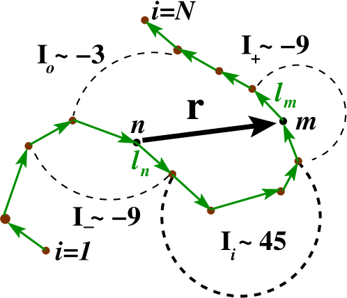
Figure 1: (Color online) Sketch of a polymer chain of length $N$ in a dense melt in $d=3$ dimensions. As notations we use ${\bf r}_{i}$ for the position vector of a monomer $i$, ${\bf l}_{i}={\bf r}_{i+1}-{\bf r}_{i}$ for its bond vector, ${\bf r}={\bf r}_{m}-{\bf r}_{n}$ for the end-to-end vector of the chain segment between the monomers $n$ and $m=n+s$ and $r=||{\bf r}||$ for its length. Segment properties, such as the $2p$-th moments $\left<{\bf r}^{2p}\right>$, are averaged over all possible pairs of monomers $(n,m)$ of a chain and over all chains. The second moment ($p=1$) is denoted $R_{\text{e}}(s)=\left<{\bf r}^{2}\right>^{1/2}$, the total chain end-to-end distance is $R_{\text{e}}(s=N-1)$. The dashed lines show the relevant graphs of the analytical perturbation calculation outlined in Sec. II.2. The numerical factors indicate for infinite chains (without chain end effects) the relative weights contributing to the $1/\sqrt{s}$-swelling of $R_{\text{e}}(s)$ indicated in Eq. (10).

One immediate consequence of Flory’s hypothesis is that the mean-squared size of chain segments of curvilinear length $s=m-n$ (with $1\leq n<m<N$) should scale as $R_{\text{e}}^{2}(s)\equiv\left<{\bf r}^{2}\right>={b_{\text{e}}^{2}s}$ if the two monomers $n$ and $m$ on the same chain are sufficiently separated along the chain backbone, and local correlations may be neglected ($1\ll s$). For the total chain ($s=N-1\gg 1$) this implies obviously that $R_{\text{e}}^{2}(N-1)=b_{\text{e}}^{2}(N-1)\approx b_{\text{e}}^{2}N$. Here, $N$ denotes the number of monomers per chain, ${\bf r}$ the end-to-end vector of the segment, $r=||{\bf r}||$ its length and $b_{\text{e}}$ the “effective bond length” of asymptotically long chains Doi and Edwards (1986). (See Fig. 1 for an illustration of some notations used in this paper.) For the $2p$-th moment ($p=0,1,2,\ldots$) of the segmental size distribution $G(r,s)$ in three dimensions one may write more generally

$$K_{p}(s)\equiv 1-\frac{6^{p}p!}{(2p+1)!}\frac{\left<{\bf r}^{2p}\right>}{(b_{\text{e}}^{2}s)^{p}}=0$$ (1)

which is, obviously, consistent with a Gaussian segmental size distribution

$$G_{0}(r,s)=\left(\frac{3}{2\pi sb_{\text{e}}^{2}}\right)^{3/2}\exp\left(-\frac{3}{2}\frac{r^{2}}{b_{\text{e}}^{2}s}\right).$$ (2)

Both equations are expected to hold as long as the moment is not too high for a given segment length and the finite-extensibility of the polymer strand remains irrelevant Doi and Edwards (1986).

Deviations caused by the segmental correlation hole effect.

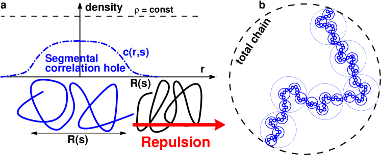
Figure 2: (Color online) Role of incompressibility and chain connectivity in dense polymer solutions and melts. (a) Sketch of the segmental correlation hole of a marked chain segment of curvilinear length $s$. Density fluctuations of chain segments must be correlated, since the total density fluctuations (dashed line) are small. Consequently, a second chain segment feels an entropic repulsion when both correlation holes start to overlap. (b) Self-similar pattern of nested segmental correlation holes of decreasing strength $u(s)\approx s/\rho R(s)^{3}\approx c_{\text{e}}/\sqrt{s}$ aligned along the backbone of a reference chain. The large dashed circle represents the classical correlation hole of the total chain ($s\approx N$) de Gennes (1979). This is the input of recent approaches to model polymer chains as soft spheres Likos (2001); Yatsenko et al. (2004). We argue that incompressibility on all scales and chain connectivity leads to a short distance repulsion of the segmental correlation holes, which increases with decreasing $s$.

Recently, Flory’s hypothesis has been challenged both theoretically Schäfer (1999); Semenov and Johner (2003); Semenov and Obukhov (2005); Beckrich et al. (2007a); Beckrich (2006) and numerically for three-dimensional solutions Schäfer et al. (2000); Auhl et al. (2003); Wittmer et al. (2004); Wittmer et al. (2007a, b) and ultrathin films Cavallo et al. (2005); Meyer et al. (2007). These studies suggest that intra- and interchain excluded volume forces do not fully compensate each other on intermediate length scales, leading to long-range intrachain correlations. The general physical idea behind these correlations is related to the “segmental correlation hole” of a typical chain segment Wittmer et al. (2007a). As sketched in Fig. 2, this induces an effective repulsive interaction when bringing two segments together, and swells (to some extent) the chains causing, hence, a systematic violation of Eq. (1). Elaborating and clarifying various points already presented briefly elsewhere Wittmer et al. (2004); Wittmer et al. (2007a, b), we focus here on melts of long and flexible polymers. Using two well-studied coarse-grained polymer models Baschnagel et al. (2004) various intrachain properties are investigated numerically as functions of $s$ and compared with predictions from first-order perturbation theory. (For a discussion of intrachain correlations in reciprocal space see Refs. Wittmer et al. (2007a); Beckrich et al. (2007a); Beckrich (2006).)

Central results tested in this study.

The key claim verified here concerns the deviation $\delta G(r,s)=G(r,s)-G_{0}(r,s)$ of the segmental size distribution $G(r,s)$ from Gaussianity, Eq. (2), for asymptotically long chains ($N\rightarrow\infty$) in the “scale-free regime” ($1\ll s\ll N$). We show that the relative deviation divided by $c_{\text{e}}/\sqrt{s}$ scales as a function $f(n)$ of $n=r/b_{\text{e}}\sqrt{s}$:

$$\frac{\delta G(r,s)/G_{0}(r,s)}{c_{\text{e}}/\sqrt{s}}=f(n)=\sqrt{\frac{3\pi}{32}}\left(-\frac{2}{n}+9n-\frac{9}{2}n^{3}\right).$$ (3)

As we shall see, this scaling holds indeed for sufficiently large segment size $r$ and curvilinear length $s$. The indicated “swelling coefficient” $c_{\text{e}}$ has been predicted analytically,

$$c_{\text{e}}=\frac{\sqrt{24/\pi^{3}}}{\rho b_{\text{e}}^{3}}$$ (4)

($\rho$ being the monomer number density), where we shall argue that the bond length of the Gaussian reference chain of the perturbation calculation must be renormalized to the effective bond length $b_{\text{e}}$. Accepting Eq. (3) the swelling of the segment size is readily obtained by computing $\left<{\bf r}^{2p}\right>=4\pi\int dr\ r^{2+2p}G(r,s)$. For the $2p$-th moment this yields

$$K_{p}(s)=\frac{3(2^{p}p!p)^{2}}{2(2p+1)!}\ \frac{c_{p}}{\sqrt{s}}.$$ (5)

For instance, for the second moment ($p=1$) this reduces to $K_{1}(s)=1-R_{\text{e}}(s)^{2}/b_{\text{e}}^{2}s=c_{1}/\sqrt{s}\approx c_{\text{e}}/\sqrt{s}$. We have replaced in Eq. (5) the theoretically expected swelling coefficient $c_{\text{e}}$ by empirically determined coefficients $c_{p}$. It will be shown, however, that $c_{p}/c_{\text{e}}$ is close to unity for all moments. Effectively, this reduces Eq. (5) to an efficient one-parameter extrapolation formula for the effective bond length $b_{\text{e}}$ of asymptotically long chains albeit empirical and theoretical swelling coefficients may slightly differ. While we show how $b_{\text{e}}$ may be fitted, no attempt is made to predict it from the operational model parameters and other measured properties such as the microscopic structure or the bulk compression modulus Edwards (1975); Muthukumar and Edwards (1982); Doi and Edwards (1986).

Outline.

We begin our discussion by sketching the central theoretical ideas in Sec. II. There we will give a simple scaling argument and outline very briefly some elements of the standard perturbation calculations we have performed to derive them (Sec. II.2). Details of the analytical treatment are relegated to Appendix A. The numerical models and algorithms allowing the computation of dense melts containing the large chain lengths needed for a clear-cut test are presented in Sec. III. Our computational results are given in Sec. IV. While focusing on long chains in dense melts, we explain also briefly effects of finite chain size. The general background of this work and possible consequences for other problems of polymer science are discussed in the final Sec. V.

II Physical idea and sketch of the perturbation calculation

II.1 Scaling arguments

Incompressibility and correlation of composition fluctuations.

Polymer melts are essentially incompressible on length scales large compared to the monomer diameter, and the density $\rho$ of all monomers does not fluctuate. On the other hand, composition fluctuations of labeled chains or subchains may certainly occur, however, subject to the total density constraint. Composition fluctuations are therefore coupled and segments feel an entropic penalty when their distance becomes comparable to their size Semenov and Johner (2003); Wittmer et al. (2007a). As sketched in Fig. 2(a), we consider two independent test chains of length $s$ in a melt of very long chains ($N\rightarrow\infty$). If $s$ is sufficiently large, their typical size, $R(s)\approx b_{\text{e}}\sqrt{s}$, is set by the effective bond length $b_{\text{e}}$ of the surrounding melt (taking apart finite chain-size effects). The test chains interact with each other directly and through the density fluctuations of the surrounding melt. The scaling of their effective interaction may be obtained from the potential of mean force $U(r,s)\equiv-\ln(g(r,s)/g(\infty,s))$ where $g(r)$ is the probability to find the second chain at a distance $r$ assuming the first segment at the origin ($r=0$). Since the correlation hole is shallow for large $s$, expansion leads to $U(r,s)\approx 1-g(r,s)/g(\infty,s)\approx c(r,s)/\rho$ with $c(r,s)$ being the density distribution of a test chain around its center of mass. This distribution scales as $c(r\approx 0,s)\approx s/R(s)^{d}$ close to the center of mass ($d$ being the dimension of space) and decays rapidly at distances of order $R(s)$ de Gennes (1979). Hence, the interaction strength at $r/R(s)\ll 1$ is set by $u(s)\equiv U(0,s)\equiv c(0,s)/\rho\approx s/\rho R(s)^{d}\sim s^{1-d/2}$ Semenov and Johner (2003); Wittmer et al. (2007a). Interestingly, $u(s)$ does not depend explicitly on the bulk compression modulus $v$. It is dimensionless and independent of the definition of the monomer unit, i.e. it does not change if $\lambda$ monomers are regrouped to form an effective monomer ($\rho\to\rho/\lambda$, $s\to s/\lambda$) while keeping the segment size $R$ fixed.

Connectivity and swelling.

To connect both test chains to form a chain of length $2s$ the effective energy $u(s)$ has to be paid and this repulsion will push the half-segments apart. We consider next a segment of length $s$ in the middle of a very long chain. All interactions between the test segment and the rest of the chain are first switched off but we keep all other interactions, especially within the segment and between the segment monomers and monomers of surrounding chains. The typical size $R(s)$ of the test segment remains essentially unchanged from the size of an independent chain of same strand length. If we now switch on the interactions between the segment and monomers on adjacent segments of same length $s$, this corresponds to an effective interaction of order $u(s)$ as before. (The effect of switching on the interaction to all other monomers of the chain is inessential at scaling level, since these other monomers are more distant.) Since this repels the respective segments from each other, the corresponding subchain is swollen compared to a Gaussian chain of non-interacting segments. It is this effect we want to characterize.

Perturbation approach in three dimensions.

In the following we will exclusively consider chain segments $s$ which are much larger than the number of monomers $g\equiv 1/v\rho$ contained in a blob de Gennes (1979), i.e. we will look on a scale where incompressibility matters. (The number $g$ is also sometimes called “dimensionless compressibility” Beckrich et al. (2007a).) Interestingly, when taken at $s=g$ the interaction strength takes the value

$$u(s=g)\approx\frac{g}{\rho b_{\text{e}}^{d}g^{d/2}}=\frac{(v\rho)^{d/2-1}}{\rho b_{\text{e}}^{d}}\approx G_{\text{z}}$$ (6)

with $G_{\text{z}}$ being the standard Ginzburg parameter used for the perturbation calculation of strongly interacting polymers Doi and Edwards (1986). Hence, the segmental correlation hole potential $u(s)\approx G_{\text{z}}(g/s)^{d/2-1}\ll G_{\text{z}}$ for $d>2$ and $s\gg g$. Although for real polymer melts as for computational systems large values of $G_{\text{z}}\approx 1$ may sometimes be found, $u(s)\sim 1/\sqrt{s}$ decreases rapidly with $s$ in three dimensions, as illustrated in Fig. 2(b), and standard perturbation calculations can be successfully performed.

As sketched in the next paragraph these calculations yield quantities $K[u]$ which are defined such that they vanish ($K[u=0]=0$) if the perturbation potential $u(s)$ is switched off and are then shown to scale, to leading order, linearly with $u$. For instance, for the quantity $K_{p}(s)$, defined in Eq. (1), characterizing the deviation of the chain segment size from Flory’s hypothesis one thus expects the scaling

$$K_{p}[u(s)]\approx+u(s)\approx+\frac{s}{\rho R^{d}(s)}.$$ (7)

The $+$-sign indicated marks the fact that the prefactor has to be positive to be consistent with the expected swelling of the chains. Consequently, the typical segment size, $R(s)/b_{\text{e}}\sqrt{s}\approx 1-u(s)$, must approach the asymptotic limit for large $s$ from below. For three dimensional solutions Eq. (7) implies that $K_{p}(s)$ should vanish rapidly as $1/(\rho b_{\text{e}}^{3}\sqrt{s})$. (This is different in thin films where $u(s)\approx G_{\text{z}}$ decays only logarithmically Semenov and Johner (2003) as may be seen from Eq. (33) given below.) Taking apart the prefactors — which require a full calculation — this corresponds exactly to Eq. (5) with a swelling coefficient $c_{\text{e}}\approx c_{p}\approx 1/\rho b_{\text{e}}^{3}$ in agreement with Eq. (4). Note also that the predicted deviations are inversely proportional to $b_{\text{e}}^{3}$, i.e. the more flexible the chains, the more pronounced the effect. Similar relations $K[u]\sim u$ may also be formulated for other quantities and will be tested numerically in Sec. IV. There, we will also check that the linear order is sufficient.

II.2 Perturbation calculation

Generalities.

Before delving more into our computational results we summarize here how Eqs. (3-5) and related relations have been obtained using standard one-loop perturbation calculation. The general task is to determine $\left<\mbox{$\cal A$}\right>\approx\left<\mbox{$\cal A$}\right>_{0}(1+\left<U\right>_{0})-\left<\mbox{$\cal A$}U\right>_{0}$ for measurable quantities $\cal A$ such as the squared distance between two monomers $n$ and $m$ on the same chain, $\mbox{$\cal A$}={\bf r}_{nm}^{2}$. Here, $\left<...\right>_{0}$ denotes the average over the distribution function of the unperturbed ideal chain of bond length $b$ and $U=\int_{0}^{N}dk\,\int_{0}^{k}dl\,\tilde{v}(r_{kl})$ the effective perturbation potential. We discuss first the general results in the scale free regime ($1\ll s\ll N$), argue then that $b$ should be renormalized to the effective bond length $b_{\text{e}}$ and sketch finally the calculation of finite chain-size effects.

The scale free regime.

Following Edwards Edwards (1965, 1966); Doi and Edwards (1986), the Gaussian (or “Random Phase” de Gennes (1979)) approximation of the pair interaction potential in real space is

$$\tilde{v}(r)=v\ \left(\delta(r)-\frac{\exp(-r/\xi)}{4\pi r\xi^{2}}\right)$$ (8)

where $v$ is a parameter which tunes the monomer interaction. (It is commonly associated with the bare excluded volume of the monomers Doi and Edwards (1986), but should more correctly be identified with the bulk modulus effectively measured for the system. See the discussion of Eq. (15) of Ref. (Semenov and Obukhov (2005)).) The effective potential consists of a strongly repulsive part $v\delta(r)$ of very short range, and a weak attractive part of range $\xi$ where the correlation length of the density fluctuations is given by $\xi^{2}=b^{2}g/12$ with $g=1/\rho v$. In Fourier space Eq. (8) is equivalent to

$$\tilde{v}(q)=v\ \frac{q^{2}}{q^{2}+\xi^{-2}}$$ (9)

with $q$ being the wave vector. This is sufficient for calculating the scale free regime corresponding to asymptotically long chains where chain end effects may be ignored. The different graphs one has to compute are indicated in Fig. 1. For $\mbox{$\cal A$}={\bf r}^{2}$ (with $1\ll n<m\ll N$) this yields, e.g.,

$$\left<{\bf r}^{2}\right> = b^{2}\left(1+\frac{12}{\pi}\frac{v\xi}{b^{4}}\right)(m-n)-\frac{\sqrt{24/\pi^{3}}}{\rho b}\sqrt{m-n}$$ (10)

$$= b_{\text{e}}^{2}s\left(1-\frac{c_{\text{e}}}{\sqrt{s}}\left(\frac{b_{\text{e}}}{b}\right)\right).$$

In the second line we have used the definition of the swelling coefficient $c_{\text{e}}$ indicated in Eq. (4) and have set

$$b_{\text{e}}^{2}\equiv b^{2}\left(1+p\frac{12}{\pi}\frac{v\xi}{b^{4}}\right)=b^{2}\left(1+p\frac{\sqrt{12}}{\pi}G_{\text{z}}\right)$$ (11)

with $G_{\text{z}}\equiv\sqrt{v\rho}/b^{3}\rho$ and $p=1$. (The prefactor $p$ has been added for convenience.) The coefficient $b_{\text{e}}$ of the leading Gaussian term in Eq. (10) — entirely due to the graph $I_{i}$ describing the interactions of monomers inside the segment between $n$ and $m$ — has been predicted long ago by Edwards Doi and Edwards (1986). It describes how the effective bond length is increased from $b$ to $b_{\text{e}}$ under the influence of a small excluded volume interaction. The second term in Eq. (10) entails the $1/\sqrt{s}$-swelling which is investigated numerically in this paper. It does only depend on $b$ and $\rho$ but, more importantly, not on $v$ — in agreement with the scaling of $u(s)$ discussed in Sec. II.1. The relative weights contributing to this term are indicated in Fig. 1 in units of $-\sqrt{6/\pi^{3}}v\xi^{2}/b^{3}\sqrt{s}$. The diagrams $I_{-}$ and $I_{+}$ are obviously identical in the scale free limit. Note that the interactions described by the strongest graph $I_{i}$ align the bonds ${\bf l}_{n}$ and ${\bf l}_{m}$ while the others tend to reduce the effect.

For higher moments of the segment size distribution $G(r,s)$ it is convenient to calculate first the deviation of the Fourier-Laplace transformation of $\delta G(r,s)$ and to obtain the moments from the coefficients of the expansion of this “generating function” in terms of the squared wave vector $q^{2}$. As explained in detail in the Appendix A this yields more generally

$$\left<{\bf r}^{2p}\right>=\frac{(2p+1)!}{6^{p}p!}(b_{\text{e}}^{2}s)^{p}\left(1-\frac{3(2^{p}p!p)^{2}}{2(2p+1)!}\frac{c_{\text{e}}}{\sqrt{s}}\ \left(\frac{b}{b_{\text{e}}}\right)^{2p-3}\right)$$ (12)

where we have used Eq. (11) with general $p$. Obviously, Eq. (12) is consistent with our previous finding Eq. (10) for $p=1$. The corresponding segmental size distribution is

$$G(r,s) = \left(\frac{3}{2\pi b_{\text{e}}^{2}s}\right)^{3/2}\exp\left(-\frac{3}{2}\frac{r^{2}}{b_{\text{e}}^{2}s}\right)$$ (13)

$$+ \left(\frac{3}{2\pi b^{2}s}\right)^{3/2}\exp\left(-\frac{3}{2}\frac{r^{2}}{b^{2}s}\right)\frac{c_{\text{e}}}{\sqrt{s}}\left(\frac{b_{\text{e}}}{b}\right)^{3}f(n)$$

with $n=r/b\sqrt{s}$ and $f(n)$ being the same function as indicated in Eq. (3). The leading Gaussian terms in Eqs. (12) and (13) depend on the effective bond length $b_{\text{e}}$, the second only on the Kuhn length $b$ of the reference chain. When comparing these result with Eqs. (3) and (5) proposed in the Introduction, one sees that both equations are essentially identical — taken apart, however, that they depend on $b$ and $b_{\text{e}}$. Note the conspicuous factor $(b/b_{\text{e}})^{2p-3}$ in Eq. (12) which would strongly reduce the empirical swelling coefficients $c_{p}=c_{\text{e}}(b/b_{\text{e}})^{2p-3}$ for large $p$ if $b$ and $b_{\text{e}}$ were different.

Interpretation of first-loop results in different contexts.

The above perturbation results may be used directly to describe the effect of a weak excluded volume $v$ on a reference system of perfectly ideal polymer melts with Kuhn segment length $b$ where all interactions have been switched off ($v=0$). It is expected to give a good estimation for the effective bond length $b_{\text{e}}$ only for a small Ginzburg parameter: $G_{\text{z}}\ll 1$. For the dense melts we want to describe this does not hold (Sec. III) and one cannot hope to find a good quantitative agreement with Eq. (11). Note also that large wave vectors contribute strongly to the leading Gaussian term. The effective bond length $b_{\text{e}}$ is, hence, strongly influenced by local and non-universal effects and is very difficult to predict in general.

Our much more modest goal is to predict the coefficient of the $1/\sqrt{s}$-perturbation and to express it in terms of a suitable variational reference Hamiltonian characterized by a conveniently chosen Kuhn segment $b$ and the measured effective bond length $b_{\text{e}}$ (instead of Eq. (11)). Following Muthukumar and Edwards Muthukumar and Edwards (1982), we argue that for dense melts $b$ should be renormalized to $b_{\text{e}}$ to take into account higher order graphs. No strict mathematical proof can be given at present that the infinite number of possible graphs must add up in this manner. Our hypothesis relies on three observations:

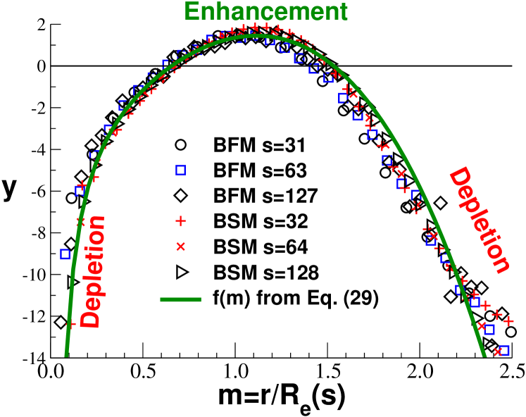
Figure 13: (Color online) Replot of the relative deviation of the measured segment size distribution, $y=(\delta G(r,s)/G_{0}(r,s)))/(c_{\text{e}}/\sqrt{s})$, as a function of $m=r/R_{\text{e}}(s)$. The figure highlights that the measured segment size is the only length scale relevant for describing the deviation from Flory’s hypothesis. The same data sets and symbols are used as in the previous Fig. 12.

• The general scaling argument discussed in Sec. II.1 states that we have only one relevant length scale in this problem, the typical segment size $R(s)\approx b_{\text{e}}\sqrt{s}$ itself. The incompressibility constraint cannot generate an additional scale. It is this size $R(s)$ which sets the strength of the effective interaction which then in turn feeds back to the deviations of $R(s)$ from Gaussianity. Having a bond length $b$ in addition to the effective bond length $b_{\text{e}}$ associated with $R(s)$ would imply incorrectly a second length scale $b\sqrt{s}$ varying independently with the bulk modulus $v$. (We will check explicitly below in Fig. 13 that there is only one length scale.) This implies $b/b_{\text{e}}=\mbox{const}\ v^{0}$.

• Thus, since by construction $b/b_{\text{e}}=1$ for $v\rightarrow 0$, it follows that both lengths should be equal for all $v$.

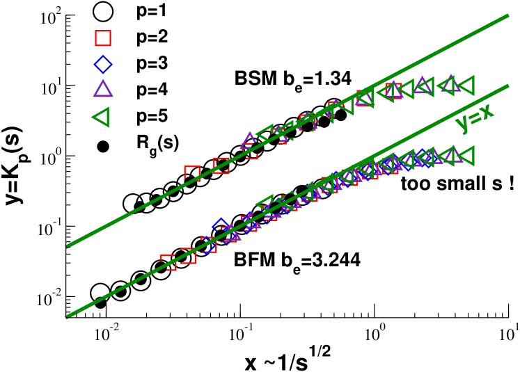
Figure 6: (Color online) Critial test of Eq. (5) where the rescaled moments $y=K_{p}(s)$ of the segment size distribution (defined in Eq. (1)) are plotted vs. $x=\frac{3(2^{p}p!p)^{2}}{2(2p+1)!}\ \frac{c_{p}}{\sqrt{s}}$. We consider the first five even moments ($p=1,\ldots,5$) for the BFM with $N=2048$ and the BSM with $N=1024$. Also indicated is the rescaled radius of gyration, $y=5/8\ (1-6R_{\text{g}}^{2}(s)/b_{\text{e}}^{2}(s+1))$, as a function of $x=c_{1}/\sqrt{s+1}$ (filled circles). The BSM data has been shifted upwards for clarity. Without this shift a perfect data collapse is found for both models and all moments. Keeping the same effective bond length $b_{\text{e}}$ for all moments of each model we fit for the swelling coefficients $c_{p}$ by rescaling the horizontal axis. We find $b_{\text{e}}\approx 3.244$ for the BFM and $1.34$ for the BSM. If $b_{\text{e}}$ is chosen correctly, all data sets extrapolate linearly to zero for large $s$ ($x\rightarrow 0$). The swelling coefficients found are close the theoretical prediction $c_{\text{e}}$, as indicated in Tab. 2. The plot demonstrates that the non-Gaussian deviations scale as the segmental correlation hole, $u(s)\sim c_{\text{e}}/\sqrt{s}$ and this for all moments as long as $x\ll 1$. The saturation at large $x$ is due to the finite extensibility of short chain segments. Since this effect becomes more marked for larger moments, the fit of $b_{\text{e}}$ is best performed for $p=1$.

• We know from Eq. (12) that the empirical coefficients $c_{p}=c_{\text{e}}(b/b_{\text{e}})^{2p-3}$ should depend strongly on the moment considered if the ratio $b/b_{\text{e}}$ is not close to unity. It will be shown below (Fig. 6) that $c_{p}/c_{\text{e}}\approx 1$ for all $p$. This implies $b\approx b_{\text{e}}$.

Finite chain size effects.

To describe properly finite chain size corrections Eq. (9) must be replaced by the general linear response formula

$$\frac{1}{\tilde{v}(q)}=\frac{1}{v}+\rho F(q)$$ (14)

with $F(q)=Nf_{D}(x)$ being the form factor of the Gaussian reference chain given by Debye’s function $f_{D}(x)=2(e^{-x}-1+x)/x^{2}$ with $x=(qb)^{2}N/6$ Doi and Edwards (1986). This approximation allows in principle to compute, for instance, the (mean-squared) total chain end-to-end distance, $\mbox{$\cal A$}=({\bf r}_{N}-{\bf r}_{1})^{2}$. One verifies readily (see Doi and Edwards (1986), Eq. (5.III.9)) that the effect of the perturbation may be expressed as

$$\left<\mbox{$\cal A$}\right>_{0}\left<U\right>_{0}-\left<\mbox{$\cal A$}U\right>_{0}=\int\frac{d^{3}\bf{q}}{(2\pi)^{3}}\ \tilde{v}(q)\ \frac{q^{2}b^{4}}{9}\int_{0}^{N}ds\ s^{2}(N-s)\exp\left(-\frac{q^{2}b^{2}s}{6}\right).$$ (15)

We take now first the integral over $s$. In the remaining integral over $q$ small $q$ wave vectors contribute to the $\sqrt{N}$-swelling while large $q$ renormalize the effective bond length of the dominant Gaussian behaviour linear in $N$ (as discussed above). Since we wish to determine the non-Gaussian corrections, we may focus on small wave vectors $q\ll 1/\xi$. Since in this limit $1/v=\rho g\ll\rho F(q)$, one can neglect in Eq. (14) the $1/v$ contribution to the inverse effective interaction potential. We thus continue the calculation using the much simpler $\tilde{v}(N,x)=1/(N\rho f_{D}(x))$. This allows us to express the swelling as

$$1-\frac{\left<({\bf r}_{N}-{\bf r}_{1})^{2}\right>}{b_{\text{e}}^{2}N}=\frac{c_{\text{e}}}{\sqrt{N}}\ I(x_{u}).$$ (16)

To simplify the notation we have set here finally $b=b_{\text{e}}$ in agreement with the hypothesis discussed above. The numerical integral $I(x_{u})=\int_{0}^{x_{u}}dx\ldots$ over $x$ is slowly convergent at infinity. As a consequence the estimate $I(\infty)=1.59$ may be too large for moderate chain lengths. In practice, convergence is not achieved for values $x_{u}(N)\approx(b/\xi)^{2}N$ corresponding to the screening length $\xi$.

We remark finally that numerical integration can be avoided for various properties if the Padé approximation of the form factor, $F(q)=N/(1+(qb)^{2}N/12)$, is used. This allows analytical calculations by means of the simplified effective interaction potential

$$\tilde{v}(q)=\frac{q^{2}b^{5}}{12\rho b^{3}}+\frac{b^{3}}{N\rho b^{3}}.$$ (17)

This has been used for instance for the calculation of finite chain size effects for the bond-bond correlation function discussed in Sec. IV.3 below .

III Computational models and technical details

III.1 Bond fluctuation model

A widely-used lattice Monte Carlo scheme for coarse-grained polymers.

The body of our numerical data comes from the three dimensional bond fluctuation model (BFM) — a lattice Monte Carlo (MC) algorithm where each monomer occupies eight sites of a unit cell of a simple cubic lattice Carmesin and Kremer (1988); Deutsch and Binder (1991); Paul et al. (1991). Our version of the BFM with $108$ bond vectors corresponds to flexible athermal chain configurations Baschnagel et al. (2004). All length scales are given in units of the lattice constant and time in units of Monte Carlo Steps (MCS). We use cubic periodic simulation boxes of linear size $L=256$ containing $n_{\text{mon}}=\rho L^{3}=2^{20}\approx 10^{6}$ monomers. This monomer number corresponds to a monomer number density $\rho=0.5/8$ where half of the lattice sites are occupied (volume fraction $0.5$). The large system sizes used allow us to suppress finite box-size effects for systems with large chains. Using a mix of local, slithering snake Kron (1965); Wall and Mandel (1975); Mattioni et al. (2003), and double-bridging Karayiannis et al. (2002); Banaszak and de Pablo (2003); Auhl et al. (2003); Baschnagel et al. (2004) MC moves we were able to equilibrate dense systems with chain lengths up to $N=8192$.

Equilibration and sampling of high-molecular BFM melts.

Standard BFM implementations Paul et al. (1991); Müller et al. (2000); Kreer et al. (2001) use local MC jumps to the 6 closest lattice sites to prevent the crossing of chains and conserve therefore the chain topology. These “L06” moves lead to very large relaxation times, scaling at least as $\tau_{\text{e}}\sim N^{3}$, as may be seen from Fig. 3 (stars). The relaxation time $\tau_{\text{e}}=R_{\text{e}}^{2}/6D_{\text{s}}$ indicated in this figure has been estimated from the self-diffusion coefficient $D_{\text{s}}$ obtained from the mean-square displacements of all monomers in the free diffusion limit. (For the largest chain indicated for L06 dynamics only a lower bound for $\tau_{\text{e}}$ is given.) Instead of this more realistic but very slow dynamical scheme we make jump attempts to the 26 sites of the cube surrounding the current monomer position (called “L26” moves). This allows the chains to cross each other which dramatically speeds up the dynamics, especially for long chains ($N>512$). If only local moves are considered, the dynamics is perfectly consistent with the Rouse model Doi and Edwards (1986). As shown in Fig. 3, we find $\tau_{\text{e}}\approx 530N^{2}$ for L26 dynamics. This is, however, still prohibitive by large for sampling configurations with the longest chain length $N$ we aim to characterize .

Slithering snake moves.

In addition to the local moves one slithering snake move per chain is attempted on average per MCS corresponding to the displacement of $N$ monomer along the chain backbone. Note that in our units two spatial displacement attempts per MCS are performed on average per monomer, one for a local move and one for a snake move. (In practice, it is computationally more efficient for large $N$ to take off a monomer at one chain end and to paste it at the other leaving all other monomers unaltered. Before dynamical measurements are performed the original order of beads must then be restored.) Interestingly, a significantly larger slithering snake attempt frequency would not be useful since the relaxation time of slithering snakes without or only few local moves increases exponentially with mass Deutsch (1985); Mattioni et al. (2003) due to the correlated motion of snakes Semenov (1997). In order to obtain an efficient free snake diffusion (with a chain length independent curvilinear diffusion coefficient $D_{\text{c}}(N)\sim N^{0}$ and $\tau_{\text{e}}\approx N^{2}/D_{\text{c}}(N)\sim N^{2}$ Wall and Mandel (1975); Mattioni et al. (2003)) it is important to relax density fluctuations rapidly by local dynamical pathways. As shown in Fig. 3 (squares), we find a much reduced relaxation time $\tau_{\text{e}}\approx 40N^{2}$ which is, however, still unconveniently large for our longest chains. Note that most of the CPU time is still used by local moves. The computational load per MCS remains therefore essentially chain length independent.

Advantages and pitfalls of double-bridging moves.

Double-bridging (DB) moves are very useful for high densities and help us to extend the accessible molecular masses close to $10^{4}$. As for slithering snake moves we use all $108$ bond vectors to switch chain segments between two different chains. Only chain segments of equal length are swapped to conserve monodispersity. Topolocial constraints are again systematically and deliberately violated. Since more than one swap partner is possible for a selected first monomer, delicate detailed balance questions arise. This is particularly important for short chains and is discussed in detail in Ref. Baschnagel et al. (2004). Technically, the simplest solution to this problem is to refuse all moves with more than one swap partner (to be checked both for forward and back move). The configurations are screened with a frequency $f_{\text{DB}}$ for possible DB moves where we scan in random order over the monomers. The frequency should not be too large to avoid (more or less) immediate back swaps and monomers should move at least out of the local monomer cage and over a couple of lattice sites. We use $f_{\text{DB}}=0.1$ between DB updates for the configurations reported here. (The influence of $f_{\text{DB}}$ on the performance has not been explored systematically, but preliminary results suggest a slightly smaller DB frequency for future studies.) The diffusion times over the end-to-end distance for this case are indicated in Tab. 1. As shown in Fig. 3, we find empirically $\tau_{\text{e}}(N)\approx 13N^{1.62}$. For $N=8192$ this corresponds to $3\cdot 10^{7}$ MCS. This allows us even for the largest chain lengths to observe monomer diffusion over several $R_{\text{e}}$ within the $10^{8}$ MCS which are feasible on our XEON-PC processor cluster.

The efficiency of DB moves is commonly characterized in terms of the relaxation time $\tau_{\text{ee}}$ of the end-to-end vector correlation function Karayiannis et al. (2002); Banaszak and de Pablo (2003). For normal chain dynamics this would indeed characterize the longest relaxation time of the system, i.e. $\tau_{\text{e}}\approx\tau_{\text{ee}}$. For the double-bridging this is, however, not sufficient since density fluctuations do not couple to the bridging moves and can not be relaxed. We find therefore that configurations equilibrate on time scales given by $\tau_{\text{e}}$ rather than by $\tau_{\text{ee}}\ll\tau_{\text{e}}$. This may be verified, for instance, from the time needed for the distribution $R_{\text{e}}(s)$ (and especially its spatial components) to equilibrate. The criterion given in the literature Karayiannis et al. (2002) is clearly not satisfactory and may lead to insufficiently equilibrated configurations. In summary, equilibration with DB moves still requires monomer diffusion over the typical chain size, however at a much reduced price.

Some properties of our configurations.

The Tables 1 and 2 summarize some system properties obtained for our reference density $\rho=0.5/8$. Averages are performed over all chains and $1000$ configurations. These configurations may be considered to be independent for $N<4096$. Only a few independent configurations exist for the largest chain length $N=8192$ which has to be considered with some care. Taking apart this system, chains are always much smaller than the box size. For asymptotically long chains, we obtain an average bond length $\left<|{\bf l}|\right>\approx 2.604$, a root-mean-squared bond length $l\equiv\left<{\bf l}^{2}\right>^{1/2}\approx 2.635$ and an effective bond length $b_{\text{e}}\approx 3.244$ — as we will determine below in Sec. IV.1. This corresponds to a ratio $C_{\infty}\equiv b_{\text{e}}^{2}/l^{2}\approx 1.52$ and, hence, to a persistence length $l_{\text{p}}=l(C_{\infty}+1)/2\approx 3.32$ Baschnagel et al. (2004). Especially, we find from the zero wave vector limit of the total structure factor $S(q)$ a low (dimensionless) compressibility $g=S(q\rightarrow 0)/\rho\approx 0.246$ which compares well with real experimental melts. From the measured bulk compression modulus $v\equiv 1/g(\rho)\rho$ and the effective bond length $b_{\text{e}}$ one may estimate a Ginzburg parameter $G_{\text{z}}=\sqrt{v\rho}/b_{\text{e}}^{3}\rho\approx 0.96$. Following Ref. Semenov and Obukhov (2005) the interaction parameter $v$ is supposed here to be given by the full inverse compressibility and not just by the second virial coefficient.

III.2 Bead spring model

Hamiltonian.

Additionally, molecular dynamics simulations of a bead-spring model (BSM) Meyer and Müller-Plathe (2001) were performed to dispel concerns that our results are influenced by the underlying lattice structure of the BFM. The model is derived from a coarse-grained model for polyvinylalcohol which has been employed to study polymer crystallization Meyer and Müller-Plathe (2002). It is characterized by two potentials: a non-bonded potential of Lennard-Jones (LJ) type and a harmonic bond potential. While the often employed Kremer-Grest model Kremer and Grest (1990) uses a $12-6$ LJ potential to describe the non-bonded interactions $U_{\text{nb}}(r)$, our non-bonded potential has a softer repulsive part. It is given by

$$U_{\text{nb}}(r)=1.511\left[\left(\frac{\sigma_{0}}{r}\right)^{9}-\left(\frac{\sigma_{0}}{r}\right)^{6}\right],$$ (18)

which is truncated and shifted at the minimum at $r_{\text{min}}\approx 1.15$. Note that all length scales are given in units of $\sigma_{0}$ and we use LJ units Allen and Tildesley (1994) for all BSM data (mass $m=1$, Boltzmann constant $k_{\text{B}}=1$). The parameters of the bond potential, $U_{\text{b}}(r)=1120(r-l_{\text{b}})^{2}$, are adjusted so that the average bond length $l(\rho=0.84)\approx l_{\text{b}}=0.97$ is approximately the same as in the standard Kremer-Grest model Kremer and Grest (1990). The average bond length and the root-mean-squared bond length are almost identical for the BSM due to the very stiff bond potential. Since $r_{\text{min}}/l\approx 1.16$ bonded monomers penetrate each other significantly.

Equilibration and sampling.

We perform standard molecular dynamics simulations in the canonical ensemble with a Langevin thermostat (friction constant $\Gamma=0.5$) at temperature $T=1$. The equations of motion are integrated by the velocity-Verlet algorithm Allen and Tildesley (1994). To improve the statistics for large chain length, we have implemented additional double-bridging moves. Since only few of these MC moves are accepted per unit time, this does affect neither the stability nor the accuracy of the molecular dynamics sweeps.

Some properties obtained.

For clarity, we show only data for chain length $N=1024$ and number density $\rho=0.84$, the typical melt density of the Kremer-Grest model Kremer and Grest (1990). For the reported data we use periodic simulation boxes of linear size $L\approx 62$ containing $n_{\text{mon}}=196608$ monomers, but we have also sampled different boxes sizes (up to $L=77.5$) to check for finite box-size effects. For the reference density a dimensionless compressibility $g\approx 0.08$ is found which is about three times smaller than for our BFM melt. For the effective bond length we obtain $b_{\text{e}}\approx 1.34$, i.e. BSM chains ($C_{\infty}\approx 1.91$, $l_{\text{p}}\approx 1.41$) are slightly stiffer than the corresponding BFM polymers. Fortunately, the product $\rho b_{\text{e}}^{3}\approx 2$ is roughly similar in both models and one expects from Eq. (4) a similar swelling for large $s$. Note finally that the Ginzburg parameter $G_{\text{z}}\approx 1.8$ is much larger than for the BFM systems. As we have emphasized in Sec. II, this should, however, not influence the validity of the perturbation prediction of the expected $1/\sqrt{s}$-swelling of the chains when expressed in terms of the measured effective bond length.

IV Numerical results

As illustrated in Fig. 1, a chain segment of curvilinear length $s>0$ is identified by two monomers $n$ and $m=n+s$ on the same chain. We compute here various moments of chain segment properties where we ensemble-average over all chains and all start points $n$. The statistical accuracy must therefore always decrease for large $s$. We concentrate first on the second moment ($p=1$) of the segmental size distribution. Higher moments and the segmental size distribution are discussed in Sec. IV.5.

IV.1 The swelling of chain segments

Scale free regime for $1\ll s\ll N$.

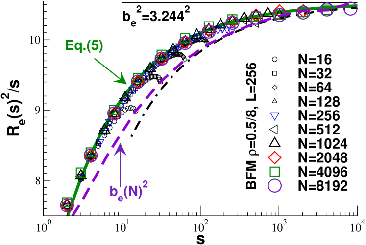
Figure 4: (Color online) Mean-squared segment size $R_{\text{e}}(s)^{2}/s$ vs. curvilinear distance $s$. We present BFM data for different chain length $N$ at number density $\rho=0.5/8$. The averages are taken over all possible monomer pairs $(n,m=n+s)$. The statistics deteriorates, hence, for large $s$. Log-linear coordinates are used to emphasize the power law swelling over several orders of magnitude of $s$. The data approach the asymptotic limit (horizontal line) from below, i.e. the chains are swollen. This behavior is well fitted by Eq. (5) for $1\ll s\ll N$ (bold line). Non-monotonic behavior is found for $s\rightarrow N$, especially for small $N$. The dashed line indicates the measured total chain end-to-end distances, $b_{\text{e}}(N)^{2}\equiv R_{\text{e}}(N-1)^{2}/(N-1)$ from Tab. 1, showing even more pronounced deviations from the asymptotic limit. The dash-dotted line compares this data with Eq. (19).

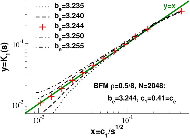
Figure 5: (Color online) Replot of the mean-squared segment size as $y=K_{1}(s)=1-R_{\text{e}}(s)^{2}/b_{\text{e}}^{2}s$ vs. $x=c_{1}/\sqrt{s}$, as suggested by Eq. (5), for different trial effective bond lengths $b_{\text{e}}$ as indicated. Only BFM chains of length $N=2048$ are considered for clarity. This procedure is very sensitive to the value chosen and allows for a precise determination. It assumes, however, that higher order terms in the expansion of $K_{1}(s)$ may be neglected. The value $b_{\text{e}}$ is confirmed from a similar test for higher moments (Fig. 6).

The mean-squared segment size $R_{\text{e}}^{2}(s)=\left<{\bf r}^{2}\right>$ is presented in the Figs. 4, 5 and 6. The first plot shows clearly that chain segments are swollen, i.e. $R_{\text{e}}^{2}(s)/s$ increases systematically and this up to very large curvilinear distances $s$. Only BFM data are shown for clarity. A similar plots exists for the BSM data. In agreement with Eq. (5) for $p=1$, the asymptotic Gaussian behavior (dashed line) is approached from below and the deviation decays as $u(s)\propto 1/\sqrt{s}$ (bold line). The bold line indicated corresponds to $b_{\text{e}}=3.244$ and $c_{1}\approx c_{\text{e}}\approx 0.41$ which fits nicely the data over several decades in $s$ — provided that chain end effects can be neglected ($s\ll N$). Note that a systematic underestimation of the true effective bond length would be obtained by taking simply the largest $R_{\text{e}}^{2}(s)/s\approx 3.23^{2}$ value available, say, for monodisperse chains of length $N=2048$.

Finite chain-size effects.

Interestingly, $R_{\text{e}}^{2}(s)/s$ does not approach the asymptotic limit monotonicly. Especially for short chains one finds a non-monotonic behavior for $s\rightarrow N$. This means that the total chain end-to-end distance $R_{\text{e}}(s=N-1)$ must show even more pronounced deviations from the asymptotic limit. This is confirmed by the dashed line representing the $b_{\text{e}}^{2}(N)\equiv R_{\text{e}}^{2}(N-1)/(N-1)$ data points given in Tab. 1. We emphasize that the non-monotonicity of $R_{\text{e}}^{2}(s)/s$ becomes weaker with increasing $N$ and that, as one expects, the inner distances, as well as the total chain size, are characterized by the same effective bond length $b_{\text{e}}$ for large $s$ or $N$. The non-monotonic behavior may be qualitatively understood by the reduced self-interactions at chain ends which lessens the swelling on these scales. These finite-$N$ corrections have been calculated analytically using the full Debye function for the effective interaction potential $\tilde{v}(q)$, Eq. (14). The prediction for the total chain end-to-end vector given in Eq. (16) is indicated in Fig. 4 (dash-dotted line) where we have replaced the weakly $N$-dependent integral $I(x_{u})$ by its upper bound value for infinite chains

$$1-\frac{R_{\text{e}}^{2}(N-1)}{b_{\text{e}}^{2}\ (N-1)}=\frac{1.59c_{\text{e}}}{\sqrt{N-1}}.$$ (19)

We have changed here the chain length $N$ in the analytical formula (obtained for large chains where $N\approx N-1$) to the curvilinear length $N-1$. This is physically reasonable and allows to take better into account the behavior of small chains. Note that Eq. (19) is similar to Eq. (5) — apart from a slightly larger prefactor explaining the observed stronger deviations. Theory compares well with the measured data for large $N$. It does less so for smaller $N$, as expected, where the chain length dependence of the numerical integral $I(x_{u}(N))\leq 1.59$ must become visible. This explains why the data points are above the dash-dotted line. Note also that additional non-universal finite-$N$ effects not accounted for by the theory are likely for small $N$. In contrast to this, $R_{\text{e}}(s)$ is well described by the theory even for rather small $s$ provided that $N$ is large and chain end effects can be neglected. In summary, it is clear that one should use the segment size $R_{\text{e}}(s)$ rather than the total chain size to obtain in a computational study a reliable fit of the effective bond length $b_{\text{e}}$.

Extrapolation of the effective bond length of asymptotically long chains.

The representation chosen in Fig. 4 is not the most convenient one for an accurate determination of $b_{\text{e}}$ and $c_{1}$. How precise coefficients may be obtained according to Eq. (5) is addressed in the Figs. 5 and 6. The fitting of the effective bond length $b_{\text{e}}$ and its accuracy is illustrated in Fig. 5 for BFM chains of length $N=2048$. This may be first done approximately in linear coordinates by plotting $R_{\text{e}}^{2}(s)/s$ as a function of $1/\sqrt{s}$ (not shown). Since data for large $s$ are less visible in this representation, we recommend for the fine-tuning of $b_{\text{e}}$ to switch then to logarithmic coordinates with a vertical axis $y=1-R_{\text{e}}^{2}(s)/b_{\text{e}}^{2}s$ for different trial values of $b_{\text{e}}$. The correct value of $b_{\text{e}}$ is found by adjusting the vertical axis $y$ such that the data extrapolates linearly as a function of $1/\sqrt{s}$ to zero for large $s$. We assume for the fine-tuning that higher order perturbation corrections may be neglected, i.e. we take Eq. (5) literally. (We show below that higher order corrections must indeed be very small.) The plot shows that this method is very sensitive, yielding a best value that agrees with the theory over more than one order of magnitude without curvature. As expected, it is not possible to rationalize the numerically obtained values $b_{\text{e}}\approx 3.244$ for the BFM and $b_{\text{e}}\approx 1.34$ for the BSM using Eq. (11). According to Eq. (4) these fit values imply the theoretical swelling coefficients $c_{\text{e}}=0.41$ for the BFM and $c_{\text{e}}=0.44$ for the BSM.

Empirical swelling coefficients.

As a next step the horizontal axis is rescaled such that all data sets collapse on the bisection line, i.e. using Eq. (5) we fit for the empirical swelling coefficient $c_{1}$ and compare it to the predicted value $c_{\text{e}}$. This rescaling of the axes allows to compare both models in Fig. 6. For clarity the BSM data have been shifted upwards. For the BFM we find $c_{1}/c_{\text{e}}\approx 1.0$, as expected, while our BSM simulations yield a slightly more pronounced swelling with $c_{1}/c_{\text{e}}\approx 1.2$.

Segmental radius of gyration.

Also indicated in Fig. 6 is the segmental radius of gyration $R_{\text{g}}(s)$ (filled circles) computed as usual Doi and Edwards (1986) as the variance of the positions of the segment monomers around their center of mass. Being the sum over all $s+1$ monomers, it has a much better statistics compared to $R_{\text{e}}(s)$. The scaling used can be understood by expressing the radius of gyration $R_{\text{g}}^{2}(s)=\frac{1}{(s+1)^{2}}\left<\sum_{k=n}^{n+s}\sum_{l=n}^{n+s}{\bf r}_{kl}^{2}\right>$ in terms of displacement vectors ${\bf r}_{kl}$ Doi and Edwards (1986). Using Eq. (5) and integrating twice this yields

$$1-\frac{6R_{\text{g}}^{2}(s)}{b_{\text{e}}^{2}(s+1)}=\frac{8}{5}\frac{c_{1}}{\sqrt{s+1}}.$$ (20)

Plotting the l.h.s. of this relation against the r.h.s. we obtain a perfect data collapse on the bisection line where we have used the same parameters $b_{\text{e}}$ and $c_{1}$ as for the mean-squared segment size. This is an important cross-check which we strongly recommend. Different values indicate insufficient sample equilibration.

IV.2 Chain connectivity and recursion relation

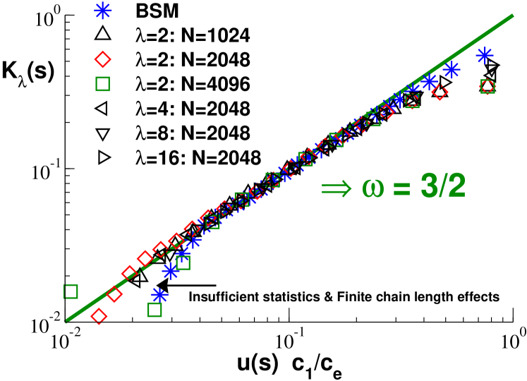
Figure 7: (Color online) Plot of $K_{\lambda}(s)$ as a function of $u(s)c_{1}/c_{\text{e}}\sim 1/\sqrt{s}$ using the measured $u(s)\equiv\sqrt{24/\pi^{3}}s/\rho R_{\text{e}}(s)^{3}$. For $\lambda=2$ (corresponding to two segments being connected) BFM and BSM data are compared. Several $\lambda$ values are given for $N=2048$ BFM chains. For chain segments with $1\ll s\ll N$ all data sets collapse on the bisection line confirming the so-called “recursion relation” $K_{\lambda}\approx u$ proposed by Semenov and Johner Semenov and Johner (2003). The statistics becomes insufficient for large $s$ (left bottom corner). Systematic deviations arise for $s\rightarrow N$ due to additional finite-$N$ effects.

As was emphasized in Sec. II.1 the observed swelling is due to an entropic repulsion between chain segments induced by the incompressibility of the melt. To stress the role of chain connectivity we repeat the general scaling argument given above in a form originally proposed by Semenov and Johner for ultrathin films Semenov and Johner (2003). As shown in Fig. 7 we test the relation

$$K_{\lambda}(s)\equiv\frac{R_{\text{e}}^{2}(\lambda s)-\lambda R_{\text{e}}^{2}(s)}{(\lambda-\sqrt{\lambda})R_{\text{e}}^{2}(s)}\approx u(s)\equiv\frac{s}{\rho R_{\text{e}}(s)^{d}}$$ (21)

with $K_{\lambda}(s)$ being a direct measure of the non-Gaussianity ($\lambda$ being a positive number) comparing the size of a segment of length $\lambda s$ with the size of $\lambda$ segments of length $s$ joined together. (The prefactor $1/(\lambda-\sqrt{\lambda})$ in the definition of $K_{\lambda}(s)$ has been introduced for convenience.) Equivalently, this can be read as a measure for the swelling of a chain where initially the interaction energy $u$ between the segments has been switched off. $K_{\lambda}$ is a functional of $u(s)$ with $K_{\lambda}[u=0]=0$. The analytic expansion of the functional must be dominated by the linear term (as indicated by $\approx$ in the above relation) simply because $u$ is very small. Altogether, Eq. (21) yields a recursion relation relating $R_{\text{e}}(\lambda s)$ with $R_{\text{e}}(s)$ for any $\lambda$ provided $1\ll s<\lambda s\ll N$. It can be solved, leading (in lowest order) to Eq. (5) with $p=1$. This may be seen from the ansatz $R_{\text{e}}^{2}(s)=b_{\text{e}}^{2}s(1-c_{\text{e}}/s^{\omega-1}+\ldots)$ which readily yields $\omega=3/2$ and $c_{\text{e}}\approx 1/\rho b_{\text{e}}^{3}$.

Eq. (21) has been validated directly in Fig. 7 for $\lambda=2$ (corresponding to two segments of length $s$ joined together) for the BFM and the BSM as indicated. In addition, for BFM chains of length $N=2048$ several values of $\lambda$ have been given. As suggested by Eq. (4), we have plotted $K_{\lambda}(s)$ as a function of $(c_{1}/c_{\text{e}})\ u(s)$ with $u(s)\equiv\sqrt{24/\pi^{3}}s/\rho R_{\text{e}}^{3}(s)\approx c_{\text{e}}/\sqrt{s}$. The prefactor of $u(s)$ allows a convenient comparison with Fig. 5. Note the perfect data collapse for all data sets. More importantly, the predicted linearity is well confirmed for large segments ($1\ll s$) and this without any tunable parameter for the vertical axis, as was needed in the previous Figs. 5 and 6.

IV.3 Intrachain bond-bond correlations

Expectation from Flory’s hypothesis.

An even more striking violation of Flory’s ideality hypothesis may be obtained by computing the bond-bond correlation function, defined by the first Legendre polynomial $P(s)=\left<{\bf l}_{m=n+s}\cdot{\bf l}_{n}\right>/l^{2}$ where the average is performed, as before, over all possible pairs of monomers $(n,m=n+s)$ . Here, ${\bf l}_{i}={\bf r}_{i+1}-{\bf r}_{i}$ denotes the bond vector between two adjacent monomers $i$ and $i+1$ and $l^{2}=\left<{\bf l}^{2}_{n}\right>_{n}$ the mean-squared bond length. The bond-bond correlation function is generally believed to decrease exponentially Flory (1988). This belief is based on the few simple single chain models which have been solved rigorously Flory (1988); Kratky and Porod (1949) and on the assumption that all long range interactions are negligible on distances larger than the screening length $\xi$. Hence, only correlations along the backbone of the chains are expected to matter and it is then straightforward to work out that an exponential cut-off is inevitable due to the multiplicative loss of any information transferred recursively along the chain Flory (1988).

Asymptotic behavior in the melt.

That this reasoning must be incorrect follows immediately from the relation

$$P(s)=\frac{1}{2l^{2}}\frac{d^{2}}{ds^{2}}R_{\text{e}}^{2}(s)$$ (22)

expressing the bond-bond correlation function as the curvature of the second moment of the segment size distribution. It is obtained from the identity $\left<{\bf l}_{n}\cdot{\bf l}_{m}\right>=\left<\partial_{n}{\bf r}_{n}\cdot\partial_{m}{\bf r}_{m}\right>=-\partial_{n}\partial_{m}\left<{\bf r}^{2}_{nm}\right>/2$. (Note that the velocity correlation function is similarly related to the second derivative of the mean-square displacement with respect to time Hansen and McDonald (1986).) Hence, $P(s)$ allows us to probe directly the non-Gaussian corrections without any ideal contribution. This relation together with Eq. (5) suggests an algebraical decay $P(s)=c_{\text{P}}/s^{\omega}$ with

$$\omega=3/2\ ,\ c_{\text{P}}=c_{1}\ (b_{\text{e}}/l)^{2}/8\approx\frac{1}{\rho l^{2}b_{\text{e}}}$$ (23)

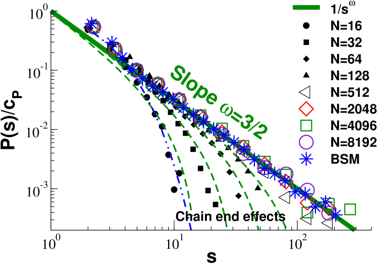
Figure 8: (Color online) The bond-bond correlation function $P(s)/c_{\text{P}}$ as a function of the curvilinear distance $s$. Various chain lengths are given for BFM. Provided that $1\ll s\ll N$, all data sets collapse on the power law slope with exponent $\omega=3/2$ (bold line) as predicted by Eq. (23). The dash-dotted curve $P(s)\approx\exp(-s/1.5)$ shows that exponential behavior is only compatible with very small chain lengths. The dashed lines correspond to the theoretical prediction, Eq. (24), for short chains with $N=16,32,64$ and $128$ (from left to right).

of the bond-bond correlation function for dense solutions and melts, rather than the exponential cut-off expected from Flory’s hypothesis. This prediction (bold line) is perfectly confirmed by the larger chains ($N>256$) indicated in Fig. 8. In principle, the swelling coefficient, $c_{1}\sim c_{\text{P}}$, may also be obtained from the power law amplitude of the bond-bond correlation function, however, to lesser accuracy than by the previous method (Fig. 5). One reason is that $P(s)$ decays very rapidly and does not allow a precise fit beyond $s\approx 10^{2}$. The values of $c_{\text{P}}$ obtained from $c_{1}$ are indicated in Tab. 2. Data from the BSM have also been included in the figure to demonstrate the universality of the result. The vertical axis has been rescaled with $c_{\text{P}}$ which allows to collapse the data of both models.

Finite chain-size corrections.

As can be seen for $N=16$, exponentials are compatible with the data of short chains. This might explain how the power law scaling has been overlooked in previous numerical studies, since good statistics for large chains ($N>1000$) has only become available recently. However, it is clearly shown that $P(s)$ approaches systematically the scale free asymptote with increasing $N$. The departure from this limit is fully accounted for by the theory if chain end effects are carefully considered (dashed lines). Generalizing Eq. (23) and using the Padé approximation, Eq. (17), perturbation theory yields

$$P(s)=\frac{c_{\text{P}}}{s^{3/2}}\frac{1+3x+5x^{2}}{1+x}(1-x)^{2}$$ (24)

where we have set $x=\sqrt{s/N}$. For $x\ll 1$ this is consistent with Eq. (23). In the limit of large $s\rightarrow N$, the correlation functions vanish rigorously as $P(s)\propto(1-x)^{2}$. Considering that non-universal features cannot be neglected for short chain properties and that the theory does not allow for any free fitting parameter, the agreement found in Fig. 8 is rather satisfactory.

IV.4 Higher moments and associated coefficients

Effective bond length and empirical swelling coefficients.

The preceding discussion focused on the second moment of the segmental size distribution $G(r,s)$. We have also computed for both models higher moments $\left<{\bf r}^{2p}\right>$ with $p\leq 5$. If traced in log-linear coordinates as $y=(6^{p}p!\left<{\bf r}^{2p}\right>/(2p+1)!s^{p})^{1/p}$ vs. $x=s$ higher moments approach $b_{\text{e}}^{2}$ from below — just as the second moment presented in Fig. 4. The deviations from ideality are now more pronounced and increase with $p$ (not shown). The moments are compared in Fig. 6 with Eq. (5) where they are rescaled as $y=K_{p}(s)$ as defined in Eq. (1) and plotted as functions of $x=\frac{3(2^{p}p!p)^{2}}{2(2p+1)!}\ \frac{c_{p}}{\sqrt{s}}$. The prediction is indicated by bold lines. It is important that the same effective bond length $b_{\text{e}}$ is obtained from the analysis of all functions $K_{p}(s)$ as illustrated in Fig. 6. Otherwise we would regard equilibration and statistics as insufficient.

The empirical swelling coefficients $c_{p}$ are obtained, as above in Sec. IV.1, by shifting the data horizontally. A good agreement with the expected $c_{p}/c_{\text{e}}\approx 1$ is found for both models and all moments as may be seen from Tab. 2. This confirms the renormalization of the Kuhn segment $b\rightarrow b_{\text{e}}$ of the Gaussian reference chain in agreement with our discussion in Sec. II.2. Otherwise we would have measured empirical coefficients decreasing strongly as $c_{p}/c_{\text{e}}\approx(b/b_{\text{e}})^{2p-3}$ with $p$. Since the effective bond length of non-interacting chains are known for the BFM ($b\approx 2.688$) and the BSM ($b\approx 0.97$), one can simply check, say for $p=5$, that the non-renormalized values would correspond to the ratios $c_{5}/c_{\text{e}}\approx(2.688/3.244)^{7}\approx 0.3$ for the BFM and $c_{5}/c_{\text{e}}\approx(0.97/1.34)^{7}\approx 0.1$ for the BSM. This is clearly not consistent with our data.

It should be emphasized that both coefficients $b_{\text{e}}$ and $c_{p}$ are more difficult to determine for large $p$, since the linear regime for $x\ll 1$ in the representation chosen in Fig. 6 becomes reduced. For large $x\gg 1$ one finds that $y(x)\to 1$, i.e. $\left<{\bf r}^{2p}\right>/b_{\text{e}}^{2p}s^{p}\to 0$. This trivial departure from both Gaussianity and the $1/\sqrt{s}$-deviations we try to describe, is due to the finite extensibility of chain segments of length $s$ which becomes more marked for larger moments probing larger segment sizes. The data collapse for both $x$-regimes is remarkable, however. Incidentally, it should be noted that for the BSM the empirical swelling coefficients are slightly larger than expected. At present we do not have a satisfactory explanation for this altogether minor effect, but it might be attributed to the fact that neighbouring BSM beads along the chain strongly interpenetrate — an effect not considered by the theory.

Non-Gaussian parameter $\alpha_{p}$.

The failure of Flory’s hypothesis can also be demonstrated by means of the standard non-Gaussian parameter

$$\alpha_{p}(s)\equiv 1-\frac{6^{p}p!}{(2p+1)!}\frac{\left<{\bf r}_{nm}^{2p}\right>}{\left<{\bf r}_{nm}^{2}\right>^{p}}$$ (25)

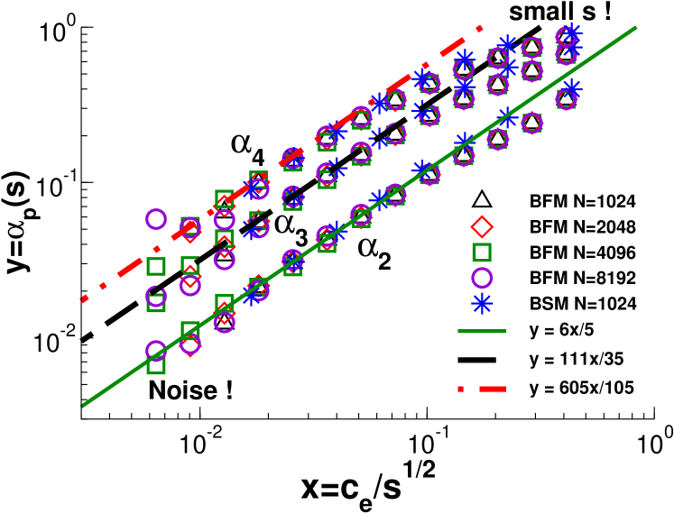
Figure 9: (Color online) Non-Gaussian parameter $\alpha_{p}(s)$ computed for the end-to-end distance of chain segments as a function of $c_{\text{e}}/\sqrt{s}$. Perfect data collapse for all chain lengths and both simulation models is obtained for each $p$. A linear relationship over nearly two orders of magnitude is found as theoretically expected. Data for three moments ($p=2,3,4$) are indicated showing a systematic increase of non-Gaussianity with $p$. The data curvature for small $s$ becomes more pronounced for larger $p$.

comparing the $2p$-th moment with the second moment ($p=1$). In contrast to the closely related parameter $K_{p}(s)$ this has the advantage that here two measured properties are compared without any tuneable parameter, such as $b_{\text{e}}$, which has to be fitted first. Fig. 9 presents $\alpha_{p}(s)$ vs. $c_{\text{e}}/\sqrt{s}$ for the three moments with $p=2,3,4$. For each $p$ we find perfect data collapse for all chain lengths and both models and confirm the linear relationship $\alpha_{p}(s)\approx u(s)$ expected. The lines indicate the theoretical prediction

$$\alpha_{p}(s)=\left(\frac{3\ (2^{p}p!p)^{2}}{2\ (2p+1)!}-p\right)\frac{c_{\text{e}}}{\sqrt{s}}$$ (26)

which can be derived from Eq. (5) by expanding the second moment in the denominator. An alternative derivation based on the coefficients of the expansion of the generating function $G(q,s)$ in $q^{2}$ is indicated by Eq. (35) in the Appendix. Having confirmed above that $c_{p}/c_{\text{e}}\approx 1$, we assume in Eq. (26) that $c_{p}=c_{\text{e}}$ to simplify the notation. The prefactors $6/5$, $111/35$ and $604/105$ for $p=2$, $3$ and $4$ respectively are nicely confirmed. They increase strongly with $p$, i.e. the non-Gaussianity becomes more pronounced for larger moments as already mentioned. Note also the curvature of the data at small $s$ due to the finite extensibility of the segments which becomes more marked for higher moments. If one plots $\alpha_{p}(s)$ as a function of the r.h.s. of Eq. (26) all data points for all moments and even for too small $s$ collapse on one master curve (not shown) — just as we have seen before in Fig. (6).

Correlations of different directions.

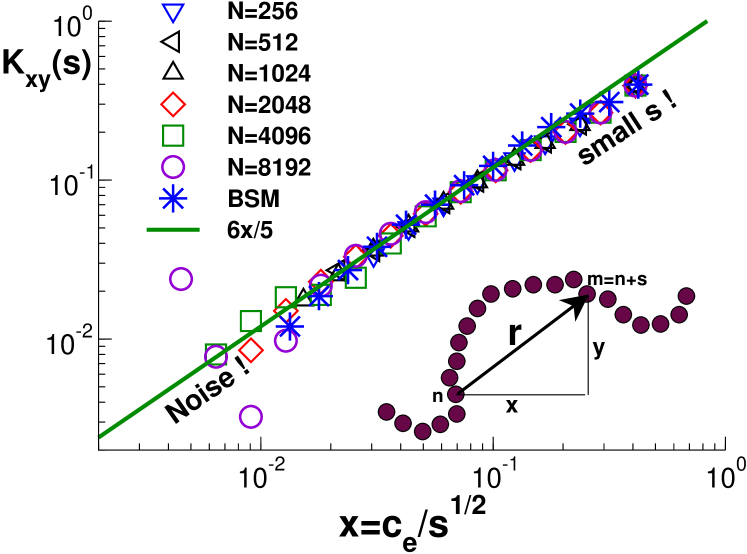
Figure 10: (Color online) Plot of $K_{xy}(s)=1-\left<x^{2}y^{2}\right>/\left<x^{2}\right>\left<y^{2}\right>$ averaged over all pairs of monomers ($n,m=n+s$) and three different direction pairs as a function of $c_{\text{e}}/\sqrt{s}$. As indicated by the sketch at the bottom of the figure, $K_{xy}(s)$ measures the correlation of the components of the segment vector ${\bf r}$. All data points collapse and show again a linear relationship $K_{xy}\approx u(s)$. Different directions are therefore coupled! No curvature is observed over two orders of magnitude confirming that higher order perturbation corrections are negligible. Noise cannot be neglected for large $s>100$ and finite segment-size effects are visible for $s\approx 1$.

A similar correlation function is presented in Fig. 10 which measures the non-Gaussian correlations of different spatial directions. It is defined by

$$K_{xy}(s)\equiv 1-\frac{\left<x^{2}\ y^{2}\right>}{\left<x^{2}\right>\left<y^{2}\right>}$$ (27)

for the two spatial components $x$ and $y$ of the vector ${\bf r}$ as illustrated by the sketch given at the bottom of Fig. 10. Symmetry allows to average over the three pairs of directions $(x,y)$, $(x,z)$ and $(x,z)$. Following the general scaling argument given in Sec. II we expect $K_{xy}(s)\approx u(s)\approx c_{\text{e}}/\sqrt{s}$ which is confirmed by the perturbation result

$$K_{xy}(s)=\frac{6}{5}\frac{c_{\text{e}}}{\sqrt{s}}=K_{2}(s).$$ (28)

This is nicely confirmed by the linear relationship found (bold line) on which all data from both simulation models collapse perfectly. The different directions of chain segments are therefore coupled. As explained in the Appendix (Eq. (36)), $K_{xy}(s)$ and $\alpha_{2}(s)$ must be identical if the Fourier transformed segmental size distribution $G(q,s)$ can be expanded in terms of $q^{2}$ and this irrespective of the values the expansion coefficients take. Fig. 10 confirms, hence, that our computational systems are perfectly isotropic and tests the validity of the general analytical expansion.

The correlation function $K_{xy}$ is of particular interest since the zero-shear viscosity should be proportional to $\left<\sigma_{xy}^{2}\right>\sim\left<x^{2}y^{2}\right>=\left<x^{2}\right>\left<y^{2}\right>(1-K_{xy}(s))$. We assume here following Edwards Doi and Edwards (1986) that only intrachain stresses contribute to the shear stress $\sigma_{xy}$. Hence, our results suggest that the classical calculations Doi and Edwards (1986) — assuming incorrectly $K_{xy}=0$ — should be revisited.

IV.5 The segmental size distribution

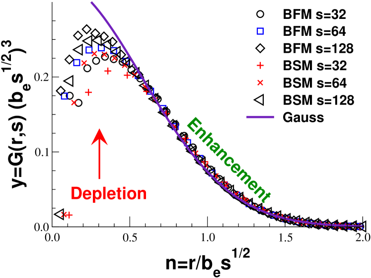
Figure 11: (Color online) Segment size distribution $y=G(r,s)(b_{\text{e}}s^{1/2})^{3}$ vs. $n=r/b_{\text{e}}s^{1/2}$ for several $s$ as indicated in the figure. Only data for BFM with $N=2048$ and BSM with $N=1024$ are presented. (A similar plot can be achieved by renormalizing the axes using $R_{\text{e}}(s)$ instead of $b_{\text{e}}s^{1/2}$). The bold line denotes the Gaussian behaviour $y=(3/2\pi)^{3/2}\exp(-3n^{2}/2)$. One sees that compared to this reference the measured distributions are depleted for small $n\ll 1$ (where the data does not scale) and enhanced for $n\approx 1$.

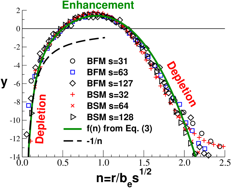
Figure 12: (Color online) Deviation $\delta G(r,s)=G(r,s)-G_{0}(r,s)$ of the measured segmental size distribution from the Gaussian behavior $G_{0}(r,s)$ expected from Flory’s hypothesis for several $s$ and both models as indicated in the figure. As suggested by Eq. (3), we have plotted $y=(\delta G(r,s)/G_{0}(r,s))/(c_{\text{e}}/\sqrt{s})$ as a function of $n=r/b_{\text{e}}\sqrt{s}$. The Gaussian reference distribution has been computed according to Eq. (2) for the measured effective bond length $b_{\text{e}}$. A close to perfect data collapse is found for both models. This shows that the deviation scales linearly with $u(s)\approx c_{\text{e}}/\sqrt{s}$, as expected. The bold line indicates the universal function of $f(n)$ predicted by Eq. (3).

We turn finally to the segmental size distribution $G(r,s)$ itself which is presented in Figs. 11, 12 and 13. From the theoretical point of view $G(r,s)$ is the most fundamental property from which all others can be derived. It is presented last since it is computationally more demanding — at least if high accuracy is needed — and coefficients such as $b_{\text{e}}$ may be best determined directly from the moments. The normalized histograms $G(r,s)$ are computed by counting the number of segment vectors between $r-dr/2$ and $r+dr/2$ with $dr$ being the width of the bin and one divides then by the spherical bin volume. Since the BFM model is a lattice model, this volume is not $4\pi r^{2}dr$ but given by the number of lattice sites the segment vector can actually point to for being allocated to the bin. Incorrect histograms are obtained for small $r$ if this is not taken into account. (Averages are taken over all segments and chains, just as before.) Clearly, non-universal physics must show up for small vector length $r$ and small curvilinear distance $s$ and we concentrate therefore on values $r\gg\sigma$ and $s\geq 31$.

When plotted in linear coordinates as in Fig. 11, $G(r,s)$ compares roughly with the Gaussian prediction $G_{0}(r,s)$ given by Eq. (2), but presents a distinct depletion for small segment sizes with $n\equiv r/b_{\text{e}}\sqrt{s}\ll 1$ and an enhanced regime for $n\approx 1$. A second depletion region for large $n\gg 1$ — expected from the finite extensibility of the segments — can be best seen in the log-log representation of the data (not shown). To analyse the data it is better to consider instead of $G(r,s)$ the relative deviation $\delta G(r,s)/G_{0}(r,s)=G(r,s)/G_{0}(r,s)-1$ which should further be divided by the strength of the segmental correlation hole, $c_{\text{e}}/\sqrt{s}$. As presented in Fig. 12 this yields a direct test of the key relation Eq. (3) announced in the Introduction. The figure demonstrates nicely the scaling of the data for all $s$ and for both models. It shows further a good collapse of the data close to the universal function $f(n)$ predicted by theory (bold line). Note that the depletion scales as $1/n$ for small segment sizes (dashed line). The agreement of simulation and theory is by all standards remarkable. (Obviously, error bars increase strongly for $n\gg 1$ where $G_{0}(r,s)$ decreases strongly. The regime for very large $n$ where the finite extensibility of segments matters has been omitted for clarity.) We emphasize that this scaling plot depends very strongly on the value $b_{\text{e}}$ which is used to calculate the Gaussian reference distribution.

If a precise value is not available we recommend to use instead the scaling variable $m=r/R_{\text{e}}(s)$ for the horizontal axis, i.e. to replace the scale $b_{\text{e}}\sqrt{s}$ estimated from the behaviour of asymptotically long chains by the measured (mean-squared) segment size for the given $s$. The Gaussian reference distribution is then accordingly $G_{0}(m,R_{\text{e}}(s))=(3/2\pi R_{\text{e}}(s)^{2})\exp(-\frac{3}{2}m^{2})$. The corresponding scaling plot is given in Fig. 13. It is similar and of comparable quality as the previous plot. Changing the scaling variable from $n=r/b_{\text{e}}\sqrt{s}$ to $m=r/R_{\text{e}}(s)\approx(r/b_{\text{e}}\sqrt{s})(1+c_{\text{e}}/2\sqrt{s})$ changes somewhat the universal function. Expanding the previous result, Eq. (3), this adds even powers of $m$ to the function $f(n)$ given in Eq. (3)

$$f(n)\Rightarrow f(m)=\sqrt{\frac{3\pi}{32}}\left(-\sqrt{\frac{24}{\pi}}-\frac{2}{m}+9m+\sqrt{\frac{24}{\pi}}m^{2}-\frac{9}{2}m^{3}\right).$$ (29)

That the two additional terms in the function are correct can be seen by computing the second moment $4\pi\int drr^{4}\delta G(r,s)$ which must vanish by construction. The rescaled relative deviation is somewhat broader than in the previous plot due to the additional term scaling as $m^{2}$. As already stressed this scaling does not rely on the effective bond length $b_{\text{e}}$ and is therefore more robust. It has the nice feature that it underlines that there is only one characteristic length scale relevant for the swelling induced by the segmental correlation hole, the typical size of the chain segment itself.

V Conclusion

Issues covered and central theoretical claims.

We have revisited Flory’s famous ideality hypothesis for long polymers in the melt by analyzing both analytically and numerically the segmental size distribution $G(r,s)$ and its moments for chain segments of curvilinear length $s$. We have first identified the general mechanism that gives rise to deviations from ideal chain behavior in dense polymer solutions and melts (Sec. II). This mechanism rests upon the interplay of chain connectivity and the incompressibility of the system which generates an effective repulsion between chain segments (Fig. 2). This repulsion scales like $u(s)\approx c_{\text{e}}/\sqrt{s}$ where the “swelling coefficient” $c_{\text{e}}\approx 1/b_{\text{e}}^{3}\rho$ sets the strength of the interaction. It is strong for small segment length $s$, but becomes weak for $s\rightarrow N$ in the large-$N$ limit. The overall size of a long chain thus remains almost ‘ideal’, whereas subchains are swollen as described by Eq. (5). Most notably, the relative deviation $\delta G(r,s)/G_{0}(r,s)$ of the segmental size distribution from Gaussianity should be proportional to $u(s)$. As a function of segment size $r$, the repulsion manifests itself by a strong $1/r$-depletion at short distances $r\ll b_{\text{e}}\sqrt{s}$ and a subsequent shift of the histogram to larger distances (Eq. (3)).

Summary of computational results.

Using Monte Carlo and molecular dynamics simulation of two coarse-grained polymer models we have verified numerically the theoretical predictions for long and flexible polymers in the bulk. We have explicitly checked (e.g., Figs. 7, 9, 13) that the relative deviations from Flory’s hypothesis scale indeed as $1/\sqrt{s}$. Especially, the measurement of the bond-bond correlation function $P(s)$, being the second derivative of the second moment of $G(r,s)$ with respect of $s$, allows a very precise verification (Fig. 8) and shows that higher order corrections beyond the first-order perturbation approximation must be small. The most central and highly non-trivial numerical verification concerns the data collapse presented in Figs. 12 and 13 for the segmental size distribution of both computational models. All other statements made in this paper can be derived and understood from this key finding. It shows especially that the swelling coefficient $c_{\text{e}}$ must be close to the predicted value, Eq. (4).

It is well known Muthukumar and Edwards (1982) that the effective bond length is difficult to predict at low compressibility and no attempt has been done to do so in this paper. We show instead how the systematic swelling of chain segments – once understood – may be used to extrapolate for the effective bond length of asymptotically long chains. Figs. 5 and 6 indicate how this may be done using Eq. (5). The high precision of our data is demonstrated in Fig. 12 by the successful scaling of the segmental size distribution.

For several moments $\left<{\bf r}^{2p}\right>$ we have also fitted empirical swelling coefficients $c_{p}$ using Eq. (5). In contrast to the effective bond length $b_{\text{e}}$ these coefficients are rather well predicted by one-loop perturbation theory if the bond length $b$ of the reference Hamiltonian is renormalized to the effective bond length $b_{\text{e}}$, as we have conjectured in Sec. II.2. Since the empirical swelling coefficients, $c_{p}\approx c_{\text{e}}(b/b_{\text{e}})^{2p-3}$, would otherwise strongly depend on the moment taken, as shown in Eq. (12), our numerical data (Tab. 2) clearly imply $b/b_{\text{e}}\approx 1$. Minor deviations found for the BSM samples may be attributed to the fact that monomers along the BSM chains do strongly overlap — an effect not taken into account by the theory. To clarify ultimately this issue we are currently performing a numerical study where we systematically vary both the compressibility and the bond length of the BSM.

General background and outlook.

The most striking result presented in this work concerns the power law decay found for the bond-bond correlation function, $P(s)\propto 1/s^{3/2}$ (Fig. 8). This result suggests an analogy with the well-known long-range velocity correlations found in dense fluids by Alder and Wainwright nearly fourty years ago Alder and Wainwright (1970); Hansen and McDonald (1986). In both cases, the ideal uncorrelated object is a random walker which is weakly perturbed (for $d>2$) by the self-interactions generated by global constraints. Although these constraints are different (momentum conservation for the fluid, incompressibility for polymer melts) the weight with which these constraints increase the stiffness of the random walker is always proportional to the return probability. It can be shown that the correspondence of both problems is mathematically rigorous if the fluid dynamics is described on the level of the linearized Navier-Stokes equations Beckrich et al. (2007b).

We point out that the physical mechanism which has been sketched above is rather general and should not be altered by details such as a finite persistence length — at least not as long as nematic ordering remains negligible and the polymer chains are sufficiently long. (Similarly, velocity correlations in dense liquids must show an analytical decay for sufficiently large times irrespective of the particle mass and the local static structure of the solution.) While this paper focused exclusively on scales beyond the correlation length of the density fluctuations, i.e. $q\xi\ll 1$ or $s/g\gg 1$, where the polymer solution appears incompressible, effects of finite density and compressibility can be readily described within the same theoretical framework and will be presented elsewhere Beckrich et al. (2007b). To test our predictions, flexible chains should be studied preferentially, since the chain length required for a clear-cut description increases strongly with persistence length. This is in fact confirmed by preliminary and on-going simulations using the BSM algorithm.

In this work we have only discussed properties in real space as a function of the curvilinear distance $s$. These quantities are straightforward to compute in a computer simulation but are barely experimentally relevant. The non-Gaussian deviations induced by the segmental correlation hole arise, however, also for an experimentally accessible property, the intramolecular form factor (single chain scattering function) $F(q)$. As explained at the end of the Appendix, the form factor can be readily obtained by integrating the Fourier transformed segmental size distribution given in Eq. (3). This yields

$$q^{2}F(q)\approx\frac{12}{b_{\text{e}}^{2}}\left(1-\frac{3}{8}\frac{b_{\text{e}}q}{b_{\text{e}}^{3}\rho}\right)$$ (30)

in agreement with the result obtained in Refs. Beckrich et al. (2007a); Wittmer et al. (2007a) by direct calculation of the form factor for very long equilibrium polymers. As a consequence of this, the Kratky plot ($q^{2}F(q)$ vs. wave vector $q$) should not exhibit the plateau expected for Gaussian chains in the scale-free regime, but rather noticeable non-monotonic deviations. See Fig. 3 of Wittmer et al. (2007a). This result suggests to revisit experimentally this old pivotal problem of polymer science.

Our work is part of a broader attempt to describe systematically the effects of correlated density fluctuations in dense polymer systems, both for static Semenov (1996); Semenov and Johner (2003); Semenov and Obukhov (2005); Obukhov and Semenov (2005) and dynamical Semenov (1997); Semenov and Rubinstein (1998); Mattioni et al. (2003) properties. An important unresolved question is for instance whether the predicted long-range repulsive forces of van der Waals type (“Anti-Casimir effect”) Semenov and Obukhov (2005); Obukhov and Semenov (2005) are observable, for instance in the oscillatory decay of the standard density pair-correlation function of dense polymer solutions. Since the results presented here challenge an important concept of polymer physics, they should hopefully be useful for a broad range of theoretical approaches which commonly assume the validity of the Gaussian chain model down to molecular scales Curro et al. (1991); Fuchs (1997); Schulz et al. (2004). This study shows that a polymer in dense solutions should not be viewed as one soft sphere (or ellipsoid) Likos (2001); Eurich and Maass (2001); Yatsenko et al. (2004), but as a hierarchy of nested segmental correlation holes of all sizes aligned and correlated along the chain backbone (Fig. 2 (b)). We note that similar deviations from Flory’s hypothesis have been reported recently for linear polymers Curro et al. (1991); Schäfer et al. (2000); Auhl et al. (2003) and polymer gels and networks Sommer and Saalwächter (2005); Svaneborg et al. (2005). The repulsive interactions should also influence the polymer dynamics, since strong deviations from Gaussianity are expected on the scale where entanglements become important, hence, quantitative predictions for the entanglement length $N_{\text{e}}$ have to be regarded with more care. The demonstrated swelling of chains should be included in the popular primitive path analysis for obtaining $N_{\text{e}}$ Everaers et al. (2004), especially if ‘short’ chains ($N<500$) are considered. The effect could be responsible for observed deviations from Rouse behavior Paul et al. (1991); Paul and Smith (2004) as may be seen by considering the correlation function $C_{pq}\equiv\left<{\bf X}_{p}\cdot{\bf X}_{q}\right>$ of the Rouse modes ${\bf X}_{p}=\frac{1}{N}\int_{n=0}^{N}dn{\bf r}_{n}\cos(np\pi/N)$ where $p,q=0,\ldots,N-1$ Verdier (1966); Doi and Edwards (1986). Using $({\bf r}_{n}-{\bf r}_{m})^{2}={\bf r}_{n}^{2}+{\bf r}_{m}^{2}-2{\bf r}_{n}\cdot{\bf r}_{m}$ for the segment size, this correlation function can be readily expressed as an integral over the second moment of the segmental size distribution

$$C_{pq}=-\frac{1}{2N^{2}}\int_{0}^{N}dn\int_{0}^{N}dm\left<({\bf r}_{n}-{\bf r}_{m})^{2}\right>\cos(np\pi/N)\cos(mp\pi/N)$$ (31)

which can be solved using our result Eq. (5). This implies for instance for $p=q$ that

$$C_{pp}=\frac{Nb_{\text{e}}^{2}}{2(\pi p)^{2}}\left(1-\frac{\pi}{\sqrt{8}}\frac{c_{1}}{\sqrt{N/p}}\right).$$ (32)

The bracket entails an important correction with respect to the classical description given by the prefactor Doi and Edwards (1986). We are currently working out how static corrections, such as those for $C_{pp}$, may influence the dynamics for polymer chains without topological constraints. (This may be realized, e.g., within the BFM algorithm by using the L26 moves described in Sec. III.1.)

Moreover, for thin polymer films of width $H$ the repulsive interactions are known to be stronger than in the bulk Semenov and Johner (2003). This provides a mechanism to rationalize the trend towards swelling observed experimentally Jones et al. (1999) and confirmed computationally Cavallo et al. (2005):

$$1-\frac{R_{x}^{2}(s)}{b_{x}^{2}s}=\log(s)/H.$$ (33)

(Prefactors omitted for clarity.) Here $R_{x}(s)$ and $b_{x}$ denote the components of the segment size and the effective bond length parallel to the film. It also explains the (at first sight surprising) systematic increase of the polymer dynamics with decreasing film thickness Meyer et al. (2007). Specifically, the parallel component of the monomer mean-squared displacement $g_{x}(t)$ is expected to scale as $g_{x}(t)\approx R_{x}^{2}(s(t))\propto t^{1/4}(1+\log(t)/H)$ for long reptating chains where $s(t)\propto t^{1/4}$ Doi and Edwards (1986). (The corresponding effect for the three-dimensional bulk should be small, however.) For the same reason (flexible) polymer chains close to container walls must be more swollen and, hence, faster on intermediate time scales than their peers in the bulk.

Appendix A Moments of the segmental size distribution and their generating function

Higher moments of the segmental size distribution $G(r,s)$ can be systematically obtained from its Fourier transformation

$$G(q,s)=\int d^{3}{\bf r}\ G(r,s)\ \exp(i{\bf q\cdot r}),$$

which is in this context sometimes called the “generating function” van Kampen (1992). For an ideal Gaussian chain, the generating function is then $G_{0}(q,s)=\exp(-sq^{2}a^{2})$ where we have used $a^{2}=b^{2}/6$ instead of the bond length $b^{2}$ to simplify the notation. Moments of the size distribution are given by proper derivatives of $G(q,s)$ taken at $q=0$. For example, $\langle{\bf r}^{2p}\rangle=(-1)^{p}\Delta^{p}G(q,s)_{q=0}$ (with $\Delta$ being the Laplace operator with respect to the wave vector ${\bf q}$). A moment of order $2p$ is, hence, linked to only one coefficient $A_{2p}$ in the systematic expansion, $G(q,s)=\sum_{p=0}A_{2p}q^{2p}$, of $G(q,s)$ around $q=0$. For our example this implies

$$\left<{\bf r}^{2p}\right>=(-1)^{p}(2p+1)!\ A_{2p}$$ (34)

in general and more specifically for a Gaussian distribution ${\langle{\bf r}^{2p}\rangle}_{0}=\frac{(2p+1)!}{p!}s^{p}a^{2p}$. The non-Gaussian parameters read, hence,

$$\alpha_{p}(s)\equiv 1-\frac{6^{p}p!}{(2p+1)!}\frac{\langle{\bf r}^{2p}\rangle}{\langle{\bf r}^{2}\rangle^{p}}=1-p!\ \frac{A_{2p}}{A_{2}^{p}},$$ (35)

which implies (by construction) $\alpha_{p}=0$ for a Gaussian distribution. As various moments of the same global order $2p$ are linked to the same $A_{2p}$ they differ by a multiplicative constant independent of the details of the (isotropic) distribution $G(q,s)$. For example, $\langle{\bf r}^{2}\rangle=6|A_{2}|$, $\langle{\bf r}^{4}\rangle=120A_{4}$, $\langle x^{2}\rangle=\langle y^{2}\rangle=2|A_{2}|$, $\langle x^{2}y^{2}\rangle=8A_{4}$ with $x$ and $y$ denoting the spatial components of the segment vector ${\bf r}$. Using Eq. (35) for $p=2$ it follows that

$$K_{xy}(s)\equiv 1-\frac{\langle x^{2}y^{2}\rangle}{\langle x^{2}\rangle\langle y^{2}\rangle}=1-2\frac{A_{4}}{A_{2}^{2}}=\alpha_{2}(s),$$ (36)

i.e. the properties $\alpha_{2}(s)$ and $K_{xy}(s)$ discussed in Figs. 9 and 10 must be identical in general provided that $G(q,s)$ is isotropic and can be expanded in $q^{2}$.

We turn now to specific properties of $G(q,s)$ computed for formally infinite polymer chains in the melt. In practice, these results are also relevant for small segments in large chains, $N\gg s\gg 1$, and, especially, for segments located far from the chain ends. These chains are nearly Gaussian and the generating function can be written as $G(q,s)=G_{0}(q,s)+\delta G(q,s)$ where $\delta G(q,s)=-\langle UG\rangle_{0}+\langle U\rangle_{0}\langle G\rangle_{0}$ is a small perturbation under the effective interaction potential $\tilde{v}(q)$ given by Eq. (9). To compute the different integrals it is more convenient to work in Fourier-Laplace space ($q,t$) with $t$ being the Laplace variable conjugate to $s$:

$$\delta G(q,t)=\int_{0}^{\infty}ds\ \delta G(q,s)e^{-st}.$$

As illustrated in Fig. 14, there a three contributions to this perturbation: one due to interactions between two monomers inside the segment (left panel), one due to interactions between an internal monomer and an external one (middle panel) and one due to interactions between two external monomers located on opposite sides (right panel). In analogy to the derivation of the form factor described in Ref. Beckrich et al. (2007a) this yields:

$$\delta G(q,t) = -\frac{1}{(q^{2}a^{2}+t)^{2}}\frac{v}{4\pi a^{3}}\left(\sqrt{q^{2}a^{2}+t}-\sqrt{t}\right)$$ (37)

$$+ \frac{1}{(q^{2}a^{2}+t)^{2}}\frac{v}{4\pi qa^{2}\xi^{2}}\left(\mbox{Arctan}\left[\frac{qa}{a/\xi+\sqrt{t}}\right]-\frac{qa}{a/\xi+\sqrt{q^{2}a^{2}+t}}\right)$$

$$- \frac{1}{q^{2}a^{2}+t}\frac{2v}{4\pi qa^{4}}\left(\mbox{Arctan}\left[\frac{qa}{a/\xi+\sqrt{t}}\right]-\frac{qa}{a/\xi+\sqrt{q^{2}a^{2}+t}}\right)$$

$$- \frac{v\xi^{2}}{4\pi qa^{6}}\left(\mbox{Arctan}\left[\frac{qa}{\sqrt{t}}\right]-\frac{qa}{\sqrt{q^{2}a^{2}+t}}\right).$$

The graph given in the left panel of Fig. 14 corresponds to the first two lines, the middle panel to the third line and the right panel to the last one. Seeking for the moments we expand $\delta G(q,t)$ around $q=0$. Having in mind chain strands counting many monomers ($s\gg 1$), we need only to retain the most singular terms for $t\rightarrow 0$. Defining the two dimensionless constants $d=v\xi/3\pi a^{4}=12v\xi/\pi b^{4}$ and $c=(3\pi^{3/2}a^{3}\rho)^{-1}=\sqrt{24/\pi^{3}}/b^{3}\rho$ this expansion can be written as

$$\delta G(q,t)= - \frac{1}{1!}\frac{\Gamma(2)}{t^{2}}\ d\ a^{2}q^{2}+\frac{1}{1!}\frac{\Gamma(3/2)}{t^{3/2}}\ c\ a^{2}q^{2}+\ldots$$

$$+ \frac{2}{2!}\frac{\Gamma(3)}{t^{3}}\ d\ a^{4}q^{4}-\frac{1}{2!}\frac{16}{5}\frac{\Gamma(5/2)}{t^{5/2}}\ c\ a^{4}q^{4}+\ldots$$

$$- \frac{3}{3!}\frac{\Gamma(4)}{t^{4}}\ d\ a^{6}q^{6}+\frac{1}{3!}\frac{216}{35}\frac{\Gamma(7/2)}{t^{7/2}}\ c\ a^{6}q^{6}+\ldots$$

$$+ \ldots$$

where we have used Euler’s Gamma function $\Gamma(\alpha)$ Abramowitz and Stegun (1964). The first leading term at each order in $q^{2}$ — being proportional to the coefficient $d$ — ensures the renormalization of the effective bond length. The next term scaling with the coefficient $c$ corresponds to the leading finite strand size correction. Performing the inverse Laplace transformation $\Gamma(\alpha)/t^{\alpha}\rightarrow s^{\alpha-1}$ and adding the Gaussian reference distribution $G_{0}(q,s)$ this yields the $A_{2p}$-coefficients for the expansion of $G(q,s)$ around $q=0$:

$$A_{0} = 1$$

$$A_{2} = -a^{2}s\left(1+d-\frac{c}{\sqrt{s}}\right)$$

$$A_{4} = \frac{1}{2}a^{4}s^{2}\left(1+2d-\frac{16}{5}\frac{c}{\sqrt{s}}\right)$$

$$A_{6} = -\frac{1}{6}a^{6}s^{3}\left(1+3d-\frac{216}{35}\frac{c}{\sqrt{s}}\right)$$

$$A_{8} = \ldots$$ (39)

More generally, one finds

$$A_{2p}=\frac{(-1)^{p}}{p!}(sa^{2})^{p}\left(1+pd-\frac{3(2^{p}p!p)^{2}}{2(2p+1)!}\frac{c}{\sqrt{s}}\right)$$ (40)

From this result and using Eq. (34) one immediately verifies that the moments of the distribution are given by the Eqs. (11) and (12). Using Eq. (35) one justifies similarly Eq. (26) for the non-Gaussian parameter $\alpha_{p}$.

These moments completely determine the segmental distribution $G(r,s)$ which is indicated in Eq. (13). While at least in principle this may be done directly by inverse Fourier-Laplace transformation of the correction $\delta G(q,t)$ to the generating function it is helpful to simplify further Eq. (37). We observe first that $\delta G(q,t)$ does diverge for strictly incompressible systems ($v\rightarrow\infty$) and one must keep $v$ finite in the effective potential whenever necessary to ensure convergence (actually everywhere but in the diagram corresponding to the interaction between two external monomers). Since we are not interested in the wave vectors larger than $1/\xi$ we expand $\delta G(q,t)$ for $\xi\rightarrow 0$ which leads to the much simpler expression

$$\delta G(q,t)\approx-\frac{v\xi q^{2}}{3\pi a^{2}(a^{2}q^{2}+t)^{2}}+\frac{v\xi^{2}}{4\pi a^{6}}\frac{a\sqrt{t}(3a^{2}q^{2}+t)}{(a^{2}q^{2}+t)^{2}}-\frac{v\xi^{2}}{4\pi a^{6}}\frac{\mbox{Arctan}[\frac{aq}{\sqrt{t}}]}{q}+o(v\xi^{3}).$$ (41)

The first term diverges as $\sqrt{v}$ for diverging $v$. It renormalizes the effective bond length in the zero order term which is indicated in the first line of Eq. (13). The next two terms scale both as $v^{0}$. Subsequent terms must all vanish for diverging $v$ and can be discarded. It is then easy to perform an inverse Fourier-Laplace transformation of the two relevant $v^{0}$ terms. This yields

$$\delta G(x,s)=G_{0}(x,s)\frac{c}{\sqrt{s}}\frac{3\sqrt{\pi}}{4}\left(-\frac{2}{x}+\frac{3x}{2}-\frac{x^{3}}{8}\right)$$ (42)

with $x=r/a\sqrt{s}=\sqrt{6}n$. This is consistent with the expression given in the second line of Eq. (13).

We note finally that the intramolecular form factor $F(q)=\frac{1}{N}\sum_{n,m=1}^{N}\left<\exp(i{\bf q}\cdot({\bf r}_{n}-{\bf r}_{m})\right>$ of asymptotically long chains can be readily obtained from Eq. (41). Observing that $\left<\exp(i{\bf q}\cdot({\bf r}_{n}-{\bf r}_{m})\right>=\int d^{3}{\bf r}\exp(i{\bf q}\cdot{\bf r})G(r,s)=G(q,s)$ one finds

$$\delta F(q)=2\int ds\ \delta G(q,s)=2\ \delta G(q,t=0)=-2\frac{v\xi^{2}}{4\pi a^{6}}\frac{\pi/2}{q},$$ (43)

where we used the third term of Eq. (41) in the last step. The first term in Eq. (41) is discarded as before, since it renormalizes the effective bond length in the reference form factor: $F_{0}(q)=12/b^{2}q^{2}\Rightarrow 12/b_{\text{e}}^{2}q^{2}$. It follows, hence, that within first-order perturbation theory

$$F(q)=F_{0}(q)+\delta F(q)\approx F_{0}(q)\left(1-\frac{3}{8}\frac{b_{\text{e}}q}{b_{\text{e}}^{3}\rho}\right)$$ (44)

as indicated by Eq. (30) in the Conclusion. This is equivalent to the result $1/F(q)-1/F_{0}(q)\approx q^{3}/32\rho$ discussed in Refs. Wittmer et al. (2007a); Beckrich et al. (2007a) for polymer melts and anticipated by Schäfer Schäfer (1999) by renormalization group calculations of semidilute solutions.

$N$	$n_{\text{ch}}$	$\tau_{\text{e}}$	$R_{\text{e}}$	$R_{\text{g}}$	$b_{\text{e}}(N)$	$\sqrt{6}b_{\text{g}}(N)$
16	$2^{16}$	$1214$	11.7	4.8	2.998	2.939
32	$2^{15}$	$3485$	17.1	7.0	3.066	3.030
64	$2^{14}$	$1.1\cdot 10^{4}$	24.8	10.1	3.116	3.094
128	8192	$3.3\cdot 10^{4}$	35.6	14.5	3.153	3.139
256	4096	$1.0\cdot 10^{5}$	50.8	20.7	3.179	3.171
512	2048	$3.2\cdot 10^{5}$	72.2	29.5	3.200	3.193
1024	1024	$1.0\cdot 10^{6}$	103	42.0	3.216	3.212
2048	512	$3.2\cdot 10^{6}$	146	59.5	3.227	3.223
4096	256	$9.7\cdot 10^{6}$	207	85.0	3.235	3.253
8192	128	$2.9\cdot 10^{7}$	294	120	3.249	3.248

Table 1: Various static properties of dense BFM melts of number density $\rho=0.5/8$: the chain length $N$, the number of chains $n_{\text{ch}}$ per box, the relaxation time $\tau_{\text{e}}$ characterized by the diffusion of the monomers over the end-to-end distance and corresponding to the circles indicated in Fig. 3, the root-mean-squared chain end-to-end distance $R_{\text{e}}$ and the radius of gyration $R_{\text{g}}$ of the total chain ($s=N-1$). The last two columns give estimates for the effective bond length from the end-to-end distance, $b_{\text{e}}(N)\equiv R_{\text{e}}/(N-1)^{1/2}$, and the radius of gyration, $b_{\text{g}}(N)\equiv R_{\text{g}}/\sqrt{N}$. The dashed line in Fig. 4 indicates $b_{\text{e}}(N)^{2}$. Apparently, both estimates increase monotonicly with $N$ reaching $b_{\text{e}}(N)\approx\sqrt{6}b_{\text{g}}(N)\approx 3.2$ for the largest chains available. Note that $\sqrt{6}b_{\text{g}}(N)<b_{\text{e}}(N)$ for smaller $N$.

Property	BFM	BSM
Length unit	lattice constant	bead diameter
Temperature $k_{\text{B}}T$	1	1
Number density $\rho$	0.5/8	0.84
Linear box size $L$	256	$\leq 62$
Number of monomers $n_{\text{mon}}$	1048576	$\leq 196608$
Largest chain length $N$	8192	1024
Mean bond length $\langle|{\bf l}_{n}|\rangle$	2.604	0.97
$l=\langle{\bf l}_{n}^{2}\rangle^{1/2}$	2.636	0.97
Effective bond length $b_{\text{e}}$	3.244	1.34
$\rho b_{\text{e}}^{3}$	2.13	2.02
$C_{\infty}=(b_{\text{e}}/l)^{2}$	1.52	1.91
$l_{\text{p}}=l(C_{\infty}+1)/2$	3.32	1.41
$c_{\text{e}}\equiv\sqrt{24/\pi^{3}}/\rho b_{\text{e}}^{3}$	0.41	0.44
$c_{1}/c_{\text{e}}$	$1.0$	$1.2$
$c_{2}/c_{\text{e}}$	$1.0$	$1.1$
$c_{3}/c_{\text{e}}$	$1.0$	$1.0$
$c_{4}/c_{\text{e}}$	$1.1$	$1.2$
$c_{5}/c_{\text{e}}$	$1.1$	$0.9$
$c_{\text{P}}=c_{1}(b_{\text{e}}/l)^{2}/8$	0.078	0.124
Dimensionless compressibility $g$	0.245	0.08
Compression modulus $v\equiv 1/g\rho$	66.7	14.9
$G_{\text{z}}\equiv\sqrt{v\rho}/b_{\text{e}}^{3}\rho$	0.96	1.8

Table 2: Comparison of some static properties of dense BFM and BSM melts. The first six rows indicate conventions and operational parameters. The effective bond length $b_{\text{e}}$ and the swelling coefficients $c_{p}$ (defined in Eq. (5)) are determined from the first five even moments of the segmental size distribution. The dimensionless compressibility $g=S(q\rightarrow 0)/\rho$ has been obtained from the total static structure factor $S(q)=\frac{1}{L^{3}}\sum_{k,l=1}^{n_{\text{mon}}}\left<\exp(i{\bf q}\cdot({\bf r}_{k}-{\bf r}_{l}))\right>$ in the zero wave vector limit as shown at the end of Ref. Beckrich et al. (2007a). The values indicated correspond to the asymptotic long chain behavior. Properties of very small chains deviate slightly.

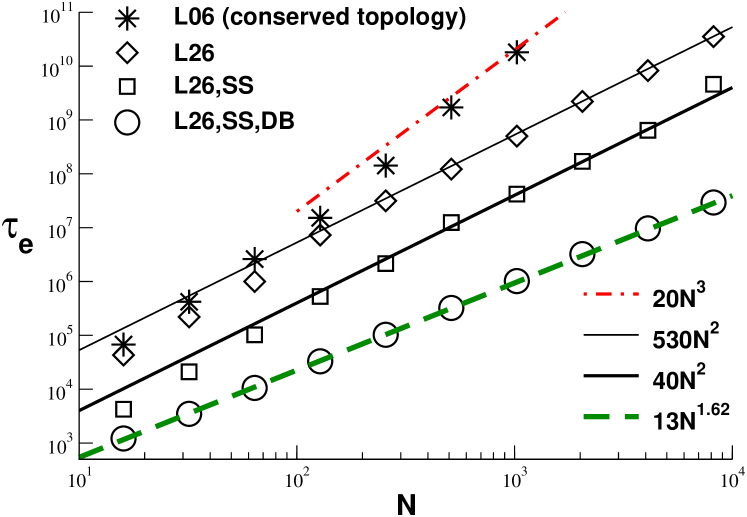
Figure 3: (Color online) Diffusion time $\tau_{\text{e}}$ over the (root-mean-squared) chain end-to-end distance $R_{\text{e}}(N-1)$ as a function of chain length $N$ for different versions of the Bond Fluctuation Model (BFM). All data indicated are for the high number density ($\rho=0.5/8$) corresponding to a polymer melt with half the lattice sites being occupied. We have obtained $\tau_{\text{e}}=R_{\text{e}}^{2}(N-1)/6D_{\text{s}}$ from the self-diffusion coefficient $D_{\text{s}}$ measured from the free diffusion limit of the mean-squared displacement of all monomers $\left<\delta r(t)^{2}\right>=6D_{\text{s}}t$. Data from the classical BFM with topology conserving local Monte Carlo (MC) moves in 6 spatial directions (L06) Paul et al. (1991) are represented as stars. All other data sets use topology violating local MC moves in 26 lattice directions (L26). If only local moves are used, L26-dynamics is even at relatively short times perfectly Rouse like which allows the accurate determination of $D_{\text{s}}$ although the monomers possibly have not yet moved over $R_{\text{e}}(N-1)$ for the largest chain lengths considered. Additional slithering snake (SS) moves increase the efficiency of the algorithm by approximately an order of magnitude (squares,bold line). The power law exponent is changed from $2$ to an empirical $1.62$ (dashed line) if in addition we perform double-bridging (DB) moves.

Figure 14: Interaction diagrams used in reciprocal space for the calculation of $\delta G(q,t)$ in the scale free limit. There exist three nonzero contributions to first-order perturbation, the first involving two points inside the segment (first two lines of Eq. (37)), the second one point inside and one outside the segment (third line of Eq. (37)) and the third one point on either side of the segment (last line of Eq. (37)). Momentum $q$ flows from one correlated point to the other. Integrals are performed over the momentum $k$. Dotted lines denote the effective interactions $\tilde{v}(k)$ given by Eq. (9), bold lines the propagators which carry each a momentum $q$ or $q-k$ as indicated.

References

- Rubinstein and Colby (2003) M. Rubinstein and R. Colby, Polymer Physics (Oxford University Press, 2003).
- Flory (1945) P. J. Flory, J. Chem. Phys. 13, 453 (1945).
- Flory (1949) P. J. Flory, J. Chem. Phys. 17, 303 (1949).
- Flory (1988) P. J. Flory, Statistical Mechanics of Chain Molecules (Oxford University Press, New York, 1988).
- de Gennes (1979) P. G. de Gennes, Scaling Concepts in Polymer Physics (Cornell University Press, Ithaca, New York, 1979).
- Doi and Edwards (1986) M. Doi and S. F. Edwards, The Theory of Polymer Dynamics (Clarendon Press, 1986).
- Edwards (1965) S. Edwards, Proc. Phys. Soc. 85, 613 (1965).
- Edwards (1966) S. Edwards, Proc. Phys. Soc. 88, 265 (1966).
- Edwards (1975) S. Edwards, J.Phys.A: Math.Gen. 8, 1670 (1975).
- Muthukumar and Edwards (1982) M. Muthukumar and S. Edwards, J. Chem. Phys. 76, 2720 (1982).
- Schäfer (1999) L. Schäfer, Excluded Volume Effects in Polymer Solutions (Springer-Verlag, New York, 1999).
- Semenov and Johner (2003) A. N. Semenov and A. Johner, Eur. Phys. J. E 12, 469 (2003).
- Semenov and Obukhov (2005) A. N. Semenov and S. P. Obukhov, J. Phys.: Condens. Matter 17, 1747 (2005).
- Beckrich et al. (2007a) P. Beckrich, A. Johner, A. N. Semenov, S. P. Obukhov, H. C. Benoît, and J. P. Wittmer, Macromolecules (2007a), in press, cond-mat/0701261.
- Beckrich (2006) P. Beckrich, Ph.D. thesis, Université Louis Pasteur, Strasbourg, France (2006).
- Schäfer et al. (2000) L. Schäfer, M. Müller, and K. Binder, Macromolecules 33, 4568 (2000).
- Auhl et al. (2003) R. Auhl, R. Everaers, G. Grest, K. Kremer, and S. Plimpton, J. Chem. Phys. 119, 12718 (2003).
- Wittmer et al. (2004) J. P. Wittmer, H. Meyer, J. Baschnagel, A. Johner, S. P. Obukhov, L. Mattioni, M. Müller, and A. N. Semenov, Phys. Rev. Lett. 93, 147801 (2004), cond-mat/0404457.
- Wittmer et al. (2007a) J. P. Wittmer, P. Beckrich, A. Johner, A. N. Semenov, S. P. Obukhov, H. Meyer, and J. Baschnagel, Europhys. Lett. 77, 56003 (2007a), cond-mat/0611322.
- Wittmer et al. (2007b) J. P. Wittmer, P. Beckrich, F. Crevel, C. C. Huang, A. Cavallo, T. Kreer, and H. Meyer, Computer Physics Communications (2007b), in press, cond-mat/0610359.
- Cavallo et al. (2005) A. Cavallo, M. Müller, J. P. Wittmer, and A. Johner, J. Phys.: Condens. Matter 17, 1697 (2005), cond-mat/0412373.
- Meyer et al. (2007) H. Meyer, T. Kreer, A. Cavallo, J. P. Wittmer, and J. Baschnagel, Eur. Phys. J. Special Topics 141, 167 (2007), cond-mat/0609127.
- Baschnagel et al. (2004) J. Baschnagel, J. P. Wittmer, and H. Meyer, in Computational Soft Matter: From Synthetic Polymers to Proteins, edited by N. Attig (NIC Series, Jülich, 2004), vol. 23, pp. 83–140, cond-mat/0407717.
- Carmesin and Kremer (1988) I. Carmesin and K. Kremer, Macromolecules 21, 2819 (1988).
- Deutsch and Binder (1991) H. Deutsch and K. Binder, J. Chem. Phys 94, 2294 (1991).
- Paul et al. (1991) W. Paul, K. Binder, D. Heermann, and K. Kremer, J. Phys. II 1, 37 (1991).
- Kron (1965) A. Kron, Polym. Sci. USSR 7, 1361 (1965).
- Wall and Mandel (1975) F. Wall and F. Mandel, J. Chem. Phys. 63, 4592 (1975).
- Mattioni et al. (2003) L. Mattioni, J. P. Wittmer, J. Baschnagel, J.-L. Barrat, and E. Luijten, Eur. Phys. J. E 10, 369 (2003), cond-mat/0212433.
- Karayiannis et al. (2002) N. Karayiannis, A. Giannousaki, V. Mavrantzas, and D. Theodorou, J. Chem. Phys. 117, 5465 (2002).
- Banaszak and de Pablo (2003) B. J. Banaszak and J. J. de Pablo, J. Chem. Phys. 119, 2456 (2003).
- Müller et al. (2000) M. Müller, J. P. Wittmer, and J.-L. Barrat, Europhys. Lett. 52, 406 (2000), cond-mat/0006464.
- Kreer et al. (2001) T. Kreer, J. Baschnagel, M. Müller, and K. Binder, Macromolecules 34, 1105 (2001).
- Deutsch (1985) J. M. Deutsch, Phys. Rev. Lett. 54, 56 (1985).
- Semenov (1997) A. N. Semenov, in Theoretical Challenges in the Dynamics of Complex Fluids, edited by T. McLeish (Kluwer, Dordrecht, 1997), pp. 63–86.
- Meyer and Müller-Plathe (2001) H. Meyer and F. Müller-Plathe, J. Chem. Phys. 115, 7807 (2001).
- Meyer and Müller-Plathe (2002) H. Meyer and F. Müller-Plathe, Macromolecules 35, 1241 (2002).
- Kremer and Grest (1990) K. Kremer and G. Grest, J. Chem. Phys. 92, 5057 (1990).
- Allen and Tildesley (1994) M. Allen and D. Tildesley, Computer Simulation of Liquids (Oxford University Press, Oxford, 1994).
- Kratky and Porod (1949) O. Kratky and G. Porod, Rec. Trav. Chim. 68, 1106 (1949).
- Hansen and McDonald (1986) J. Hansen and I. McDonald, Theory of simple liquids (Academic Press, New York, 1986).
- Alder and Wainwright (1970) B. Alder and T. Wainwright, Phys. Rev. A 1, 18 (1970).
- Beckrich et al. (2007b) P. Beckrich, J. P. Wittmer, H. Meyer, S. P. Obukhov, A. N. Semenov, and A. Johner (2007b), in preparation.
- Semenov (1996) A. N. Semenov, Journal de Physique II France 6, 1759 (1996).
- Obukhov and Semenov (2005) S. P. Obukhov and A. N. Semenov, Phys. Rev. Lett. 95, 038305 (2005).
- Semenov and Rubinstein (1998) A. N. Semenov and M. Rubinstein, Eur. Phys. J. B 1, 87 (1998).
- Curro et al. (1991) J. Curro, K. S. Schweizer, G. S. Grest, and K. Kremer, J. Chem. Phys. 91, 1359 (1991).
- Fuchs (1997) M. Fuchs, Z. Phys. B 5, 521 (1997).
- Schulz et al. (2004) M. Schulz, H. Frisch, and P. Reineker, New Journal of Physics 6, 77/1 (2004).
- Likos (2001) C. Likos, Physics Reports 348, 267 (2001).
- Eurich and Maass (2001) F. Eurich and P. Maass, J. Chem. Phys. 114, 7655 (2001).
- Yatsenko et al. (2004) G. Yatsenko, E. J. Sambriski, M. A. Nemirovskaya, and M. Guenza, Phys. Rev. Lett. 93, 257803 (2004).
- Sommer and Saalwächter (2005) J.-U. Sommer and K. Saalwächter, Eur. Phys. J. E 18, 167 (2005).
- Svaneborg et al. (2005) C. Svaneborg, G. Grest, and R. Everaers, Europhys. Lett. 72, 760 (2005).
- Everaers et al. (2004) R. Everaers, S. Sukumaran, G. Grest, C. Svaneborg, A. Sivasubramanian, and K. Kremer, Science 303, 823 (2004).
- Paul and Smith (2004) W. Paul and G. Smith, Rep. Progr. Phys. 67, 1117 (2004).
- Verdier (1966) P. Verdier, J. Chem. Phys. 45, 2118 (1966).
- Jones et al. (1999) R. Jones, S. Kumar, D. Ho, R. Briber, and T. Russell, Nature 400, 146 (1999).
- van Kampen (1992) N. G. van Kampen, Stochastic processes in physics and chemistry (North-Holland, Amsterdam, 1992).
- Abramowitz and Stegun (1964) M. Abramowitz and I. A. Stegun, Handbook of Mathematical Functions (Dover, New York, 1964).