MATLAB codes for teaching quantum physics: Part 1

Abstract

Among the ideas to be conveyed to students in an introductory quantum course, we have the pivotal idea championed by Dirac that functions correspond to column vectors (kets) and that differential operators correspond to matrices (ket-bras) acting on those vectors. The MATLAB (matrix-laboratory) programming environment is especially useful in conveying these concepts to students because it is geared towards the type of matrix manipulations useful in solving introductory quantum physics problems. In this article, we share MATLAB codes which have been developed at WPI, focusing on 1D problems, to be used in conjunction with Griffiths’ introductory text.

Two key concepts underpinning quantum physics are the Schrodinger equation and the Born probability equation. In 1930 Dirac introduced bra-ket notation for state vectors and operators.dirac This notation emphasized and clarified the role of inner products and linear function spaces in these two equations and is fundamental to our modern understanding of quantum mechanics. The Schrodinger equation tells us how the state $\Psi$ of a particle evolves in time. In bra-ket notation, it reads

$$i\hbar\frac{d}{dt}|\Psi\rangle={H}|\Psi\rangle$$ (1)

where ${H}$ is the Hamiltonian operator and $|\Psi\rangle$ is a ket or column vector representing the quantum state of the particle. When a measurement of a physical quantity $A$ is made on a particle initially in the state $\Psi$, the Born equation provides a way to calculate the probability $P(A_{o})$ that a particular result $A_{o}$ is obtained from the measurement. In bra-ket notation, it reads proportionality

$$P(A_{o})\thicksim|\langle A_{o}|\Psi\rangle|^{2}$$ (2)

where if $|A_{o}\rangle$ is the state vector corresponding to the particular result $A_{o}$ having been measured, $\langle A_{o}|=|A_{o}\rangle^{\dagger}$ is the corresponding bra or row vector and $\langle A_{o}|\Psi\rangle$ is thus the inner product between $|A_{o}\rangle$ and $|\Psi\rangle$. In the Dirac formalism, the correspondence between the wavefunction $\Psi(\vec{x})$ and the ket $|\Psi\rangle$ is set by the relation $\Psi(\vec{x})=\langle\vec{x}|\Psi\rangle$, where $|\vec{x}\rangle$ is the state vector corresponding to the particle being located at $\vec{x}$. Thus we regard $\Psi(\vec{x})$ as a component of a state vector $|\Psi\rangle$, just as we usually gibbsheaviside regard $a_{i}=$ î$\cdot\vec{a}$ as a component of $\vec{a}$ along the direction î. Similarly, we think of the Hamiltonian operator as a matrix

$${H}=\int d^{3}\vec{x}~{}|\vec{x}\rangle\left\{\frac{1}{2m}\left(\frac{\hbar}{i}\frac{\partial}{\partial\vec{x}}\right)^{2}\Psi(\vec{x},t)+U(\vec{x})\right\}\langle\vec{x}|$$ (3)

acting on the space of kets.

While an expert will necessarily regard Eqs.(1-3) as a great simplification when thinking of the content of quantum physics, the novice often understandably reels under the weight of the immense abstraction. We learn much about student thinking from from the answers given by our best students. For example, we find a common error when studying 1D quantum mechanics is a student treating $\Psi(x)$ and $|\Psi\rangle$ interchangeably, ignoring the fact that the first is a scalar but the ket corresponds to a column vector. For example, they may write incorrectly

$$\langle p||\Psi\rangle|x\rangle=|\Psi\rangle\langle p|x\rangle\mbox{ \hskip 11.38109pt (incorrect!)}$$ (4)

or some similar abberation. To avoid these types of misconceptions, a number of educators and textbook authors have stressed incorporating a numerical calculation aspect to quantum courses.rob ; gould ; spenser ; styer ; goldberg ; singh The motive is simple. Anyone who has done numerical calculations can’t help but regard a ket $|\Psi\rangle$ as a column vector, a bra $\langle\Psi|$ as a row vector and an operator $H$ as a matrix because that is how they concretely represented in the computer. Introducing a computational aspect to the course provides one further benefit: it gives the beginning quantum student the sense that he or she is being empowered to solve real problems that may not have simple, analytic solutions.

With these motivations in mind, we have developed MATLAB codes matlabwebsite for solving typical 1 D problems found in the first part of a junior level quantum course based on Griffith’s book.griffiths We chose MATLAB for our programming environment because the MATLAB syntax is especially simple for the typical matrix operations used in 1D quantum mechanics problems and because of the ease of plotting functions. While some MATLAB numerical recipes have previously been published by others,garcia ; lindblad the exercises we share here are special because they emphasize simplicity and quantum pedagogy, not numerical efficiency. Our point has been to provide exercises which show students how to numerically solve 1 D problems in such a way that emphasizes the column vector aspect of kets, the row vector aspect of bras and the matrix aspect of operators. Exercises using more efficient MATLAB ODE solvers or finite-element techniques are omitted because they do not serve this immediate purpose. In part II of this article, we hope to share MATLAB codes which can be used in conjunction with teaching topics pertaining to angular momentum and non-commuting observables.

I Functions as Vectors

To start students thinking of functions as column vector-like objects, it is very useful to introduce them to plotting and integrating functions in the MATLAB environment. Interestingly enough, the plot command in MATLAB takes vectors as its basic input element. As shown in Program 1 below, to plot a function $f(x)$ in MATLAB, we first generate two vectors: a vector of $x$ values and a vector of $y$ values where $y=f(x)$. The command $plot(x,y,^{\prime}r^{\prime})$ then generates a plot window containing the points $(x_{i},y_{i})$ displayed as red points (${}^{\prime}r^{\prime}$). Having specified both $x$ and $y$, to evaluate the definite integral $\int_{-L}^{L}ydx$, we need only sum all the $y$ values and multiply by $dx$.

%****************************************************************
% Program 1: Numerical Integration and Plotting using MATLAB
%****************************************************************
N=1000000;               % No. of points
L=500;                   % Range of x: from -L to L
x=linspace(-L,L,N)’;     % Generate column vector with N
                         % x values ranging from -L to L
dx=x(2)-x(1);            % Distance between adjacent points

% Alternative Trial functions:
% To select one, take out the comment command % at the beginning.
%y=exp(-x.^2/16);                 % Gaussian centered at x=0
%y=((2/pi)^0.5)*exp(-2*(x-1).^2); % Normed Gaussian at x=1
%y=(1-x.^2).^-1;            % Symmetric fcn which blows up at x=1
%y=(cos(pi*x)).^2;          % Cosine fcn
%y=exp(i*pi*x);             % Complex exponential
%y=sin(pi*x/L).*cos(pi*x/L);% Product of sinx times cosx
%y=sin(pi*x/L).*sin(pi*x/L);% Product of sin(nx) times sin(mx)
%A=100; y=sin(x*A)./(pi*x); % Rep. of delta fcn
A=20; y=(sin(x*A).^2)./(pi*(A*x.^2));% Another rep. of delta fcn

% Observe: numerically a function y(x) is represented by a vector!

% Plot a vector/function
plot(x,y);                             % Plots vector y vs. x
%plot(x,real(y),’r’, x, imag(y), ’b’); % Plots real&imag y vs. x
axis([-2 2 0 7]);    % Optimized axis parameters for sinx^2/pix^2
%axis([-2 2 -8 40]); % Optimized axis parameters for sinx/pix

% Numerical Integration
sum(y)*dx        % Simple numerical integral of y
trapz(y)*dx      % Integration using trapezoidal rule

II Differential Operators as Matrices

Just as $f(x)$ is represented by a column vector $|f\rangle$ in the computer, for numerical purposes a differential operator $\hat{D}$ acting on $f(x)$ is reresented by a matrix $D$ that acts on $|f\rangle$. As illustrated in Program 2, MATLAB provides many useful, intuitive, well-documented commands for generating matrices $D$ that correspond to a given $\hat{D}$.matlabwebsite Two examples are the commands $ones$ and $diag$. The command $ones(a,b)$ generates an $a\times b$ matrix of ones. The command $diag(A,n)$ generates a matrix with the elements of the vector $A$ placed along the $n^{th}$ diagonal and zeros everywhere else. The central diagonal corresponds to $n=0$, the diagonal above the center one corresponds to $n=1$, etc…).

An exercise we suggest is for students to verify that the derivative matrix is not Hermitian while the derivative matrix times the imaginary number $i$ is. This can be very valuable for promoting student understanding if done in conjunction with the proof usually given for the differential operator.

%****************************************************************
% Program 2: Calculate first and second derivative numerically
% showing how to write differential operator as a matrix
%****************************************************************
% Parameters for solving problem in the interval 0 < x < L
L = 2*pi;                   % Interval Length
N = 100;                    % No. of coordinate points
x = linspace(0,L,N)’;       % Coordinate vector
dx = x(2) - x(1);           % Coordinate step

% Two-point finite-difference representation of Derivative
D=(diag(ones((N-1),1),1)-diag(ones((N-1),1),-1))/(2*dx);
% Next modify D so that it is consistent with f(0) = f(L) = 0
D(1,1) = 0; D(1,2) = 0; D(2,1) = 0;Ψ% So that f(0) = 0
D(N,N-1) = 0; D(N-1,N) = 0; D(N,N) = 0; % So that f(L) = 0

% Three-point finite-difference representation of Laplacian
Lap = (-2*diag(ones(N,1),0) + diag(ones((N-1),1),1) ...
                           + diag(ones((N-1),1),-1))/(dx^2);
% Next modify Lap so that it is consistent with f(0) = f(L) = 0
Lap(1,1) = 0; Lap(1,2) = 0; Lap(2,1) = 0;    % So that f(0) = 0
Lap(N,N-1) = 0; Lap(N-1,N) = 0; Lap(N,N) = 0;% So that f(L) = 0

% To verify that D*f corresponds to taking the derivative of f
% and Lap*f corresponds to taking a second derviative of f,
% define f = sin(x) or choose your own f
f = sin(x);
% And try the following:
Df = D*f; Lapf = Lap*f;
plot(x,f,’b’,x,Df,’r’, x,Lapf,’g’);
axis([0 5 -1.1 1.1]);           % Optimized axis parameters

% To display the matrix D on screen, simply type D and return ...
DΨ% Displays the matrix D in the workspace
Lap Ψ% Displays the matrix Lap

III Infinite Square Well

When solving Eq. (1), the method of separation of variables entails that as an intermediate step we look for the separable solutions

$$|\Psi_{E}(t)\rangle=|\Psi_{E}(0)\rangle exp(-iEt/\hbar)$$ (5)

where $|\Psi_{E}(0)\rangle$ satisfies the time-independent Schrodinger equation

$${H}|\Psi_{E}(0)\rangle=E~{}|\Psi_{E}(0)\rangle.$$ (6)

In solving Eq. (6) we are solving for the eigenvalues $E$ and eigenvectors $|\Psi_{E}(0)\rangle$ of $H$. In MATLAB, the command $[V,E]=eig(H)$ does precisely this: it generates two matrices. The first matrix $V$ has as its columns the eigenvectors $|\Psi_{E}(0)\rangle$. The second matrix $E$ is a diagonal matrix with the eigenvalues $E_{i}$ corresponding to the eigenvectors $|\Psi_{E_{i}}(0)\rangle$ placed along the central diagonal. We can use the command $E=diag(E)$ to convert this matrix into a column vector. In Program 3, we solve for the eigenfunctions and eigenvalues for the infinite square well Hamiltonian. For brevity, we omit the commands setting the parameters $L,N,x,$ and $dx$.

%****************************************************************
% Program 3: Matrix representation of differential operators,
% Solving for Eigenvectors & Eigenvalues of Infinite Square Well
%****************************************************************
% For brevity we omit the commands setting the parameters L, N,
% x and dx; We also omit the commands defining the matrix Lap.
% These would be the same as in Program 2 above.

% Total Hamiltonian where hbar=1 and m=1
hbar = 1; m = 1; H = -(1/2)*(hbar^2/m)*Lap;
% Solve for eigenvector matrix V and eigenvalue matrix E of H
[V,E] = eig(H);

% Plot lowest 3 eigenfunctions
plot(x,V(:,3),’r’,x,V(:,4),’b’,x,V(:,5),’k’); shg;
EΨΨ% display eigenvalue matrix
diag(E)ΨΨ% display a vector containing the eigenvalues

Note that in the MATLAB syntax the object $V(:,3)$ specifies the column vector consisting of all the elements in column 3 of matrix $V$. Similarly $V(2,:)$ is the row vector consisting of all elements in row 2 of $V$; $V(3,1)$ is the element at row 3, column 1 of $V$; and $V(2,1:3)$ is a row vector consisting of elements $V(2,1)$, $V(2,2)$ and $V(2,3)$.

IV Arbitrary Potentials

Numerical solution of Eq. (1) is not limited to any particular potential. Program 4 gives example MATLAB codes solving the time independent Schrodinger equation for finite square well potentials, the harmonic oscillator potential and even for potentials that can only solved numerically such as the quartic potential $U=x^{4}$. In order to minimize the amount of RAM required, the codes shown make use of sparse matrices, where only the non-zero elements of the matrices are stored. The commands for sparse matrices are very similar to those for non-sparse matrices. For example, the command $[V,E]=eigs(H,nmodes..)$ provides the $nmodes$ lowest energy eigenvectors $V$ of of the sparse matrix $H$.

%****************************************************************
% Program 4: Find several lowest eigenmodes V(x) and
% eigenenergies E of 1D Schrodinger equation
%         -1/2*hbar^2/m(d2/dx2)V(x) + U(x)V(x) = EV(x)
% for arbitrary potentials U(x)
%****************************************************************
% Parameters for solving problem in the interval -L < x < L
% PARAMETERS:
L = 5;                      % Interval Length
N = 1000;                   % No of points
x = linspace(-L,L,N)’;      % Coordinate vector
dx = x(2) - x(1);           % Coordinate step

% POTENTIAL, choose one or make your own
U = 1/2*100*x.^(2);    % quadratic harmonic oscillator potential
%U = 1/2*x.^(4);       % quartic potential

% Finite square well of width 2w and depth given
%w = L/50;
%U = -500*(heaviside(x+w)-heaviside(x-w));

% Two finite square wells of width 2w and distance 2a apart
%w = L/50; a=3*w;
%U = -200*(heaviside(x+w-a) - heaviside(x-w-a) ...
%              + heaviside(x+w+a) - heaviside(x-w+a));

% Three-point finite-difference representation of Laplacian
% using sparse matrices, where you save memory by only
% storing non-zero matrix elements
e = ones(N,1); Lap = spdiags([e -2*e e],[-1 0 1],N,N)/dx^2;

% Total Hamiltonian
hbar = 1; m = 1;      % constants for Hamiltonian
H = -1/2*(hbar^2/m)*Lap + spdiags(U,0,N,N);
Ψ
% Find lowest nmodes eigenvectors and eigenvalues of sparse matrix
nmodes = 3; options.disp = 0;
[V,E] = eigs(H,nmodes,’sa’,options);   % find eigs
[E,ind] = sort(diag(E));% convert E to vector and sort low to high
V = V(:,ind);           % rearrange corresponding eigenvectors

% Generate plot of lowest energy eigenvectors V(x) and U(x)
Usc = U*max(abs(V(:)))/max(abs(U));       % rescale U for plotting
plot(x,V,x,Usc,’--k’);          % plot V(x) and rescaled U(x)
% Add legend showing Energy of plotted V(x)
lgnd_str = [repmat(’E = ’,nmodes,1),num2str(E)];
legend(lgnd_str)                % place lengend string on plot
shg

Fig. 1 shows the plot obtained from Program 4 for the potential $U=\frac{1}{2}\cdot 100\cdot x^{2}$. Note that the 3 lowest energies displayed in the figure are just as expected due to the analytic formula

$$E={\hbar\omega}\left(n+\frac{1}{2}\right)$$ (7)

with $n=\mbox{integer}$ and $\omega=\sqrt{\frac{k}{m}}=10$ rad/s.

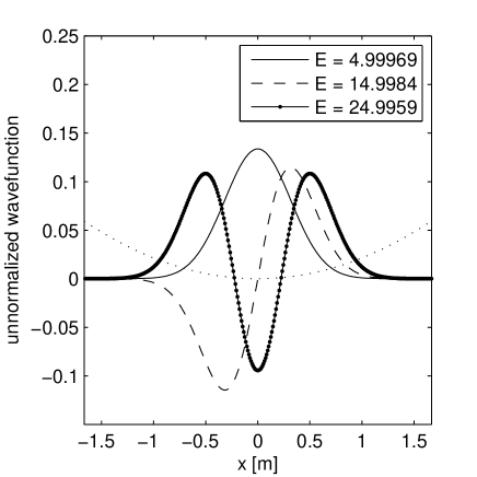
Figure 1: Output of Program 4, which plots the energy eigenfunctions $V(x)$ and a scaled version of the potential $U(x)=1/2\cdot 100\cdot x^{2}$. The corresponding energies displayed within the figure legend, 4.99969, 14.9984 and 24.9959, are, within rounding error, precisely those expected from Eq. (7) for the three lowest-energy modes.

V A Note on Units in our Programs

When doing numerical calculations, it is important to minimize the effect of rounding errors by choosing units such that the variables used in the simulation are of the order of unity. In the programs presented here, our focus being undergraduate physics students, we wanted to avoid unnecessarily complicating matters. To make the equations more familiar to the students, we explicitly left constants such as $\hbar$ in the formulas and chose units such that $\hbar=1$ and $m=1$. We recognize that others may have other opinions on how to address this issue. An alternative approach used in research is to recast the equations in terms of dimensionless variables, for example by rescaling the energy to make it dimensionless by expressing it in terms of some characteristic energy in the problem. In a more advanced course for graduate students or in a course in numerical methods, such is an approach which would be preferable.

VI Time Dependent Phenomena

The separable solutions $|\Psi_{E}(t)\rangle$ are only a subset of all possible solutions of Eq. (1). Fortunately, they are complete set so that we can construct the general solution via the linear superposition

$$|\Psi(t)\rangle=\sum_{E}a_{E}|\Psi_{E}(0)\rangle exp(-iEt/\hbar)$$ (8)

where $a_{E}$ are constants and the sum is over all possible values of $E$. The important difference between the separable solutions (5) and the general solution (8) is that the probability densities derived from the general solutions are time-dependent whereas those derived from the separable solutions are not. A very apt demonstration of this is provided in the Program 5 which calculates the time-dependent probability density $\rho(x,t)$ for a particle trapped in a a pair of finite-square wells whose initial state $|\Psi(0)\rangle$ is set equal to the the equally-weighted superposition

$$|\Psi(0)\rangle=\frac{1}{\sqrt{2}}\left(|\Psi_{E_{0}}\rangle+|\Psi_{E_{1}}\rangle\right)$$ (9)

of the ground state $|\Psi_{E_{0}}\rangle$ and first excited state $|\Psi_{E_{1}}\rangle$ of the double well system. As snapshots of the program output show in Fig. 2, the particle is initially completely localized in the rightmost well. However, due to $E_{0}\neq E_{1}$, the probability density

$$\rho(x,t)=\frac{1}{2}[\;|\psi_{E_{0}}(x)|^{2}\;+\;|\psi_{E_{1}}(x)|^{2}\;\;+\;$$

$$\;2|\psi_{E_{0}}(x)||\psi_{E_{1}}(x)|cos^{2}\left({(E_{1}-E_{2})t}/{\hbar}\right)\;]$$ (10)

is time-dependent, oscillating between the $\rho(x)$ that corresponds to the particle being entirely in the right well

$$\rho(x)=\left|\;|\psi_{E_{0}}(x)|+|\psi_{E_{1}}(x)|\;\right|^{2}$$ (11)

and $\rho(x)$ for the particle being entirely in the left well

$$\rho(x)=\left|\;|\psi_{E_{0}}(x)|-|\psi_{E_{1}}(x)|\;\right|^{2}.$$ (12)

By observing the period with which $\rho(x,t)$ oscillates in the simulation output shown in Fig. 2 students can verify that it is the same as the period of oscillation ${2\pi\hbar}/{(E_{1}-E_{2})}$ expected from Eq. (10).

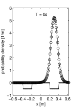
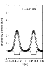
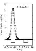
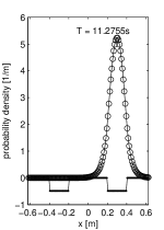
Figure 2: The probability density $\rho(x,t)$ output from Program 5 for a particle trapped in a pair of finite-height square well potentials that are closely adjacent. The initial state of the particle is chosen to be $|\Psi(0)\rangle\sim|E_{0}\rangle+|E_{1}\rangle$. Shown is $\rho(x,t)$ plotted for times $T=\{0,0.25,0.5,0.75,1.0\}\times{2\pi\hbar}/{(E_{1}-E_{2})}$.

%****************************************************************
% Program 5: Calculate Probability Density as a function of time
% for a particle trapped in a double-well potential
%****************************************************************

% Potential due to two square wells of width 2w
% and a distance 2a apart
w = L/50; a = 3*w;
U = -100*( heaviside(x+w-a) - heaviside(x-w-a) ...
                + heaviside(x+w+a) - heaviside(x-w+a));

% Finite-difference representation of Laplacian and Hamiltonian,
% where hbar = m = 1.
e = ones(N,1); Lap = spdiags([e -2*e e],[-1 0 1],N,N)/dx^2;
H = -(1/2)*Lap + spdiags(U,0,N,N);

% Find and sort lowest nmodes eigenvectors and eigenvalues of H
nmodes = 2; options.disp = 0; [V,E] = eigs(H,nmodes,’sa’,options);
[E,ind] = sort(diag(E));% convert E to vector and sort low to high
V = V(:,ind);           % rearrange coresponding eigenvectors
% Rescale eigenvectors so that they are always
% positive at the center of the right well
   for c = 1:nmodes
       V(:,c) = V(:,c)/sign(V((3*N/4),c));
   end

%****************************************************************
% Compute and display normalized prob. density rho(x,T)
%****************************************************************
% Parameters for solving the problem in the interval 0 < T < TF
TF = 10;                  % Length of time interval
NT = 100;                 % No. of time points
T = linspace(0,TF,NT);    % Time vector

% Compute probability normalisation constant (at T=0)
  psi_o = 0.5*V(:,1)+0.5*V(:,2);    % wavefunction at T=0
  sq_norm = psi_o’*psi_o*dx;        % square norm = |<ff|ff>|^2

Usc = U*max(abs(V(:)))/max(abs(U));   % rescale U for plotting

% Compute and display rho(x,T) for each time T
for t=1:NT;    % time index parameter for stepping through loop
  % Compute wavefunction psi(x,T) and rho(x,T) at T=T(t)
  psi = 0.5*V(:,1)*exp(-i*E(1)*T(t)) ...
            + 0.5*V(:,2)*exp(-i*E(2)*T(t));
  rho = conj(psi).*psi/sq_norm;   % normalized probability density

  % Plot rho(x,T) and rescaled potential energy Usc
  plot(x,rho,’o-k’, x, Usc,’.-b’); axis([-L/8 L/8 -1 6]);
  lgnd_str = [repmat(’T = ’,1,1),num2str(T)];
  text(-0.12,5.5,lgnd_str, ’FontSize’, 18);
  xlabel(’x [m]’, ’FontSize’, 24);
  ylabel(’probability density [1/m]’,’FontSize’, 24);

  pause(0.05);                    % wait 0.05 seconds
end

VII Wavepackets and Step Potentials

Wavepackets are another time-dependent phenomenon encountered in undergraduate quantum mechanics for which numerical solution techniques have been typically advocated in the hopes of promoting intuitive acceptance and understanding of approximations necessarily invoked in more formal, analytic treatments. Program 6 calculates and displays the time evolution of a wavepacket for one of two possible potentials, either $U=0$ or a step potential $U=U_{o}\Theta(x-L)$. The initial wavepacket is generated as the Fast Fourier Transform of a Gaussian momentum distribution centered on a particular value of the wavevector $k_{o}$. Because the wavepacket is composed of a distribution of different $k$s, different parts of the wavepacket move with different speeds, which leads to the wave packet spreading out in space as it moves.

While there is a distribution of velocities within the wavepacket, two velocities in particular are useful in characterizing it. The phase velocity $v_{w}=\omega/k=E/p=\hbar k_{o}/2m$ is the velocity of the plane wave component which has wavevector $k_{o}$. The group velocity $v_{g}=\hbar k_{o}/m$ is the velocity with which the expectation value $<x>$ moves and is the same as the classical particle velocity associated with the momentum $p=\hbar k$. Choosing $U=0$, students can modify this program to plot $<x>$ vs $t$. They can extract the group velocity from their numerical simulation and observe that indeed $v_{g}=2v_{w}$ for a typical wave packet. Students can also observe that, while $v_{g}$ matches the particle speed from classical mechanics, the wavepacket spreads out as time elapses.

%****************************************************************
% Program 6: Wavepacket propagation using exponential of H
%****************************************************************
% Parameters for solving the problem in the interval 0 < x < L
L = 100;                        % Interval Length
N = 400;                        % No of points
x = linspace(0,L,N)’;           % Coordinate vector
dx = x(2) - x(1);               % Coordinate step

% Parameters for making intial momentum space wavefunction phi(k)
ko = 2;                      % Peak momentum
a = 20;                      % Momentum width parameter
dk = 2*pi/L;                 % Momentum step
km=N*dk;                     % Momentum limit
k=linspace(0,+km,N)’;        % Momentum vector

% Make psi(x,0) from Gaussian kspace wavefunction phi(k) using
% fast fourier transform :
phi = exp(-a*(k-ko).^2).*exp(-i*6*k.^2); % unnormalized phi(k)
psi = ifft(phi); % multiplies phi by expikx and integrates vs. x
psi = psi/sqrt(psi’*psi*dx);            % normalize the psi(x,0)

% Expectation value of energy; e.g. for the parameters
% chosen above <E> = 2.062.
avgE = phi’*0.5*diag(k.^2,0)*phi*dk/(phi’*phi*dk);

% CHOOSE POTENTIAL U(X): Either U = 0 OR
% U = step potential of height avgE that is located at x=L/2
%U = 0*heaviside(x-(L/2));  % free particle wave packet evolution
U = avgE*heaviside(x-(L/2));    % scattering off step potential

% Finite-difference representation of Laplacian and Hamiltonian
e = ones(N,1); Lap = spdiags([e -2*e e],[-1 0 1],N,N)/dx^2;
H = -(1/2)*Lap + spdiags(U,0,N,N);

% Parameters for computing psi(x,T) at different times 0 < T < TF
NT = 200; ΨΨΨ% No. of time steps
TF = 29; T = linspace(0,TF,NT); % Time vector
dT = T(2)-T(1);ΨΨΨ% Time step
hbar = 1;

% Time displacement operator E=exp(-iHdT/hbar)
E = expm(-i*full(H)*dT/hbar);Ψ% time desplacement operator

%***************************************************************
% Simulate rho(x,T) and plot for each T
%***************************************************************
for t = 1:NT;         % time index for loop
    % calculate probability density rho(x,T)
    psi = E*psi;            % calculate new psi from old psi
    rho = conj(psi).*psi;   % rho(x,T)

    plot(x,rho,’k’);     % plot rho(x,T) vs. x
    axis([0 L 0 0.15]);  % set x,y axis parameters for plotting
    xlabel(’x [m]’, ’FontSize’, 24);
    ylabel(’probability density [1/m]’,’FontSize’, 24);

    pause(0.05);         % pause between each frame displayed
end

% Calculate Reflection probability
R=0;
for a=1:N/2;
    R=R+rho(a);
end
R=R*dx

In Program 6, we propagate the wave function forward via the formal solution

$$|\Psi(t)\rangle=exp(-iHt/\hbar)|\Psi(0)\rangle,$$ (13)

where the Hamiltonian matrix $H$ is in the exponential. This solution is equivalent to Eq. (6), as as can be shown by simple substitution. Moreover, MATLAB has no trouble exponentiating the matrix that numerically representing the Hamiltonian operator as long as the matrix is small enough to fit in the available computer memory.

Even more interestingly, students can use this method to investigate scattering of wavepackets from various potentials, including the step potential $U=U_{o}\Theta(x-L/2)$. In Fig. 3, we show the results of what happens as the wavepacket impinges on the potential barrier. The parameters characterizing the initial wavepacket have been deliberately chosen so that the wings do not fall outside the simulation area and initially also do not overlap the barrier on the right. If $\langle E\rangle\ll U_{o}$, the wavepacket is completely reflected from the barrier. If $\langle E\rangle\approx U_{o}$, a portion of the wave is is reflected and a portion is transmitted through. If $\langle E\rangle~{}\gg U_{o}$, almost all of the wave is transmitted.

Figure 3: Output of Program 6 showing a wavepacket encountering step potential of height $\sim\langle E\rangle$ located at $x/L=0.5$ at different times.

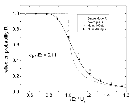
Figure 4: The reflection probability $R$ vs. $\langle E\rangle/U_{o}$. The dashed line is simply Eq. (14) where we subsitute $E=\langle E\rangle$, the solid line is Eq. (14) averaged over the energy distribution in the incident wavepacket, and the points are numerical results obtained using Program 6, where the horizontal distance between points is $\sigma_{E}/U_{o}$ where $\sigma_{E}$ is the standard deviation of the energy distribution in the wavepacket.

In Fig. 4 we compare the reflection probability $R$ calculated numerically using Program 6 with $R$ calculated by averaging the single-mode griffiths expression

$$R(E)=\left|\frac{\sqrt{E}-\sqrt{E-U_{o}}}{\sqrt{E}+\sqrt{E-U_{o}}}\right|^{2}$$ (14)

over the distribution of energies in the initial wavepacket. While the numerically and analytically estimated $R$ are found to agree for large and small $\langle E\rangle/U_{o}$, there is a noticeable discrepancy due to the shortcomings of the numerical simulation for $\langle E\rangle/U_{o}\approx 1$. This discrepancy can be reduced significantly by increasing the number of points in the simulation to 1600 but only at the cost of significantly slowing down the speed of the computation. For our purposes, the importance comparing the analytical and numerical calculations is that it gives student a baseline from which to form an opinion or intuition regarding the accuracy of Eq. (14).

VIII Conclusions

One benefit of incorporating numerical simulation into the teaching of quantum mechanics, as we have mentioned, is the development of student intuition. Another is showing students that non-ideal, real-world problems can be solved using the concepts they learn in the classroom. However, our experimentation incorporating these simulations in quantum physics at WPI during the past year has shown us that the most important benefit is a type of side-effect to doing numerical simulation: the acceptance on an intuitive level by the student that functions are like vectors and differential operators are like matrices. While in the present paper, we have only had sufficient space to present the most illustrative MATLAB codes, our goal is to eventualy make available a more complete set of polished codes is available for downloading either from the authors or directly from the file exchange at MATLAB Central.matlabcentral

References

- (1) P. A. M. Dirac, The Principles of Quantum Mechanics, 1st ed., (Oxford University Press, 1930).
- (2) Born’s law is stated as a proportionality because an additional factor is necessary depending on the units of
- (3) C. C. Silva and R. de Andrade Martins, “Polar and axial vectors versus quaternions,” Am. J. Phys. 70, 958-963 (2002).
- (4) R. W. Robinett, Quantum Mechanics: Classical Results, Modern Systems, and Visualized Examples, (Oxford University Press, 1997).
- (5) H. Gould, “Computational physics and the undergraduate curriculum,” Comput. Phys. Commun. 127, 6–10 (2000); J. Tobochnik and H. Gould, “Teaching computational physics to undergraduates,” in Ann. Rev. Compu. Phys. IX, edited by D. Stauffer (World Scientific, Singapore, 2001), p. 275; H. Gould, J. Tobochnik, W. Christian, An Introduction to Computer Simulation Methods: Applications to Physical Systems, (Benjamin Cummings, Upper Saddle River, NJ, 2006) 3rd ed..
- (6) R. Spenser, “Teaching computational physics as a laboratory sequence,” Am. J. Phys. 73, 151-153 (2005).
- (7) D. Styer, “Common misconceptions regarding quantum mechanics,” Am. J. Phys. 64, 31-34 (1996).
- (8) A. Goldberg, H. M. Schey, J. L. Schwartz, “Computer-Generated Motion Pictures of One-Dimensional Quantum-Mechanical Transmission and Reflection Phenomena,” Am. J. Phys. 35, 177-186 (1967).
- (9) C. Singh, M. Belloni, and W. Christian, “Improving students’ understanding of quantum mechanics,” Physics Today, August 2006, p. 43.
- (10) These MATLAB commands are explained in an extensive on-line, tutorial within MATLAB and which is also independently available on the MATHWORKS website, http://www.mathworks.com/.
- (11) D. J. Griffiths, Introduction to Quantum Mechanics, 2nd Ed., Prentice Hall 2003.
- (12) A. Garcia, Numerical Methods for Physics, 2nd Ed., (Prentice Hall, 1994).
- (13) G. Lindblad, “Quantum Mechanics with MATLAB,” available on internet, http://mathphys.physics.kth.se/schrodinger.html.
- (14) See the user file exchange at http://www.mathworks.com/matlabcentral/.