Optical carrier wave shocking: detection and dispersion

Abstract

Carrier wave shocking is studied using the Pseudo-Spectral Spatial Domain (PSSD) technique. We describe the shock detection diagnostics necessary for this numerical study, and verify them against theoretical shocking predictions for the dispersionless case. These predictions show Carrier Envelope Phase (CEP) and pulse bandwidth sensitivity in the single-cycle regime. The flexible dispersion management offered by PSSD enables us to independently control the linear and nonlinear dispersion. Customized dispersion profiles allow us to analyze the development of both carrier self-steepening and shocks. The results exhibit a marked asymmetry between normal and anomalous dispersion, both in the limits of the shocking regime and in the (near) shocked pulse waveforms. Combining these insights, we offer some suggestions on how carrier shocking (or at least extreme self-steepening) might be realised experimentally.

I Introduction

The self-steepening of an optical pulse envelope was first studied by DeMartini et al. in 1967 DeMartini-TGK-1967pr , and is a well-known phenomenon associated with self-phase modulation (SPM). Surprisingly however, the possibility of self-steepening of the optical carrier wave was considered even earlier in a 1965 paper by Rosen Rosen-1965pr , who showed that, for a third order $\chi^{(3)}$ nonlinearity (and under suitable conditions), a shock (or field discontinuity) develops in a finite distance. This latter phenomenon received little attention for more than 30 years, until it was revisited in the 1990s by Moloney et al. Flesch-PM-1996prl ; Gilles-MV-1999pre , who performed Finite Difference Time Domain (FDTD) simulations of the process. Three dimensional FDTD simulations of carrier shocking have recently been performed by Trillo et al. Trillo-MC-2006ecleo .

In the present paper, we investigate carrier wave shocking in $\chi^{(3)}$ nonlinear materials where SPM is accompanied by the generation of (odd) higher harmonics. For the dispersionless case we have generalized earlier predictions based on the method of characteristics (MOC) to allow for arbitrary initial waveforms. This allows us, for example, to predict the carrier envelope phase (CEP) sensitivity of the shocking distance for optical pulses, as well as the dependence on pulse length.

Our primary interest in this paper is the effect of linear dispersion on carrier shock formation. Since no analytic solutions exist in this case, we are forced to rely on numerical simulations. In any discussion of carrier wave shocking, it is important to distinguish between three related concepts: the physical system, the mathematical model, and the numerical model. The mathematical model is an approximation to the physical system, while the numerical model is an approximation to the mathematical model. Actual discontinuities occur only in the mathematical model, and it is these to which the idea of shock formation refers. In the physical system, discontinuities are prevented by phenomena not included in the mathematics, while numerical codes inevitably fail as a mathematical discontinuity is approached. The indicator of an imminent “shock” is the rapidly increasing gradient (steepening) of the optical carrier. In the numerical model, we see numerical symptoms generated by extreme self-steepening, and these correlate with the onset of the discontinuities in the mathematical model. Under these circumstances, it has been necessary for us to develop a quantitative numerical test of “shock formation”. We have found the most satisfactory diagnostic to be “Local Discontinuity Detection” (LDD), which gives results that are in good agreement with theoretical MOC predictions based on the mathematical model. LDD provides a clear numerical measure of the rapid steepening that precedes the appearance of a discontinuity in the mathematical representation. We continue to use the term “shock” to describe the situation where a mathematical shock is imminent.

In our simulations, we exploit the flexibility in dispersion management offered by the Pseudo-Spectral Spatial Domain (PSSD) technique Tyrrell-KN-2005jmo to study carrier shock formation for a range of simple dispersion profiles, and determine the degree of phase mismatch that carrier shocking can tolerate. As expected, we find that shocking occurs when the nonlinearity dominates the linear dispersion. However, it emerges that the process is asymmetric, with anomalous dispersion being far more conducive to shocking than normal dispersion. Hence, the fact that the LDD scheme does not detect carrier shocks in simulations involving (normally dispersive) fused silica, even at powers equal to its damage threshold, is neither surprising nor necessarily discouraging. After all, anomalously dispersive materials could potentially be engineered. Further, our results also relate to how one might perform carrier shaping (as opposed to carrier steepening), a process that has some interesting applications.

After briefly describing our simulation methods in section II, we consider dispersionless shocking and the method of characteristics in III, and our LDD shock detection scheme in IV. Then we discuss the effect of dispersion on carrier shocking in V, followed by our numerical results in VI. In VII we consider the potential relevance to experimental detection of carrier steepening and/or shocks. Finally, in VIII, we present our conclusions.

II Simulation Methods

The PSSD method Tyrrell-KN-2005jmo ; Fornberg-PSmethods offers significant advantages over the traditional FDTD and Pseudospectral Time-Domain (PSTD) Hagness techniques for modeling the propagation and interaction of few-cycle pulses. Run times are generally faster, and PSSD also offers far greater flexibility in the handling of dispersion. Whereas FDTD and PSTD Hagness propagate fields $E(z),H(z)$ forward in time, PSSD propagates fields $E(t),H(t)$ forward in space. It is important to keep this difference in mind when comparing our results to those in Hagness . Under PSSD, the entire time-history (and therefore frequency content) of the pulse is known at any point in space, so arbitrary dispersion incurs no extra computational penalty. In contrast, the FDTD or PSTD approaches use convolutions incorporating time-response models for dispersion.

We apply the PSSD algorithm to two representations of the field and source-free Maxwell’s equations in non-magnetic media; the first uses the $E$ and $H$ fields, and the second the directional fields $\vec{G}^{\pm}(t)~{}=~{}\alpha_{r}(t)\ast\vec{E}_{x}(t)\pm\beta_{r}\vec{H}_{y}(t)$ Kinsler-RN-2005-flvar . Here the $\alpha_{r}$, $\beta_{r}$ include the (linear) permittivity and permeability of the material (i.e. $\epsilon(t),\mu$). These $G^{\pm}$ fields enable us to rewrite Maxwell’s equations, and efficiently separate out the relevant forward-going part of the field.

For an instantaneous $\chi^{(3)}$ nonlinearity, the equations for $E$ and $H$ in the 1D (plane wave) limit are

$$\frac{dH_{y}(t;z)}{dz} = -\frac{d}{dt}\left[\epsilon_{0}\epsilon_{r}(t)*E_{x}(t;z)+\chi^{(3)}E_{x}(t;z)^{3}\right],$$ (1)

$$\frac{dE_{x}(t;z)}{dz} = -\frac{d}{dt}\left[\mu_{0}H_{y}(t;z)\right].$$ (2)

The $G^{\pm}$ field simulations usually assume $G^{-}=0$, and as a result contain only forward traveling components. The forward-only wave equation for $G^{+}$ is

$$\frac{dG^{+}(t;z)}{dz} = -\frac{d}{dt}\left[\beta_{r}\alpha_{r}(t)*G^{+}(t;z)+\beta_{r}\chi^{(3)}E(t;z)^{3}\right],$$ (3)

where it is most straightforward to calculate the nonlinear term by reconstructing $E(t;z)$ from $G^{+}(t;z)$ in the frequency domain using $\tilde{E}(\omega;z)=\tilde{G}^{+}(\omega;z)/2\tilde{\alpha}_{r}(\omega)$, since $G^{-}=0$. Notice the similarity between eqns. (1) and (3), but that eqn. (3) propagates the field in a single first order equation, rather than two.

Typical array sizes used in pulse simulations were $N=2^{14}$ covering a time window $T=200$fs, and (spatial) propagation steps were $dz=0.4cT/N\approx 0.9$nm. We ensured the stability of our integration using Orszag’s 2/3 rule NumericalRecipes , which involves setting the upper part of the spectral range to zero. It is worth noting that changing this cut-off, either by adjusting its position, or by using a smoothed (rather than step-like) filter, made little difference to test simulations. The pulse profile used as an initial condition was

$$E(t) = E_{0}\sin(\omega_{1}t+\phi){\textrm{ sech}}(0.28\omega_{1}t/\tau),$$ (4)

where our standard parameters were $\omega_{1}=2.356\times 10^{15}$rad/s (i.e. $\lambda=800$nm) with $\tau=0.9\dot{3}$. Such pulses are rather short (since the number of cycles inside the intensity FWHM is $\tau$), but in fact the shocking distance is only weakly dependent on the pulse width, with significant variation only appearing for pulses of a few cycles or less.

We also performed CW simulations, for which we modeled just a single cycle of the carrier. assisted by the periodic nature of the discrete Fourier transform. For these we used array sizes of $N=2^{10}$, and the time window was set by the period of the field oscillations.

Our default value of nonlinear strength was $\chi^{(3)}E_{0}^{2}=0.02$, which is comparable to that in fused silica at an intensity of $0.7\times 10^{14}$ W/cm²; our $\chi^{(3)}$ parameter is equivalent to $\eta$ in Rosen Rosen-1965pr , and $a$ in Gilles et al.Gilles-MV-1999pre . We use an instantaneous nonlinearity, since our primary interest is linear dispersion, and that is a far more significant effect than the nonlinear time response.

III Carrier Wave Shocking

As an introduction to the process of carrier wave shocking, fig. 1 shows the profile of a pulse propagating in a dispersionless $\chi^{(3)}$ medium, just before a shock occurs. The nonlinearity gives rise to a nonlinear index of refraction $n_{2}E^{2}$, the effect of which is to increase the effective refractive index in the more intense regions of the profile. This reduces the phase velocity at the peak of each oscillation with respect to the rest of the waveform, and causes the slope on the trailing edges to increase dramatically.

Figure 1: The profile of a few-cycle optical pulse just prior to shocking in the dispersionless limit. The larger oscillations in the centre of the pulse undergo more self-steepening than those in the wings. The standard pulse parameters were used.

The effects seen in fig. 1 are associated with the generation of third and higher harmonics, although the harmonic components are not particularly strong even when a shock is about to occur. As an example, fig. 2 shows how the harmonics build up as shocking is approached. The $\omega^{4}$ scaling of the intensity spectrum in the figure exaggerates the contribution of the higher orders, and has been chosen for illustrative purposes. Notice that the profile becomes nearly flat (i.e. the spectrum falls off as the 4th power of the frequency) just before shocking is registered at around 4.3$\mu$m.

Figure 2: Development of the heights of the scaled harmonic peaks as a pulse approaches the (LDD) shocking distance of 4.3$\mu$m in the dispersionless case. Each line perpendicular to the $\omega/\omega_{1}$ axis corresponds to the (scaled) contribution from that spectral peak. Note that the viewpoint has been rotated so that the contribution from the fundamental is to the right. The initial pulse contained about 33 cycles ($\tau=33$).

If we write

$$E = A(t)\left[\sin(\omega_{1}t)+\gamma\cos(3\omega_{1}t+\psi)\right],$$ (5)

we find that an appropriate choice of $A(t)$, with $\gamma=0.1$ and $\psi=0$, gives us a passable match to fig. 1. Note that this choice of $\psi$ corresponds to the phase of third harmonic generation (THG) under index matched conditions, i.e. where $n_{0}=n(\omega_{1})=n(\omega_{3})$.

Rosen’s original paper Rosen-1965pr used the MOC to predict the formation of a value discontinuity in the field at certain points within the profile. If the displacement of the dispersionless medium is written

$$D = \epsilon_{0}\left(E+\chi^{(1)}E+\chi^{(3)}E^{3}\right),$$ (6)

he showed that the wave equation for $E$ is

$$c^{2}\frac{\partial^{2}E}{\partial x^{2}} = \left(1+\chi^{(1)}\right)\frac{\partial^{2}E}{\partial t^{2}}+\chi^{(3)}\frac{\partial^{2}E^{3}}{\partial t^{2}},$$ (7)

and that the associated equation governing the characteristic lines of $E$ is

$$\frac{\partial E}{\partial t}+v(E)\frac{\partial E}{\partial x} = 0.$$ (8)

Here, the velocity $v(E)$ is given by

$$v(E) = \frac{c}{(\epsilon_{r}+3\chi^{(3)}E^{2})^{1/2}},$$ (9)

where $\epsilon_{r}=1+\chi^{(1)}={n_{0}}^{2}$ is the (relative) dielectric constant and $n_{0}$ the linear refractive index.

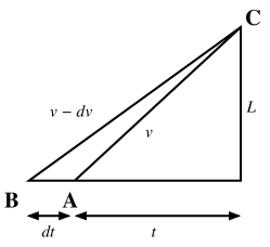
Figure 3: Method of Characteristics. Two points A and B on the field profile, separated initially by a time difference $dt$ travel at different speeds $v-dv$ and $v$, and meet at point C.

Using eqn. (9) along with the construction shown in fig. 3, we can derive a simple formula for the distance to shocking. The figure shows two characteristics AC and BC, originating from points A and B, and converging towards a shock at C after a distance of $L$. The intensity at A is higher than at B, so the speed associated with AC (represented by its gradient) is lower than that of BC. This means that at C, the field has two values, and a discontinuity has formed. From the geometry of the figure, it is easy to show that

$$\frac{dv}{dt} = \frac{v}{t}=\frac{v^{2}}{L}=\frac{(c/n_{0})^{2}}{L},$$ (10)

where $t$, $v=c/n_{0}$, and $L=vt$ are respectively time, speed and distance.

On the other hand, differentiating eqn. (9) leads to

$$\frac{dv}{dt} = -\frac{3c\chi^{(3)}}{2\left(n_{o}^{2}+3\chi^{(3)}E^{2}\right)^{3/2}}\frac{d\left(E^{2}\right)}{dt},$$ (11)

and this combined with eqn. (10) yields

$$L = \frac{cn_{0}\sqrt{1+3\chi^{(3)}E^{2}/n_{o}^{2}}}{3\chi^{(3)}(-dE^{2}/dt)}$$ (12)

$$= \frac{c}{4n_{2}}\frac{\sqrt{1+8n_{2}E^{2}/n_{o}}}{(-dE^{2}/dt)},$$ (13)

where $n_{2}=3\chi^{(3)}/8n_{o}$ is the material parameter determining the intensity induced refractive index shift as $n_{2}E^{2}$. For a given profile, a shock will occur first at the point where $-dE^{2}/dt$ reaches its negative extremum. We can therefore define the shocking distance as

$$L_{shock} = \frac{c}{4n_{2}}Min{\frac{\sqrt{1+8n_{2}E^{2}/n_{o}}}{(-dE^{2}/dt)}}$$ (14)

$$\simeq \frac{c}{4n_{2}}Min{\frac{1}{(-dE^{2}/dt)}}~{}~{}~{}~{}\textrm{for}~{}~{}~{}~{}8n_{2}E^{2}/n_{o}\ll 1.~{}~{}~{}~{}$$ (15)

This formula is more general than that of either Rosen Rosen-1965pr or Gilles et al. Gilles-MV-1999pre . Notice in particular that the parameter that controls the shock behaviour is not the gradient of the field ($dE/dt$), but that of the field squared ($dE^{2}/dt$).

For a sinusoidal initial waveform $E=E_{0}\sin(\omega_{1}t+\phi)$, it is easy to show that shocks form at

$$\omega_{1}t = -\pi/4+j\pi-\phi,$$ (16)

where $j$ is an integer, and that the shocking distance is

$$L_{shock} = \frac{2cn_{0}}{3\omega_{1}\chi^{(3)}E_{0}^{2}}~{}~{}~{}~{}=\frac{c}{4\omega_{1}n_{2}E_{0}^{2}}.$$ (17)

The approach is readily extended to pulsed waveforms of the type defined in eqn. (4). Analytical results can be derived in the new situation in which eqn. (16) becomes a transcendental equation. However, the results are cumbersome and it is simpler to scan the profile numerically to determine the shocking parameters. It turns out that the shocking distance for short pulses exhibits an interesting sensitivity to the carrier envelope phase $\phi$. Whilst in the CW case all locations defined by eqn. (16) were equivalent, for pulses, the one nearest the peak of the envelope has a shorter $L_{shock}$ than the others.

A set of results is displayed in fig. 4 where the shocking distance is plotted as a function of the carrier phase $\phi$ for sech profiles with different pulse widths $\tau$. The dotted line is for the case of a very broad pulse for which $L_{shock}$ is given by eqn. (17). The sharp peaks mark a curve crossings where the shock location switches from one point on the sinusoid to another. Notice that the range of shocking distances increases for shorter pulses, and that, unsurprisingly, the lowest values occur when $\phi$ is around $\pi/2$ i.e. when the pulse has a cosine form.

One very important point to note from fig. 4 is that for pulses containing more than a few cycles, the dependence of the shocking distance on pulse width is very weak. We will see this message repeated later in section V, with shock regions being similar for both single cycle ($\tau=1$) pulses and CW ($\tau=\infty$) fields.

Figure 4: MOC shocking distances as a function of phase, for pulses as in eqn. (4), allowing for different pulse lengths. We include the 1/2 cycle $\tau=0.56$ results to emphasize the trend; but even for a long pulse ($\tau=28$), a small peak can be seen just below $\phi/\pi=0.01$. The peak position is weakly $\tau$ dependent. The $+$ signs denote LDD shocking distances obtained from simulations of the $\tau=0.9\dot{3}$ case.

IV Shock Detection

Since optical shock formation is directly associated with regions of increasingly steep field gradient, any numerical scheme, however sophisticated, is bound to fail at some point in the process. We therefore want to recognize when a shock is imminent, not only to avoid numerical problems, but as a means to estimate the distance at which a discontinuity would occur in the mathematical model.

One obvious symptom of impending numerical failure is loss of energy conservation Tyrrell-KN-2005jmo . However, this does not give an indication at the first instance of a shock forming, but rather signals the accumulated effect of multiple small numerical failures from many shocked regions.

A more physical strategy is to search for regions where the field gradient $dE/dt$ is large and increasing rapidly, and to use this to predict the shocking point. A useful variant, suggested by the MOC calculation in the previous section, is to use the value of $-dE^{2}/dt$ instead of the gradient.

Overall, we find that the best method is Local Discontinuity Detection (LDD), which is similar to techniques used in other fields (see e.g. PagendarmSeitz-1993 ). As the shock regime is approached, narrow shoulders with associated points of inflection appear within the regions of rapidly increasing gradient. The procedure is therefore to scan the field profile for the maximum gradient (of either $E$ or $E^{2}$) and, if it occurs near a point of inflection, an incipient shock is registered. An example of a pulse that has just triggered the LDD diagnostic is shown in fig 5.

The LDD method requires two parameters. The first determines the time scale used in determining whether a point of inflection exists. For this, we pick the scale set by our temporal grid and insist that the field gradients calculated at three adjacent grid points have opposing signs: either up-down-up, or down-up-down. The second determines the maximum range allowed between the maximum gradient and the point of inflection, and our default value for this was 10 grid points. In our simulations, we see that the position of the first detected shock depends only weakly on this range. We can easily minimize the small sensitivity to these parameters by holding them fixed throughout any given set of simulations. As a result, we have found LDD to be a sensitive and reliable method of shock detection.

Figure 5: The profile of a few-cycle optical pulse at the point of shocking. The larger oscillations in the centre of the pulse undergo more self-steepening than those in the wings. (a) The whole pulse, with the LDD carrier shock circled ($\circ$). (b) An expanded view of the shock region, with its point of inflection (at $\sim 9.3$fs) being very close to the steepest gradient (at $\sim 9.1$fs). The standard pulse parameters were used.

Eqn. (17) predicts that the shocking distance should increase linearly with the refractive index $n_{0}$. We use this to test the LDD diagnostic in fig. 6, where the analytical formula is compared with the results of numerical simulations. This figure shows close agreement between prediction (using eqn. (15)) and simulation, where the approximation causes the MOC prediction to be reduced by less than 0.1$\mu$m at $n_{0}=1$. We see similar agreement between simulations using the LDD method and the carrier phase sensitivity shown in fig. 4. The presence of small systematic differences (as on e.g. fig. 4, 6) can be easily understood, since the LDD diagnostic is (strictly speaking) a test of the numerics, and is not a direct test for the presence of a physical shock or mathematical discontinuity.

Figure 6: The LDD shocking distance as a function of refractive index, comparing the approximate MOC prediction from eqn. (15) to PSSD simulations ($+$) for pulses with $\tau=0.9\dot{3}$. Other PSSD simulation results from independent codes give very similar results to those shown on the graph.

V The effect of dispersion on shocking

The primary purpose of this paper is to understand the principles of carrier shock formation in the presence of dispersion. Some simple ideas about the role of dispersion can be understood from eqn.(5) using the insight from eqns.(10) – (15), i.e. that the rate of change of $E^{2}$ is the critical factor in shock development, rather than that of $E$. If only the fundamental and third harmonic components are considered (as in eqn.(5)), the effective refractive indices are

$$\Delta n_{NL:1} = n_{1}+n_{2}\left(1+3\gamma^{2}\right)I_{1},$$ (18)

$$\Delta n_{NL:3} = n_{3}+n_{2}\left(3+\gamma^{2}\right)I_{1}.$$ (19)

Evidently, the relative phase velocity of the two waves is affected by both linear and nonlinear dispersion, so the phase $\psi$ in eqn.(5) will vary accordingly as the pulse propagates. Fig. 7, which shows how $dE^{2}/dt$ varies with $\psi$, suggests that shocking is likely to be exacerbated when $\psi$ is small and positive, but moderated when $\psi$ is negative. Broadly speaking, the former case will be promoted by anomalous dispersion and the latter by normal dispersion; however, the process is clearly complicated, since it involves time-dependent phase shifts between the waves and the interplay of linear and nonlinear dispersion. Of course, since carrier shocking relies on the establishment and maintenance of specific phase relationships between a set of harmonics, it must be expected that strong dispersion of either sign will disrupt the shock formation process. On the other hand, the simple argument that has been offered suggests that shocking may be tolerant to a degree of anomalous dispersion, but not to a similar amount of normal dispersion. In general, therefore, a graph of shocking signature versus refractive index mismatch might be expected to exhibit a shock region where nonlinearity dominates dispersion (displaced in the direction of anomalous dispersion), surrounded by a shock-free region where dispersion dominates the nonlinearity. Moreover, if a dominant coherence length $L_{C}$ can be defined, it is reasonable to expect shocking to occur when this exceeds the characteristic SPM length ($L_{SPM}$). As we shall see, all these features are borne out by the numerical results.

Figure 7: The effect of different time-lags between fundamental and third harmonic on the steepness of the pulse. The field profile is as in eqn. (5), with $A(t)=A_{0}$ and $\gamma=1/16$. (a) Scaled maximum values of $M_{j}=\textrm{Max}(dE^{j}/dt)$ as a function of third harmonic phase offset $\psi$. We can see that the maxima of $dE/dt$ and $dE^{2}/dt$ occur at different $\psi$. (b) Position on the pulse $\theta_{j}=\omega_{1}t_{j}$ of the maxima plotted in the top frame. Note that the kinks in (a) and (b) occur for offsets that give the longest shocking distances, not the shortest.

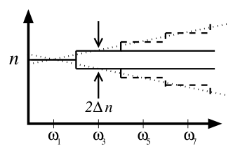
Figure 8: Types of refractive index profile used. The solid lines show a single refractive index step midway between $\omega_{1}$ and $\omega_{3}$, so that the fundamental is always phase mismatched from its higher harmonics, although they remain perfectly phase matched with each other. The dashed lines show multiple refractive index steps, each of the same size, and always midway between subsequent harmonics. The dotted lines show a linear refractive index gradient which gives the same mismatch between subsequent harmonics as the multi-stepped case. We do not show lines for the case of a single step at $4\omega_{1}$ to avoid cluttering the figure.

In our numerical simulations, we make extensive use of model dispersion curves, which enable refractive index differences between harmonics to be freely controlled, and lead to uncomplicated boundaries between the shock and no-shock regimes. The dispersion profiles shown in fig. 8 duly contain either refractive index steps $\Delta n$ at the midpoints between successive odd harmonics, or smooth gradients $\delta$ that provide a similar net change. In the simplest option, there is a single step at $2\omega_{1}$, in which case the dominant coherence length is clearly $L_{C}=\pi/\left|k_{3}-3k_{1}\right|=\pi c/3\omega_{1}\left|n_{3}-n_{1}\right|$; we have also tried a single step at $4\omega_{1}$, which has a shorter $L_{C}$. In all cases, when $n$ increases with frequency, the situation corresponds broadly to normal dispersion, while decreasing $n$ corresponds to anomalous dispersion. The step size (or gradient) is chosen to be comparable to values in fused silica at $\omega_{1}=1.5$rad/fs, where the refractive index differences between the lower harmonics are $\Delta n_{1,3}\approx 0.06$ and $\Delta n_{3,5}\approx 0.12$Gilles-MV-1999pre . While we consider the case of fused silica itself in Section VII, the results based on the model dispersion characteristics are invaluable for understanding the essential principles of carrier shock formation in dispersive media.

VI Results and discussion

We will now analyze our numerical simulations of carrier shocking in the presence of dispersion on the basis of the principles discussed above. Results are included for both a CW wave and for a single-cycle pulse. The CW case gives slightly wider shocking regions, but the differences are minor. This is because the effect of the pulse envelope on the field amplitudes and gradients of the central carrier oscillation is small, except when considering sub-cycle pulses. In the results we present, the energy conservation and LDD measures reveal the presence of sharp boundaries between the shocking and non-shocking regions.

Figure 9: Carrier shocking for CW and pulsed ($\tau=0.9\dot{3}$) cases with a single refractive index step at $2\omega_{1}$. Frame (a) compares chirped pulses at a 40$\mu$m propagation distance from the non-shock region immediately outside of the shocked region; the upper curve (X) is for the negative step, the lower (Y) for the positive step. Frame (b) shows the correlation in the region where $L_{C}\lesssim L_{SPM}$ between energy conservation failure (logarithmic right hand scale, dots) and the LDD detected shocking distance (left hand scale, solid line). The dotted line shows the LDD results for a CW field ($\tau=\infty$).

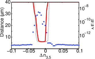
Figure 10: Carrier shocking for CW and pulsed ($\tau=0.9\dot{3}$) cases with a single refractive index step at $4\omega_{1}$; showing the correlation in the region where $L_{C}\lesssim L_{SPM}$ between energy conservation failure (logarithmic right hand scale, dots) and the LDD detected shocking distance (left hand scale, solid line). The dotted line shows the LDD results for a CW field ($\tau=\infty$).

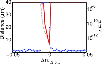
Figure 11: Carrier shocking for CW and pulsed ($\tau=0.9\dot{3}$) cases with multiple refractive index steps; showing the correlation in the region where $L_{C}\lesssim L_{SPM}$ between energy conservation failure (logarithmic right hand scale, dots) and the LDD detected shocking distance (left hand scale, solid line). Note the narrower range of $\Delta n$ as compared to the previous two graphs. The dotted line shows the LDD results for a CW field ($\tau=\infty$).

Results for single refractive index steps at $2\omega_{1}$ and $4\omega_{1}$ are presented in figs. 9 and 10 respectively, whereas fig. 11 has a step midway between all harmonics. In both single stepped cases, a useful coherence length can be defined on the basis of the mismatch between the fundamental and the harmonic just above the step. In the multi-stepped case, there is no easy way to define a dominant coherence length.

Fig. 9(a) shows the pulse profiles in the anomalous (negative) and normal (positive) single step cases, for the smallest step size at which shocking did not occur. The first obvious difference between the profiles is the opposite walk-off direction of the third harmonic, although the third harmonic contribution is hard to see in the anomalous case. The second is that the pulse profiles exhibit distinctly different characteristics according to the sign of the dispersion. Narrow spikes are visible in the anomalous case, whereas profiles with more rounded maxima occur for normal dispersion. A possible interpretation is suggested by fig. 7, where we saw that anomalous dispersion tends to create regions of higher gradient.

The shocking region in fig. 10 has a similar outline to that of fig. 9(b) except that it is slightly narrower, as expected from the coherence length discussion above. However, the shocking region in fig. 11 is much narrower, especially given the change in the $\Delta n$ scale. This is because the multi-stepped nature of the refractive index leads to a correspondingly large range of coherence lengths, with shorter ones corresponding to those spanning several steps. Since the shocking region in the multi-step case has reduced in size by a factor of two or three, a reasonable inference might be that the dominant coherence length results from interaction over two or three refractive index steps.

In realistic media, the refractive index will vary smoothly with frequency, and the group velocity can different from the phase velocity. We can approximate this situation most simply using a refractive index gradient rather than a series of steps. The results using the LDD method in this case can be seen on fig. 12, where now we also vary the strength of the nonlinearity. As in the previous cases, we see a well defined shocking regime that is asymmetric about the non-dispersive case.

Detailed examination shows that the curves in fig. 12 exhibit a marked similarity, and can be brought into near perfect coincidence by applying the scaling $\chi^{(3)}\rightarrow\chi^{(3)}/m$, $L\rightarrow mL$, and $\Delta n\rightarrow\Delta n/m$. We also get a comparable similarity for each of figs. 9,10,11, when simulations at nonlinear strengths of $\chi^{(3)}E_{0}^{2}=0.01$ and $0.04$ are added to the results. This demonstrates that the character of the shocking is dominated by the sign of inter-harmonic phase velocity differences, not by the local group velocity dispersion at each harmonic. Thus anomalous (normal) dispersion is primarily interesting because it gives a negative (positive) refractive index shift between successive harmonics. We leave the complicated (and far more subtle) effects of group velocity differences or dispersion for later work.

Figure 12: Shocking distance vs mismatch for weak refractive index gradients $\delta$, and a range of nonlinearities. This shows an abrupt cut-off at positive $\Delta n$, but a relatively gradual one at negative $\Delta n$. The initial pulses are identical to those in fig. 9. No CW results are shown, since the dispersion experienced by the field would be identical to the multi-stepped case shown in fig. 11.

An important feature of all the results is the pronounced asymmetry, with shocking persisting much further into the anomalous dispersion regime; we have even seen it for the case of a weakly parabolic refractive index.

We can quantify this asymmetry by considering linear and nonlinear contributions to the phase matching of the harmonics (i.e. linear and nonlinear refractive index shifts), as described at the beginning of section V. In the simple single step case shown on fig. 9(b), the 1st–3rd harmonic phase shift will dominate, because it applies to the two most intense spectral components. We can calculate the SPM-induced refractive index shift between the fundamental and third harmonic with eqns. (18) and (19) to be $\Delta n_{NL:1}-\Delta n_{NL:3}=-0.011$, since $\chi^{(3)}E^{2}=0.02$ at the peak of the carrier oscillations, the refractive index is $n_{0}^{2}=2$, and $2n_{2}E_{1}^{2}=2\times 3\chi^{(3)}E^{2}/8n_{0}$. This is roughly comparable to the offset of the shocking region, which is centred at about $\Delta n_{1,3}\simeq-0.014$. We cannot expect perfect agreement, since the calculations ignore the role of higher harmonic generation and depletion of the fundamental. Whilst a simple calculation is reasonably successful in this single-step case, it cannot be applied for a realistic medium – or indeed to the situation shown in fig. 12. There, the effects of dispersion, higher harmonic generation, and nonlinear refractive index shifts are inextricably intertwined.

To summarize, we have demonstrated that shocking is strongly dependent on the interplay between $L_{C}$ and $L_{SPM}$, with shorter $L_{C}$’s (increasing $\Delta n$’s) decreasing the likelihood of shocking. We have also deduced the reasons for the strong asymmetry of the shocking region.

VII Applications and experiments

In sections I and IV, we discussed how imminent carrier shocking might be recognised computationally. In considering whether shocking might be detectable experimentally, we must now decide how it might manifest itself in the laboratory. A mathematical discontinuity is clearly not a physical possibility, even if Rosen Rosen-1965pr did manage to accommodate it theoretically, albiet at the expense of energy conservation. In practice, the increasing field gradients (and spectral broadening) that precede a shock will inevitably engender new physical processes that will limit the steepening. Indeed, we have already seen this happening in the previous two sections, where dispersion has been seen to frustrate the self-steepening process; the next barrier would be the time-scale of the nonlinear response.

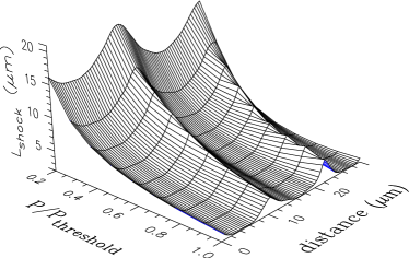
Figure 13: Numerically predicted shocking distances $L_{shock}$ in fused silica. These are the MOC predicted distances for the waveform, assuming the dispersion was (abruptly) neglected, the shortest distance shown is about 1.9$\mu$m. The damage threshold for fused silica was taken to be $P_{threshold}=50$TW/cm².

Although there is no question of a mathematical discontinuity being observed in an experiment, the recent advances in the measurment of optical pulse profiles (see e.g. Goulielmakis-UKBYSWKHDK-2004sci ), suggest that it might be possible to observe carrier steepening. Indeed, it has already been predicted Gilles-MV-1999pre that noticeable steepening effects could occur for pulses propagating in fused silica. Unfortunately, in our own simulations of this process, the LDD shock detection was not triggered at any realistic pulse intensity. Although visible steeping did occur, at no point was a seriously distorted waveform approached, and the effects would have been milder if we had included the finite response time of the nonlinearity. The results presented in fig. 13 show the steepest gradient recorded as a function of distance and pulse intensity for these simulations. The third harmonic coherence length for these parameters is about 7$\mu$m, and we can attribute the regular variation with distance seen in the figure to the third harmonic component aligning with successive oscillations of the fundamental as the waves move across each other. The key reason why incipient shocking was not detected is because the pulse frequency lies in a region of weak normal dispersion, whereas we have shown in section V that a region of weak anomalous dispersion (assuming it could be achieved) would be favourable.

The current interest in media with tailored dispersion characteristics PhotonicBandgapMaterials ; PhotonicCrystals ; MicrostructuredFibres raises the interesting question of whether it might be possible to engineer a material that maximize self-steepening. A major stumbling block would be the need for control over many harmonic orders; however, for a narrow-band pulse, only the dispersion characteristics close to the harmonics would be relevant, which might perhaps make the technical challenge less formidable.

The recognition that dispersion control can enhance (or reduce) carrier self-steepening suggests other applications if we widen our horizons to encompass the more general idea of carrier shaping. In this case, we would exploit both nonlinearity and dispersion control to optimize the shape of the carrier oscillations for a particular experiment. Applications such as high harmonic generation (e.g. Christov-MK-1997prl ) might well benefit from suitably designed carrier wave modulation.

VIII Conclusions

In this paper we have investigated carrier shock formation, developed criteria for detecting its onset in numerical simulations, and shown how it is influenced by a range of parameters, particularly dispersion. We have also obtained remarkable agreement between numerical simulations and theoretical predictions of the shocking distance in the dispersionless limit, and shown that the process is sensitive to both CEP and pulse duration.

Although we have confirmed that shocking occurs in a narrow parameter range, this is far from being the whole picture. In particular, there is a distinct asymmetry between the anomalous and normal dispersion regimes. The former leads to shocking signatures such as the appearance of narrow spikes as the higher harmonics interfere on the steepening part of the pulse profile. In contrast, normal dispersion creates no such features, and the pulse profiles have a rather blunt appearance. The asymmetry arises from the effect of the nonlinear refractive index on the dispersion induced phase mismatch.

The conclusion to be drawn from our results is clear: if they could be engineered, materials with wide regions of weakly anomalous dispersion are much better candidates for generating steep, shock-like field profiles than those (such as silica) with a weak normal dispersion. Detecting incipient shock formation in materials like fused silica is likely to be a near impossible task, given the constraints imposed by their damage thresholds.

References

- (1) F. DeMartini, C.H. Townes, T.K. Gustafson, P.L. Kelly, Phys. Rev. 164, 312 (1967).
- (2) G. Rosen, Phys. Rev. 139, A539 (1965).
- (3) R.G. Flesch, A. Pushkarev, and J.V. Moloney, Phys. Rev. Lett. 76, 2488 (1996).
- (4) L. Gilles, J.V. Moloney, and L. Vázquez, Phys. Rev. E 60, 1051 (1999).
- (5) S.Trillo, G. Millot, C. Conti, ECLEO 2006, paper EB1-05-Mon.
- (6) A. M. Kamchatnov, R. A. Kraenkel, B. A. Umarov, Physi. Rev. E66, 036609 (2002).
- (7) J.C.A. Tyrrell, P. Kinsler, G.H.C. New, J.Mod.Opt. 52, 973 (2005).
- (8) B. Fornberg, “A Practical Guide to Pseudospectral Methods”, Cambridge University Press (1996).
- (9) L. Gilles, S.C. Hagness, and L. Vázquez, J. Comp.Phys. 161 379 (2000).
- (10) P. Kinsler, S.B.P. Radnor, G.H.C. New, Phys. Rev. A. 72, 063807 (2005).
- (11) “Numerical Recipes in C”, W.H. Press et al., (CUP, 1992).
- (12) H.-G.Pagendarm, B.Seitz, in “Scientific Visualization - Advanced Software Techniques” (EllisHorwood 1993), p159.
- (13) E. Goulielmakis, M. Uiberacker, R. Kienberger, A. Baltuska, V. Yakovlev, A. Scrinzi, Th. Westerwalbesloh, U. Kleineberg, U. Heinzmann, M. Drescher, F. Krausz Science 305, 1267 (2004).
- (14) Photonic Bandgap Materials, (Ed: C. M. Soukoulis), (Kluwer, Dordrecht, The Netherlands 1996).
- (15) Photonic Crystals, (Eds: J. D. Joannopoulos, R. D. Meade, J. N. Winn), (Princeton Academic Press, Princeton, NJ 1995).
- (16) J.K. Ranka, R.S. Windeler, A.J. Stentz, Opt. Lett. 25, 25-27 (2000).
- (17) I.P. Christov, M.M. Murnane, H.C. Kapteyn, Phys. Rev. Lett. 78, 1251 (1997).