Kinetic Theory for Binary Granular Mixtures at Low-Density

Many features of granular media can be modelled as a fluid of hard spheres with inelastic collisions. Under rapid flow conditions, the macroscopic behavior of grains can be described through hydrodynamic equations. At low-density, a fundamental basis for the derivation of the hydrodynamic equations and explicit expressions for the transport coefficients appearing in them is provided by the Boltzmann kinetic theory conveniently modified to account for inelastic binary collisions. The goal of this chapter is to give an overview of the recent advances made for binary granular gases by using kinetic theory tools. Some of the results presented here cover aspects such as transport properties, energy nonequipartition, instabilities, segregation or mixing, non-Newtonian behavior, …. In addition, comparison of the analytical results with those obtained from Monte Carlo and molecular dynamics simulations is also carried out, showing the reliability of kinetic theory to describe granular flows even for strong dissipation.

1 Introduction

Granular systems have attracted the attention of the physics community in the past few years, in part because the behavior of these systems under many conditions exhibit a great similarity to ordinary fluids H83 . These conditions include rapid, dilute flows where the dominant transfer of momentum and energy is through binary collisions of the grains. The main difference from ordinary fluids is the absence of energy conservation, leading to both obvious and subtle modifications of the usual macroscopic balance equations as well as the constitutive equations for the irreversible fluxes. However, in spite of the utility of hydrodynamics to describe rapid granular flows, there are still some open questions about its domain of validity and the associated constitutive equations appearing in the hydrodynamic equations K99 .

To isolate the effects of such collisional dissipation from other important properties of granular media, an idealized microscopic model system is usually considered: a system composed by smooth hard spheres with inelastic collisions. As in the elastic case, the collisions are specified in terms of the change in relative velocity at contact but with a decrease in the magnitude of the normal component measured by a positive coefficient of restitution $\alpha\leq 1$. This parameter distinguishes the granular fluid ($\alpha<1$) from the ordinary fluid ($\alpha=1$). Given that the hard sphere system with elastic collisions has been widely studied for both equilibrium and non-equilibrium statistical mechanics HM86 , it is tempting to apply the same methods for the case of inelastic collisions. However, some care is warranted in translating properties of ordinary fluids to granular fluids. In this presentation, a kinetic theory description based on the Boltzmann kinetic equation (which applies at sufficiently low density) will be considered as the appropriate tool to study granular flows from a microscopic point of view.

Although many efforts have been devoted in the past few years to the understanding of granular fluids, the derivation of the form of the constitutive equations with explicit expressions for the transport coefficients is still a subject of interest and controversy. The conditions to obtain a hydrodynamic description are expected to be similar to those for normal fluids. For a given initial state there are two stages of evolution. First, during the kinetic stage there is rapid velocity relaxation to a “universal” velocity distribution that depends on the average local density, temperature, and flow velocity. Subsequently, the hydrodynamic stage is described through a slower evolution of these local hydrodynamic fields as they approach uniformity. The solution to the Boltzmann equation in this second stage is said to be normal, where all space and time dependence of the distribution function occurs through the macroscopic hydrodynamic fields. The Chapman–Enskog method CC70 provides a constructive means to obtain an approximation to such a solution for states whose spatial gradients are not too large. In this case, the explicit form of this normal solution is given as a perturbation expansion in the spatial gradients of the fields. This solution is then used to evaluate the fluxes in the macroscopic balance equations in terms of these gradients. To lowest order the balance equations become the granular Euler equations while to second order they are the granular Navier–Stokes equations. In carrying out this analysis, explicit forms for the transport coefficients are obtained as functions of the coefficient of restitution and other parameters of the collision operator. In this general context, the study of hydrodynamics for granular gases is the same as that for ordinary fluids.

The derivation of hydrodynamics from the inelastic Boltzmann equation has been widely covered in the case of a monodisperse gas where the particles are of the same mass and size. As for elastic collisions, the transport coefficients are given in terms of the solutions of linear integral equations BDKS98 ; BC01 , which are approximately solved by using Sonine polynomial expansions. The estimates for the transport coefficients provided by the Sonine solution compare in general quite well with both direct Monte Carlo simulation (DSMC) of the Boltzmann equation and molecular dynamics (MD) simulation of the gas, even for relatively strong degrees of dissipation BRC99 ; BRCG00 ; BM04 ; MSG05 . This good agreement supports the formal theoretical analysis and the claim that hydrodynamics is not limited to nearly elastic particles D99 ; D02 ; G03 .

Nevertheless, a real granular system is generally characterized by some degrees of polydispersity in density and size, which leads to phenomena very often observed in nature and experiments, such as separation or segregation. Needless to say, the study of granular mixtures is much more complicated than for a monodisperse gas since not only the number of transport coefficients in a multicomponent system is higher than that of a single gas, but also they depend on parameters such as masses, sizes, composition as well as several independent coefficients of restitution $\alpha_{ij}$. Due to these difficulties, studies for multicomponent gases are more scarce in the literature. Many of the previous attempts JM89 to derive hydrodynamics from kinetic theory were carried out in the quasi-elastic limit where the equipartition of energy can be considered as an acceptable assumption. In addition, according to this level of approximation, the inelasticity is only accounted for by the presence of a sink term in the energy balance equation, so that the expressions for the transport coefficients are the same as those obtained for ordinary fluids. However, the theoretical prediction of the failure of energy equipartition in multicomponent granular gases GD99 has been confirmed by computer simulations computer , and even observed in real experiments exp .

Although the possibility of nonequipartition was already pointed out many years ago JM87 , it has not been until recently that a systematic study of the effect of nonequipartition on the Navier–Stokes hydrodynamic equations has been carefuly carried out GD02 ; GMD06 . These new equations and associated transport coefficients provide a somewhat more stringent test of the analysis since the parameter space is much larger. As in the monodisperse case, explicit expressions for the transport coefficients requires also to consider Sonine polynomial expansions. The numerical accuracy of this Sonine expansion has been confirmed by comparison with Monte Carlo simulations of the Boltzmann equation in the cases of the shear viscosity MG03 and the tracer diffusion GM04 coefficients. Exceptions to this agreement are extreme mass or size ratios and strong dissipation, although these discrepancies between theory and simulation diminish as one considers more terms in the Sonine polynomial approximation GM04 .

The explicit knowledge of the Navier-Stokes transport coefficients allows quantitative application of the nonlinear hydrodynamic equations to a number of interesting problems for granular mixtures, such as to quantify the violation of the Einstein relation DG01 ; G04 or the Onsager reciprocal relations GMD06 , the stability analysis of the homogeneous cooling state GMD06 , and segregation induced by a thermal gradient G06 . In all the cases, the analysis clearly shows the important role played by the inelasticity in the different physical situations.

The analogy between rapid granular flow and ordinary fluids can be also extended to many other transport situations. A particularly simple case, allowing detailed analysis even in far from equilibrium conditions is the simple or uniform shear flow (USF) problem. Macroscopically, it is characterized by uniform density and temperature and a constant mean velocity profile. This is a well-known non-equilibrium problem widely studied, for both granular monodisperse G03 ; C90 ; USF and ordinary gases GS03 . Nevertheless, the nature of this state is quite different in each system. While for elastic fluids the temperature increases monotonically in time due to viscous heating, a steady state is possible for granular media when the effect of the viscous heating is exactly compensated by the dissipation in collisions. Thus, in the steady state, there is an intrinsic connection between the shear field and dissipation so that the collisional cooling sets the strength of the velocity gradient. As a consequence, the USF state is inherently non-Newtonian and the rheological properties of the system cannot be obtained from the Navier-Stokes description, at least for finite dissipation SGD04 .

The aim of this chapter is to offer a short review of recent results obtained for binary granular mixtures from the Boltzmann kinetic theory. It is structured as follows. The Boltzmann kinetic equation for a granular binary mixture and its associated macroscopic balance equations are introduced in Sec. 2. Section 3 deals with the solutions to the Boltzmann equation for homogeneous states in the free cooling case as well as when the mixture is heated by an external thermostat. The Chapman–Enskog method around the local version of the homogenous distributions obtained in Sec. 2 is applied in Sec. 3 to get the form of the Navier–Stokes hydrodynamic equations. Theoretical results for the diffusion and shear viscosity transport coefficients are compared with simulation data in Sec. 5, while the Einstein and the Onsager relations for granular mixtures are analyzed in Secs. 6 and 7, respectively. The dispersion relations for the hydrodynamic equations linearized about the homogeneous cooling state are obtained in Sec. 8, showing that the homogeneous reference state is unstable to long wavelength perturbations. The conditions for stability are identified as functions of the wave vector, the dissipation, and the parameters of the mixture. Segregation due to thermal diffusion is studied in Sec. 9 by using the Navier–Stokes description. A new criterion for segregation is found that is consistent with recent experimental results. Section 10 deals with the USF problem for a granular mixture. Finally, the paper is closed in Sec. 11 with a discussion of the results presented here.

Before ending this section, I want to remark that the present account is a personal perspective based on the author’s work and that of his collaborators so that no attempt is made to include the extensive related work of many others in this field. The references given are selective and apologies are offered at the outset to the many other important contributions not recognized explicitly.

2 Boltzmann Kinetic Equation for Binary Mixtures of Inelastic Hard Spheres

Consider a binary granular mixture composed by smooth inelastic disks ($d=2$) or spheres ($d=3$) of masses $m_{1}$ and $m_{2}$, and diameters $\sigma_{1}$ and $\sigma_{2}$. The inelasticity of collisions among all pairs is characterized by three independent constant coefficients of restitution $\alpha_{11}$, $\alpha_{22}$, and $\alpha_{12}=\alpha_{21}$, where $\alpha_{ij}\leq 1$ is the coefficient of restitution for collisions between particles of species $i$ and $j$. Since the spheres are assumed to be perfectly smooth, only the translational degrees of freedom of grains are affected by dissipation. In the low density regime, a simultaneous interaction of more than two particles is highly unlike and so can be neglected. Consequently, in a dilute gas the interactions among the particles reduce to a succession of binary collisions. At this level of description, all the relevant information on the state of the system is contained in the one-body velocity distribution functions $f_{i}({\bf r},{\bf v};t)$ ($i=1,2$) defined so that $f_{i}({\bf r},{\bf v};t)\text{d}{\bf r}\text{d}{\bf v}$ is the most probable (or average) number of particles of species $i$ which at time $t$ lie in the volume element $\text{d}{\bf r}$ centered at the point ${\bf r}$ and moving with velocities in the range $\text{d}{\bf v}$ about ${\bf v}$. For an inelastic gas, the distributions $f_{i}({\bf r},{\bf v};t)$ ($i=1,2$) for the two species satisfy the coupled nonlinear Boltzmann equations GS95 ; BDS97

$$\left(\partial_{t}+{\bf v}\cdot\nabla+\frac{{\bf F}_{i}}{m_{i}}\cdot\frac{\partial}{\partial{\bf v}}+{\cal F}_{i}\right)f_{i}({\bf r},{\bf v},t)=\sum_{j=1}^{2}J_{ij}\left[{\bf v}|f_{i}(t),f_{j}(t)\right]\;,$$ (1)

where the Boltzmann collision operator $J_{ij}\left[{\bf v}|f_{i},f_{j}\right]$ is

$$J_{ij}\left[{\bf v}_{1}|f_{i},f_{j}\right] = \sigma_{ij}^{d-1}\int\text{d}{\bf v}_{2}\int\text{d}\widehat{\boldsymbol{\sigma}}\,\Theta(\widehat{{\boldsymbol{\sigma}}}\cdot{\bf g}_{12})(\widehat{\boldsymbol{\sigma}}\cdot{\bf v}_{12})$$ (2)

$$\times\left[\alpha_{ij}^{-2}f_{i}({\bf r},{\bf v}_{1}^{\prime},t)f_{j}({\bf r},{\bf v}_{2}^{\prime},t)-f_{i}({\bf r},{\bf v}_{1},t)f_{j}({\bf r},{\bf v}_{2},t)\right]\;.$$

In Eq. (2), $d$ is the dimensionality of the system, $\sigma_{ij}=\left(\sigma_{i}+\sigma_{j}\right)/2$, $\widehat{\boldsymbol{\sigma}}$ is an unit vector along the line of centers, $\Theta$ is the Heaviside step function, and ${\bf v}_{12}={\bf v}_{1}-{\bf v}_{2}$ is the relative velocity. The primes on the velocities denote the initial values $\{{\bf v}_{1}^{\prime},{\bf v}_{2}^{\prime}\}$ that lead to $\{{\bf v}_{1},{\bf v}_{2}\}$ following a binary (restituting) collision:

$${\bf v}_{1}^{\prime}={\bf v}_{1}-\mu_{ji}\left(1+\alpha_{ij}^{-1}\right)(\widehat{{\boldsymbol{\sigma}}}\cdot{\bf v}_{12})\widehat{{\boldsymbol{\sigma}}},\\$$

$${\bf v}_{2}^{\prime}={\bf v}_{2}+\mu_{ij}\left(1+\alpha_{ij}^{-1}\right)(\widehat{{\boldsymbol{\sigma}}}\cdot{\bf v}_{12})\widehat{\boldsymbol{\sigma}},$$ (3)

where $\mu_{ij}\equiv m_{i}/\left(m_{i}+m_{j}\right)$. In addition, ${\bf F}_{i}$ denotes an external conservative force acting on species $i$ (such as a gravity field) and ${\cal F}_{i}$ is an operator representing a possible effect of an external nonconservative forcing which injects energy into the system to compensate for the energy dissipated by collisional cooling. This type of force acts as a thermostat that tries to mimics a thermal bath. Some explicit forms for the operator ${\cal F}_{i}$ will be chosen later.

The relevant hydrodynamic fields for the mixture are the number densities $n_{i}$, the flow velocity ${\bf u}$, and the temperature $T$. They are defined in terms of moments of the velocity distribution functions $f_{i}$ as

$$n_{i}=\int\text{d}{\bf v}f_{i}({\bf v})\;,$$ (4)

$$\rho{\bf u}=\sum_{i=1}^{2}m_{i}\int\text{d}{\bf v}{\bf v}f_{i}({\bf v})\;,$$ (5)

$$nT=p=\sum_{i=1}^{2}n_{i}T_{i}=\sum_{i=1}^{2}\frac{m_{i}}{d}\int\text{d}{\bf v}V^{2}f_{i}({\bf v})\;,$$ (6)

where ${\bf V}={\bf v}-{\bf u}$ is the peculiar velocity, $n=n_{1}+n_{2}$ is the total number density, $\rho=m_{1}n_{1}+m_{2}n_{2}$ is the total mass density, and $p$ is the pressure. Furthermore, the third equality of Eq. (6) defines the kinetic temperatures $T_{i}$ for each species, which measure their mean kinetic energies.

The collision operators conserve the particle number of each species and the total momentum, but the total energy is not conserved:

$$\int\text{d}{\bf v}J_{ij}[{\bf v}|f_{i},f_{j}]=0\;,$$ (7)

$$m_{i}\int\text{d}{\bf v}{\bf v}J_{ij}[{\bf v}|f_{i},f_{j}]+m_{j}\int\text{d}{\bf v}{\bf v}J_{ji}[{\bf v}|f_{j},f_{i}]={\bf 0}\;,$$ (8)

$$\sum_{i=1}^{2}\sum_{j=1}^{2}\;m_{i}\int\text{d}{\bf v}V^{2}J_{ij}[{\bf v}|f_{i},f_{j}]=-dnT\zeta\;.$$ (9)

In Eq. (9), $\zeta$ is identified as the total “cooling rate” due to collisions among all species. It measures the rate of energy loss due to dissipation. At a kinetic level, it is also convenient to introduce the “cooling rates” $\zeta_{i}$ for the partial temperatures $T_{i}$. They are defined as

$$\zeta_{i}=\sum_{j=1}^{2}\zeta_{ij}=-\frac{m_{i}}{dn_{i}T_{i}}\sum_{j=1}^{2}\int\text{d}{\bf v}V^{2}J_{ij}[{\bf v}|f_{i},f_{j}],$$ (10)

where the second equality defines the quantities $\zeta_{ij}$. The total cooling rate $\zeta$ can be written in terms of the partial cooling rates $\zeta_{i}$ as

$$\zeta=T^{-1}\sum_{i=1}^{2}\;x_{i}T_{i}\zeta_{i},$$ (11)

where $x_{i}=n_{i}/n$ is the mole fraction of species $i$.

From Eqs. (7)–(9), the macroscopic balance equations for the number densities $n_{i}$, the total momentum density $\rho{\bf u}$ and the energy density $(d/2)nT$ can be obtained. They are given, respectively, by GD02

$$D_{t}n_{i}+n_{i}\nabla\cdot{\bf u}+\frac{\nabla\cdot{\bf j}_{i}}{m_{i}}=0\;,$$ (12)

$$\rho D_{t}{\bf u}+\nabla\cdot{\sf P}=\sum_{i=1}^{2}n_{i}{\bf F}_{i}\;,$$ (13)

$$D_{t}T-\frac{T}{n}\sum_{i=1}^{2}\frac{\nabla\cdot{\bf j}_{i}}{m_{i}}+\frac{2}{dn}\left(\nabla\cdot{\bf q}+{\sf P}:\nabla{\bf u}-\sum_{i=1}^{2}\frac{{\bf F}_{i}\cdot{\bf j}_{i}}{m_{i}}\right)=-(\zeta-\xi)\,T\;.$$ (14)

In the above equations, $D_{t}=\partial_{t}+{\bf u}\cdot\nabla$ is the material derivative,

$${\bf j}_{i}=m_{i}\int\text{d}{\bf v}\,{\bf V}\,f_{i}({\bf v})$$ (15)

is the mass flux for species $i$ relative to the local flow,

$${\sf P}=\sum_{i=1}^{2}\,m_{i}\,\int\text{d}{\bf v}\,{\bf V}{\bf V}\,f_{i}({\bf v})$$ (16)

is the total pressure tensor, and

$${\bf q}=\sum_{i=1}^{2}\,\frac{m_{i}}{2}\int\text{d}{\bf v}\,V^{2}{\bf V}\,f_{i}({\bf v})$$ (17)

is the total heat flux. On the right-hand side of the temperature equation (14), the source term $\xi$ (measuring the rate of heating due to the external thermostat) is given by

$$\xi=-\frac{1}{dnT}\sum_{i=1}^{2}\;m_{i}\int\text{d}{\bf v}V^{2}{\cal F}_{i}f_{i}({\bf v}).$$ (18)

In the balance equations (12)–(14) it is assumed that the external driving thermostat does not change the number of particles of each species or the total momentum, i.e.,

$$\int\text{d}{\bf v}\,{\cal F}_{i}f_{i}({\bf v})=0,$$ (19)

$$\sum_{i=1}^{2}\;m_{i}\int\text{d}{\bf v}\,{\bf v}\;{\cal F}_{i}f_{i}({\bf v})={\bf 0}.$$ (20)

The utility of the balance equations (12)–(14) is limited without further specification of the fluxes and the cooling rate, which in general have a complex dependence on space and time. However, for sufficiently large space and time scales, one expects that the system reaches a hydrodynamic regime in which all the space and time dependence is given entirely through a functional dependence on the six hydrodynamic fields $n_{i}$, ${\bf u}$, and $T$. The corresponding functional dependence of ${\bf j}_{i}$, ${\sf P}$, and ${\bf q}$ on these fields are called constitutive equations and define the transport coefficients of the mixture. The primary feature of a hydrodynamic description is the reduction of the description from many microscopic degrees of freedom to a set of equations involving only six local fields. At a kinetic level, the constitutive equations are obtained when one admits the existence of a normal solution to the Boltzmann equation where the velocity distribution functions depend on ${\bf r}$ and $t$ only through their functional dependence on the fields, namely,

$$f_{i}({\bf r},{\bf v}_{1},t)=f_{i}[{\bf v}_{1}|n_{i}({\bf r},t),T({\bf r},t),{\bf u}({\bf r},t)].$$ (21)

This normal solution is generated by the Chapman–Enskog method CC70 conveniently adapted to dissipative dynamics. Since the method is based on an expansion around the local version of the homogeneous state, let us characterize it before considering inhomogeneous solutions.

3 Homogeneous States

In this Section we are interested in spatially homogeneous isotropic states. In this case, we assume that the magnitude of the conservative external forces is at least of first order in the spatial gradients (i.e., ${\bf F}_{i}={\bf 0}$), so that Eq. (1) becomes

$$\left(\partial_{t}+{\cal F}_{i}\right)f_{i}=\sum_{j}\;J_{ij}[f_{i},f_{j}].$$ (22)

For elastic collisions ($\alpha_{ij}=1$) and in the absence of external forcing (${\cal F}_{i}=0$), it is well known that the long-time solution to (22) is a Maxwellian distribution for each species at the same temperature $T$. However, if the particles collide inelastically ($\alpha_{ij}<1$) and ${\cal F}_{i}=0$, a steady state is not possible in uniform situations since the temperature decreases monotonically in time. This state is usually referred to as the homogeneous cooling state (HCS). In this situation, since $n_{i}$ is uniform and ${\bf u}={\bf 0}$, the normal (hydrodynamic) solution to $f_{i}$ requires that all its time dependence occurs only through the temperature $T(t)$. Consequently, $f_{i}(v,t)$ must be of the form GD99

$$f_{i}({\bf v},t)=n_{i}v_{0}^{-d}(t)\Phi_{i}\left(v/v_{0}(t)\right)\;,$$ (23)

where $v_{0}(t)=\sqrt{2T(t)(m_{1}+m_{2})/\left(m_{1}m_{2}\right)}$ is a thermal speed defined in terms of the temperature $T(t)$ of the mixture. The balance equations (12)–(14) to this order become $\partial_{t}x_{i}=\partial_{t}{\bf u}=0$, and $T^{-1}\partial_{t}T=-\zeta$, where the cooling rate $\zeta$ is determined by Eq. (9). In addition, from Eqs. (10) and (22) (when ${\cal F}_{i}=0$) one can derive the time evolution for the temperature ratio $\gamma=T_{1}(t)/T_{2}(t)$:

$$\partial_{t}\ln\gamma=\zeta_{2}-\zeta_{1}.$$ (24)

The fact that the distributions $f_{i}$ depend on time only through $T(t)$ necessarily implies that the temperature ratio $\gamma$ must be independent of time and so, Eq. (24) gives the condition

$$\zeta_{1}=\zeta_{2}=\zeta.$$ (25)

In the elastic case, where $f_{i}$ is a Maxwellian distribution, the above condition yields $T_{1}(t)=T_{2}(t)=T(t)$ and the energy equipartition applies. However, in the inelastic case, the equality of the cooling rates leads to different values for the partial temperatures, even if one considers the Maxwellian approximation to $f_{i}$. Nevertheless, the constancy of $\gamma$ assures that the time dependence of the distributions is entirely through $T(t)$, and in fact the partial temperatures can be expressed in terms of the global temperature as

$$T_{1}(t)=\frac{\gamma}{1+x_{1}(\gamma-1)}T(t),\quad T_{2}(t)=\frac{1}{1+x_{1}(\gamma-1)}T(t).$$ (26)

Just as for the single gas case GS95 ; NE98 , the exact form of $\Phi_{i}$ has not yet been found, although a good approximation for thermal velocities can be obtained from an expansion in Sonine polynomials GD99 . In the leading order, $\Phi_{i}$ is given by

$$\Phi_{i}(v^{*})\to\left(\frac{\theta_{i}}{\pi}\right)^{d/2}e^{-\theta_{i}v^{*2}}\left[1+\frac{c_{i}}{4}\left(\theta_{i}v^{*4}-(d+2)\theta_{i}v^{*2}+\frac{d(d+2)}{4}\right)\right].$$ (27)

Here, $v^{*}\equiv v/v_{0}$,

$$\theta_{i}=\frac{m_{i}}{\gamma_{i}}\sum_{j=1}^{2}m_{j}^{-1},$$ (28)

and $\gamma_{i}=T_{i}/T$. The coefficients $c_{i}$ (which measure the deviation of $\Phi_{i}$ from the reference Maxwellian) are determined consistently from the Boltzmann equation. The explicit form of the approximation (27) provides detailed predictions for the temperature ratio $T_{1}/T_{2}$ (through calculation of the cooling rates) and for the cumulants $c_{i}$ as functions of the mass ratio, size ratio, composition and coefficients of restitution GD99 . The numerical accuracy of this truncated Sonine expansion has been confirmed by comparison with Monte Carlo MG02bis and MD DHGD02 simulations.

As said in the Introduction, the existence of different temperatures for each species has been observed in real experiments of driven steady states. These states are achieved from external forces that do work at the same rate as collisional cooling. In experiments this is accomplished by vibrating the system so that it is locally driven at walls. Far from these walls a steady state is reached whose properties are expected to be insensitive to the details of the driving forces. Due to the technical difficulties involved in incorporating oscillating boundary conditions, it is usual to introduce external forces (or thermostats) acting locally on each particle. These forces are represented by the operator ${\cal F}_{i}$ in Eq. (22) and depend on the state of the system. Two types of thermostats have been usually considered in the literature. One is a deterministic thermostat widely used in nonequilibrium MD simulations for ordinary fluids EM90 ; H91 . The force is similar to a Stokes law drag force, linear in the velocity, but with the opposite sign so that it heats rather than cools the system. In this case, ${\cal F}_{i}$ is given by MG03 ; MS00

$${\cal F}_{i}f_{i}({\bf v})=\frac{1}{2}\zeta_{i}\frac{\partial}{\partial{\bf v}}\cdot[{\bf v}f_{i}({\bf v})],$$ (29)

where the friction constant in the force has been adjusted to get a constant temperature in the long-time limit. It must be remarked that the corresponding Boltzmann equation (22) for this Gaussian thermostat force is formally identical with the Boltzmann equation in the HCS (i.e., with ${\cal F}_{i}=0$) when both equations are written in terms of the reduced distributions $\Phi_{i}(v^{*})$ MS00 . In particular, the dependence of $\gamma$ on the parameters of the system is the same with and without the Gaussian thermostat.

A second method of driving the system is by means of a stochastic Langevin force representing Gaussian white noise WM96 . The corresponding operator ${\cal F}_{i}$ has a Fokker–Planck form NE98

$${\cal F}_{i}f_{i}({\bf v})=-\frac{1}{2}\frac{T_{i}}{m_{i}}\zeta_{i}\left(\frac{\partial}{\partial{\bf v}}\right)^{2}f_{i}({\bf v}),$$ (30)

where for simplicity the covariance of the stochastic acceleration has been taken to the same for each species HBB00 ; BT02 . This requirement gives the steady state condition

$$\frac{T_{1}}{m_{1}}\zeta_{1}=\frac{T_{2}}{m_{2}}\zeta_{2}.$$ (31)

The cooling rates $\zeta_{i}$ are no longer equal, in contrast to the HCS, and the dependence of $\gamma$ on the control parameters is different as well DHGD02 . The procedure for determining the temperature ratio and the cumulants $c_{i}$ is the same as in the HCS state since the steady state distribution $\Phi_{i}$ can also be represented as an expansion of the form (27) and the coefficients are now determined from the solution to the Boltzmann equation (22). The condition (31) gives the corresponding equation for the temperature ratio.

Figure 1: Temperature ratio $T_{1}/T_{2}$ versus the size ratio $\sigma_{1}/\sigma_{2}$ for $\alpha_{ij}\equiv\alpha=0.78$ in the case of mixtures constituted by particles of the same material and equal total volumes of large and small particles. The lines are the kinetic theory results in (a) the stochastic driving case and (b) the free cooling case, while the points refer to MD simulations SUKSS06 .

Figure 1 illustrates the differences between the HCS and the stochastic steady state at the level of the temperature ratio $T_{1}/T_{2}$. We have considered mixtures constituted by spheres ($d=3$) of the same material [and so, $\alpha_{ij}=\alpha$, and $m_{1}/m_{2}=(\sigma_{1}/\sigma_{2})^{3}$] and equal volumes of large and small particles [i.e., $x_{2}=(\sigma_{1}/\sigma_{2})^{3}x_{1}$]. Here, for the sake of simplicity, the cooling rates have been analytically estimated by using Maxwellians (namely, by taking $c_{i}=0$) for the distributions $f_{i}({\bf v})$:

$$\zeta_{i}=\sum_{j=1}^{2}\zeta_{ij} \to \frac{4\pi^{(d-1)/2}}{d\Gamma\left(\frac{d}{2}\right)}v_{0}\sum_{j=1}^{2}n_{j}\mu_{ji}\sigma_{ij}^{d-1}\left(\frac{\theta_{i}+\theta_{j}}{\theta_{i}\theta_{j}}\right)^{1/2}$$ (32)

$$\times(1+\alpha_{ij})\left[1-\frac{\mu_{ji}}{2}(1+\alpha_{ij})\frac{\theta_{i}+\theta_{j}}{\theta_{j}}\right].$$

Simulation data recently obtained from MD simulations in agitated mixtures have also been included SUKSS06 . The experimental value of the (common) coefficient of restitution is $\alpha=0.78$. While a good agreement between kinetic theory and MD simulations is found when the gas is assumed to be driven by the stochastic thermostat, significant discrepancies appear in the undriven (HCS) case, especially as the size ratio $\sigma_{1}/\sigma_{2}$ increases. These results contrast with the comparison made by Brey et al. BRM05 for agitated mixtures in the tracer limit ($x_{1}\to 0$), where the predictions of the temperature ratio from kinetic theory based on the condition $\zeta_{1}=\zeta_{2}$ compare quite well with MD simulations. However, for the cases studied in Ref. BRM05 the conditions (25) and (31) yield quite similar results for the dependence of $T_{1}/T_{2}$ on the parameters of the system. The good agreement found in Fig. 1 between MD simulations for agitated mixtures and kinetic theory suggests that the stochastic driving condition can be considered as a plausible first approximation for qualitative comparisons with experimental results exp .

4 Navier–Stokes Hydrodynamic Equations

We consider now a spatially inhomogeneous state created either by initial preparation or by boundary conditions. We are interested in a hydrodynamic description where the state of the system is completely specified through their hydrodynamic fields. This implies that the latter dominate over other excitations for times large compared to the mean free time and for wavelengths large compared to the mean free time. The hydrodynamic regime is characterized by the existence of a normal solution to the Boltzmann equation which can be explicitly obtained by means of the Chapman–Enskog method CC70 . For small spatial variations, the functional dependence (21) of the normal solution can be made local in space and time through an expansion in gradients of the fields:

$$f_{i}=f_{i}^{(0)}+\epsilon\;f_{i}^{(1)}+\cdots,$$ (33)

where each factor of $\epsilon$ means an implicit gradient of a hydrodynamic field. The reference distribution function $f_{i}^{(0)}({\bf r},{\bf v},t)$ is the local version of the homogeneous distribution (23), namely, it is obtained from the homogeneous distribution by replacing the temperature, densities and flow velocity by their nonequilibrium values:

$$f_{i}^{(0)}({\bf r},{\bf v},t)=n_{i}({\bf r},t)v_{0}^{-d}(T({\bf r},t))\Phi_{i}\left(V/v_{0}(T({\bf r},t))\right)\;,$$ (34)

where ${\bf V}={\bf v}-{\bf u}({\bf r},t)$. The time derivatives of the fields are also expanded as $\partial_{t}=\partial_{t}^{(0)}+\epsilon\partial_{t}^{(1)}+\cdots$. The coefficients of the time derivative expansion are identified from the balance equations (12)–(14) with a representation of the fluxes and the cooling rate in the macroscopic balance equations as a similar series through their definitions as functionals of $f_{i}$.

This is the usual Chapman–Enkog method for solving kinetic equations CC70 ; GS03 ; FK72 . Nevertheless, the complexity introduced by the energy dissipation in collisions has led to the introduction by some authors JM89 of some additional approximations, restricting the validity of most of the results to the small inelasticity limit. Only very recently, explicit expressions for the fluxes to first order in the gradients as explicit functions of the coefficients of restitution have been obtained GD02 ; MG03 ; GM06 . To Navier–Stokes order, the constitutive equations for mass, momentum, and heat fluxes are given, respectively, by

$${\bf j}_{1}^{(1)}=-\frac{m_{1}m_{2}n}{\rho}D\nabla x_{1}-\frac{\rho}{p}D_{p}\nabla p-\frac{\rho}{T}D^{\prime}\nabla T+\sum_{i=1}^{2}\chi_{1i}{\bf F}_{i},\hskip 21.68121pt{\bf j}_{2}^{(1)}=-{\bf j}_{1}^{(1)},$$ (35)

$$P_{k\ell}^{(1)}=p\;\delta_{k\ell}-\eta\left(\nabla_{\ell}u_{k}+\nabla_{k}u_{\ell}-\frac{2}{d}\delta_{k\ell}{\bf\nabla\cdot u}\right),$$ (36)

$${\bf q}^{(1)}=-T^{2}D^{\prime\prime}\nabla x_{1}-L\nabla p-\lambda\nabla T+\sum_{i=1}^{2}\kappa_{i}{\bf F}_{i}.$$ (37)

The transport coefficients in these equations are the diffusion coefficient $D$, the pressure diffusion coefficient $D_{p}$, the thermal diffusion coefficient $D^{\prime}$, the mobility coefficient $\chi_{ij}$, the shear viscosity $\eta$, the Dufour coefficient $D^{\prime\prime}$, the pressure energy coefficient $L$, the thermal conductivity $\lambda$, and the coefficient $\kappa_{i}$. These coefficients are defined as

$$D=-\frac{\rho}{dm_{2}n}\int\text{d}{\bf v}\,{\bf V}\cdot{\boldsymbol{\cal A}}_{1},$$ (38)

$$D_{p}=-\frac{m_{1}p}{d\rho}\int\text{d}{\bf v}\,{\bf V}\cdot{\boldsymbol{\cal B}}_{1},$$ (39)

$$D^{\prime}=-\frac{m_{1}T}{d\rho}\int\text{d}{\bf v}\,{\bf V}\cdot{\boldsymbol{\cal C}}_{1},$$ (40)

$$\chi_{ij}=\frac{1}{d}\int\text{d}{\bf v}\,{\bf V}\cdot{\boldsymbol{\cal E}}_{ij},$$ (41)

$$\eta=-\frac{1}{(d-1)(d+2)}\sum_{i=1}^{2}\,m_{i}\,\int\text{d}{\bf v}\,{\bf V}{\bf V}:{\boldsymbol{\cal D}}_{i},$$ (42)

$$D^{\prime\prime}=-\frac{1}{dT^{2}}\sum_{i=1}^{2}\,\frac{m_{i}}{2}\,\int\text{d}{\bf v}\,V^{2}{\bf V}\cdot{\boldsymbol{\cal A}}_{i},$$ (43)

$$L=-\frac{1}{d}\sum_{i=1}^{2}\,\frac{m_{i}}{2}\,\int\text{d}{\bf v}\,V^{2}{\bf V}\cdot\,{\boldsymbol{\cal B}}_{i},$$ (44)

$$\lambda=-\frac{1}{d}\sum_{i=1}^{2}\,\frac{m_{i}}{2}\,\int\text{d}{\bf v}\,V^{2}{\bf V}\cdot{\boldsymbol{\cal C}}_{i},$$ (45)

$$\kappa_{i}=\frac{1}{d}\sum_{j=1}^{2}\,\frac{m_{i}}{2}\,\int\text{d}{\bf v}\,V^{2}{\bf V}\cdot{\boldsymbol{\cal E}}_{ij}.$$ (46)

Here, ${\boldsymbol{\cal A}}_{i}({\bf V})$, ${\boldsymbol{\cal B}}_{i}({\bf V})$, ${\boldsymbol{\cal C}}_{i}({\bf V})$, ${\boldsymbol{\cal D}}_{i}({\bf V})$, and ${\boldsymbol{\cal E}}_{ij}({\bf V})$ are functions of the peculiar velocity and the hydrodynamic fields. They obey the following set of coupled linear integral equations:

$$\left[-c_{\zeta}^{(0)}\left(T\partial_{T}+p\partial_{p}\right)+{\cal F}_{1}^{(0)}+{\cal L}_{1}\right]{\boldsymbol{\cal A}}_{1}+{\cal M}_{1}{\boldsymbol{\cal A}}_{2} = {\bf A}_{1}+\left(\frac{\partial c_{\zeta}^{(0)}}{\partial x_{1}}\right)_{p,T}$$ (47a)

$$\times\left(p{\boldsymbol{\cal B}}_{1}+T{\boldsymbol{\cal C}}_{1}\right),$$

$$\left[-c_{\zeta}^{(0)}\left(T\partial_{T}+p\partial_{p}\right)+{\cal F}_{2}^{(0)}+{\cal L}_{2}\right]{\boldsymbol{\cal A}}_{2}+{\cal M}_{2}{\boldsymbol{\cal A}}_{1} = {\bf A}_{2}+\left(\frac{\partial c_{\zeta}^{(0)}}{\partial x_{1}}\right)_{p,T}$$ (47b)

$$\times\left(p{\boldsymbol{\cal B}}_{2}+T{\boldsymbol{\cal C}}_{2}\right),$$

$$\left[-c_{\zeta}^{(0)}\left(T\partial_{T}+p\partial_{p}\right)+{\cal F}_{1}^{(0)}+{\cal L}_{1}-2c_{\zeta}^{(0)}\right]{\boldsymbol{\cal B}}_{1}+{\cal M}_{1}{\boldsymbol{\cal B}}_{2}={\bf B}_{1}+\frac{Tc_{\zeta}^{(0)}}{p}{\boldsymbol{\cal C}}_{1},$$ (48a)

$$\left[-c_{\zeta}^{(0)}\left(T\partial_{T}+p\partial_{p}\right)+{\cal F}_{2}^{(0)}+{\cal L}_{2}-2c_{\zeta}^{(0)}\right]{\boldsymbol{\cal B}}_{2}+{\cal M}_{2}{\boldsymbol{\cal B}}_{1}={\bf B}_{2}+\frac{Tc_{\zeta}^{(0)}}{p}{\boldsymbol{\cal C}}_{2},$$ (48b)

$$\left[-c_{\zeta}^{(0)}\left(T\partial_{T}+p\partial_{p}\right)+{\cal F}_{1}^{(0)}+{\cal L}_{1}-\frac{1}{2}c_{\zeta}^{(0)}\right]{\boldsymbol{\cal C}}_{1}+{\cal M}_{1}{\boldsymbol{\cal C}}_{2}={\bf C}_{1}-\frac{pc_{\zeta}^{(0)}}{2T}{\boldsymbol{\cal B}}_{1},$$ (49a)

$$\left[-c_{\zeta}^{(0)}\left(T\partial_{T}+p\partial_{p}\right)+{\cal F}_{2}^{(0)}+{\cal L}_{2}-\frac{1}{2}c_{\zeta}^{(0)}\right]{\boldsymbol{\cal C}}_{2}+{\cal M}_{2}{\boldsymbol{\cal C}}_{1}={\bf C}_{2}-\frac{pc_{\zeta}^{(0)}}{2T}{\boldsymbol{\cal B}}_{2},$$ (49b)

$$\left[-c_{\zeta}^{(0)}\left(T\partial_{T}+p\partial_{p}\right)+{\cal F}_{1}^{(0)}+{\cal L}_{1}\right]{\boldsymbol{\cal D}}_{1}+{\cal M}_{1}{\boldsymbol{\cal D}}_{2}={\sf D}_{1},$$ (50a)

$$\left[-c_{\zeta}^{(0)}\left(T\partial_{T}+p\partial_{p}\right)+{\cal F}_{2}^{(0)}+{\cal L}_{2}\right]{\boldsymbol{\cal D}}_{2}+{\cal M}_{2}{\boldsymbol{\cal D}}_{1}={\sf D}_{2},$$ (50b)

$$\left[-c_{\zeta}^{(0)}\left(T\partial_{T}+p\partial_{p}\right)+{\cal F}_{1}^{(0)}+{\cal L}_{1}\right]{\boldsymbol{\cal E}}_{11}+{\cal M}_{1}{\boldsymbol{\cal E}}_{21}={\bf E}_{11},$$ (51a)

$$\left[-c_{\zeta}^{(0)}\left(T\partial_{T}+p\partial_{p}\right)+{\cal F}_{1}^{(0)}+{\cal L}_{1}\right]{\boldsymbol{\cal E}}_{12}+{\cal M}_{1}{\boldsymbol{\cal E}}_{22}={\bf E}_{12}.$$ (51b)

Here, we have introduced the linearized Boltzmann collision operators

$${\cal L}_{1}X=-\left(J_{11}[f_{1}^{(0)},X]+J_{11}[X,f_{1}^{(0)}]+J_{12}[X,f_{2}^{(0)}]\right)\;,$$ (52)

$${\cal M}_{1}X=-J_{12}[f_{1}^{(0)},X],$$ (53)

with a similar definition for ${\cal L}_{2}$ and ${\cal M}_{2}$. In addition, $c_{\zeta}^{(0)}=\zeta^{(0)}$ in the undriven case while $c_{\zeta}^{(0)}=0$ in the driven case, where $\zeta^{(0)}$ is given by Eq. (9) to zeroth order, i.e.,

$$\zeta^{(0)}=-\frac{1}{dnT}\sum_{i=1}^{2}\sum_{j=1}^{2}\;m_{i}\int\text{d}{\bf v}V^{2}J_{ij}[{\bf v}|f_{i}^{(0)},f_{j}^{(0)}]\;.$$ (54)

In Eqs. (47a)–(51b) we have also introduced the operators

$${\cal F}_{i}^{(0)}X=\frac{1}{2}\zeta_{i}^{(0)}\frac{\partial}{\partial{\bf V}}\cdot\left({\bf V}X\right),\quad(\text{Gaussian thermostat}),$$ (55a)

$${\cal F}_{i}^{(0)}X=-\frac{1}{2}\frac{T_{i}}{m_{i}}\zeta_{i}^{(0)}\left(\frac{\partial}{\partial{\bf V}}\right)^{2}X,\quad(\text{stochastic thermostat}),$$ (55b)

and the quantities

$${\bf A}_{i}({\bf V})=-\left(\frac{\partial}{\partial x_{1}}f_{i}^{(0)}\right)_{p,T}{\bf V},$$ (56)

$${\bf B}_{i}({\bf V})=-\frac{1}{p}\left[f_{i}^{(0)}{\bf V}+\frac{nT}{\rho}\left(\frac{\partial}{\partial{\bf V}}f_{i}^{(0)}\right)\right],$$ (57)

$${\bf C}_{i}({\bf V})=\frac{1}{T}\left[f_{i}^{(0)}+\frac{1}{2}\frac{\partial}{\partial{\bf V}}\cdot\left({\bf V}f_{i}^{(0)}\right)\right]{\bf V},$$ (58)

$${\sf D}_{i}({\bf V})={\bf V}\frac{\partial}{\partial{\bf V}}f_{i}^{(0)}-\frac{1}{d}\left({\bf V}\cdot\frac{\partial}{\partial{\bf V}}f_{i}^{(0)}\right)\mathsf{I},$$ (59)

$${\bf E}_{ij}({\bf V})=-\left(\frac{\partial}{\partial{\bf V}}f_{i}^{(0)}\right)\frac{1}{m_{j}}\left(\delta_{ij}-\frac{\rho_{j}}{\rho}\right).$$ (60)

Here, $\mathsf{I}$ is the unit tensor in $d$ dimensions and $\rho_{i}=m_{i}n_{i}$ is the mass density of species $i$. Upon writing Eqs. (47a)–(51b) use has been made of the fact that there is no contribution to the cooling rate at this order, i.e., $\zeta^{(1)}=0$. As a consequence, ${\cal F}_{i}^{(1)}=0$. The property $\zeta^{(1)}=0$ is special of the low density Boltzmann kinetic theory (since $f_{i}^{(1)}$ does not contain any contribution proportional to $\nabla\cdot{\bf u}$), but such terms occur at higher densities GD99b ; L05 . Note that in the particular case of the gravitational force ${\bf F}_{i}=m_{i}{\bf g}$ (where ${\bf g}$ is the gravity acceleration), the combination $m_{1}{\bf E}_{11}+m_{2}{\bf E}_{12}={\bf 0}$. This leads to ${\boldsymbol{\cal E}}_{ij}={\bf 0}$, and so there are no contributions to the mass and heat fluxes coming from the external conservative forces.

In summary, the solutions to the Boltzmann equations to first order in the spatial gradients are given by GD02

$$f_{i}=f_{i}^{(0)}+{\boldsymbol{\cal A}}_{i}\cdot\nabla x_{1}+{\boldsymbol{\cal B}}_{i}\cdot\nabla p+{\boldsymbol{\cal C}}_{i}\cdot\nabla T+{\boldsymbol{\cal D}}_{i}:\nabla{\bf u}+\sum_{j}\;{\boldsymbol{\cal E}}_{ij}\cdot{\bf F}_{j}.$$ (61)

The solution to zeroth-order is obtained from Eq. (22) while the functions $\{{\boldsymbol{\cal A}}_{i},{\boldsymbol{\cal B}}_{i},{\boldsymbol{\cal C}}_{i},{\boldsymbol{\cal D}}_{i},{\boldsymbol{\cal E}}_{ij}\}$ are determined from the integral equations (47a)–(51b). Once these equations are solved, the Navier-Stokes transport coefficients are obtained from Eqs. (38)–(46) and the mass, momentum, and heat fluxes are explicitly known. These fluxes, together with the macroscopic balance equations (12)–(14), provide the closed set of Navier-Stokes order hydrodynamic equations for a granular binary mixture. All these results are still formally exact and valid for arbitrary values of the coefficients of restitution.

However, explicit expressions for the Navier–Stokes transport coefficients require to solve the integral equations (47a)–(51b). Accurate approximations for $\{{\boldsymbol{\cal A}}_{i},{\boldsymbol{\cal B}}_{i},{\boldsymbol{\cal C}}_{i},{\boldsymbol{\cal D}}_{i},{\boldsymbol{\cal E}}_{ij}\}$ may be obtained using low order truncation of expansions in a series of Sonine polynomials. The polynomials are defined with respect to a Gaussian weight factor whose parameters are chosen such that the leading term in the expansion yields the exact moments of the entire distribution with respect to $1$, ${\bf v}$, and $v^{2}$. The procedure is similar to the one followed for elastic collisions CC70 and yields explicit expressions for the transport coefficients in terms of the parameters of the mixture GD02 ; GMD06 ; GM06 .

5 Comparison with Monte Carlo Simulations

As said before, the expressions derived for the Navier Stokes transport coefficients are obtained by considering two different approximations. First, since the deviation of $f_{i}^{(0)}$ from its Maxwellian form is quite small in the region of thermal velocities, one uses the distribution (27) as a trial function for $f_{i}^{(0)}$. Second, one only considers the leading terms of an expansion of the distribution $f_{i}^{(1)}$ in Sonine polynomials. Both approximations allow one to offer a simplified kinetic theory for a granular binary mixture. To assess the degree of accuracy of these predictions, one resorts to numerical solutions of the Boltzmann equation, such as those obtained from the Direct simulation Monte Carlo (DSMC) method Bird . Although the method was originally devised for normal fluids, its extension to granular gases is straightforward MS00 . In this Section we provide some comparisons between theory and numerical solutions of the Boltzmann equation by means of the DSMC method in the cases of the diffusion coefficient $D$ (in the tracer limit) and the shear viscosity coefficient $\eta$ of a heated gas. Let us study each coefficient separately.

5.1 Tracer Diffusion Coefficient

We consider a free granular mixture (${\cal F}_{i}=0$) in which one of the components of the mixture (say, for instance, species $1$) is present in tracer concentration ($x_{1}\to 0$). In this situation the diffusion coefficient of impurities in a granular gas undergoing homogeneous cooling state can be measured in simulations from the mean square displacement of the tracer particle after a time interval $t$ M89 :

$$\frac{\partial}{\partial t}\langle|{\bf r}(t)-{\bf r}(0)|^{2}\rangle=\frac{2dD}{n_{2}},$$ (62)

where $|{\bf r}(t)-{\bf r}(0)|$ is the distance travelled by the impurity from $t=0$ until time $t$. The relation (62) written in appropriate dimensionless variables to eliminate the time dependence of $D(t)$ can be used to measure by computer simulations the diffusion coefficient BRCG00 ; GM04 .

If the hydrodynamic description (or normal solution in the context of the Chapman–Enskog method) applies, then the diffusion coefficient $D(t)$ depends on time only through its dependence on the temperature $T(t)$. Dimensional analysis shows that $D(t)\propto\sqrt{T(t)}$. In this case, after a transient regime, the reduced diffusion coefficient $D^{*}=(m_{1}m_{2}/\rho)D(t)\nu_{0}(t)/T(t)$ achieves a time-independent value. Here, $\nu_{0}(t)=n\sigma_{12}^{d-1}v_{0}(t)\propto\sqrt{T(t)}$ is an effective collision frequency for hard spheres. The fact that $D^{*}$ reaches a constant value for times large compared with the mean free path is closely related with the validity of a hydrodynamic description for the system. In addition, as has been recently shown SD06 , the dependence of $D^{*}$ on the mass ratio $m_{1}/m_{2}$ and the coefficient of restitution $\alpha_{12}$ is only through the effective mass $m_{1}^{*}=m_{1}+(m_{1}+m_{2})(1-\alpha_{12})/(1+\alpha_{12})$.

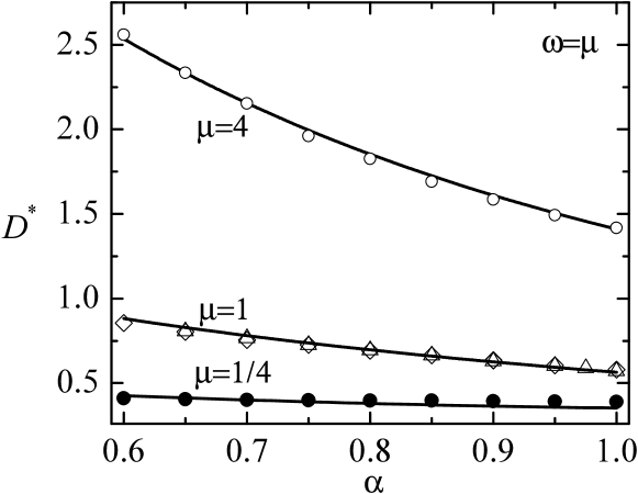
Figure 2: Plot of the reduced diffusion coefficient $D^{*}$ as a function of the (common) coefficient of restitution $\alpha$ for binary mixtures with $\omega=\mu$ in the case of a two-dimensional system ($d=2$). Here, $\omega\equiv\sigma_{1}/\sigma_{2}$ and $\mu\equiv m_{1}/m_{2}$. The symbols are computer simulation results obtained from the mean square displacement and the lines are the theoretical results obtained in the first Sonine approximation. The DSMC results correspond to $\mu=1/4$ ($\bullet$), $\mu=4$ ($\circ$) and $\mu=1$ ($\diamond$). Molecular dynamics results reported in Ref. BRCG00 for $\mu=1$ ($\triangle$) have also been included.

The dependence of $D^{*}$ on the common coefficient of restitution $\alpha_{ij}\equiv\alpha$ is shown in Fig. 2 in the case of hard disks ($d=2$) for three different systems. The symbols refer to DSMC simulations while the lines correspond to the kinetic theory results obtained in the first Sonine approximation GD02 ; GM06 . MD results reported in Ref. BRCG00 when impurities and particles of the gas are mechanically equivalent have also been included. We observe that in the latter case MD and DSMC results are consistent among themselves in the range of values of $\alpha$ explored. This good agreement gives support to the applicability of the inelastic Boltzmann equation beyond the quasielastic limit. It is apparent that the agreement between the first Sonine approximation and simulation results is excellent when impurities and particles of the gas are mechanically equivalent and when impurities are much heavier and/or much larger than the particles of the gas (Brownian limit). However, some discrepancies between simulation an theory are found with decreasing values of the mass ratio $\mu\equiv m_{1}/m_{2}$ and the size ratio $\omega\equiv\sigma_{1}/\sigma_{2}$. These discrepancies are not easily observed in Fig. 2 because of the small magnitude of $D^{*}$ for $\mu=1/4$. For these systems, the second Sonine approximation GM04 improves the qualitative predictions over the first Sonine approximation for the cases in which the gas particles are heavier and/or larger than impurities. This means that the Sonine polynomial expansion exhibits a slow convergence for sufficiently small values of the mass ratio $\mu$ and/or the size ratio $\omega$. This tendency is also present in the case of elastic systems MC84 .

5.2 Shear Viscosity Coefficient of a Heated Gas

The shear viscosity $\eta$ is perhaps the most widely studied transport coefficient in granular fluids. This coefficient can be measured in computer simulations in the special hydrodynamic state of uniform shear flow (USF). At a macroscopic level, this state is characterized by constant partial densities $n_{i}$, uniform temperature $T$, and a linear flow velocity profile $u_{1,k}=u_{2,k}=a_{k\ell}r_{\ell}$, $a_{k\ell}=a\delta_{kx}\delta_{\ell y}$, $a$ being the constant shear rate. In this state, the temperature changes in time due to the competition between two mechanisms: on the one hand, viscous heating and, on the other hand, energy dissipation in collisions. In addition, the mass and heat fluxes vanish by symmetry reasons and the (uniform) pressure tensor is the only nonzero flux of the problem. The relevant balance equation is that for temperature, Eq. (14), which reduces to

$$\partial_{t}T+\frac{2}{dn}aP_{xy}=-(\zeta-\xi)T,$$ (63)

where

$$P_{xy}=\sum_{i=1}^{2}m_{i}\int\;\text{d}{\bf V}V_{x}V_{y}f_{i}({\bf V})$$ (64)

is the $xy$-element of the pressure tensor.

For a granular fluid under USF and in the absence of a thermostatting force ($\xi=0$), the energy balance equation (63) leads to a steady state when the viscous heating effect is exactly balanced by the collisional cooling. This situation will be analyzed in Sec. 10. However, if for instance the mixture is heated by the Gaussian thermostat (29) (with ${\bf v}\to{\bf V}$), then the viscous heating still prevails so that the temperature increases in time. In this case, the collision frequency $\nu_{0}(t)\propto\sqrt{T(t)}$ also grows with $t$ and hence the reduced shear rate $a^{*}(t)=a/\nu_{0}(t)$ (which is the relevant nonequilibrium parameter of the problem) monotonically decreases in time. Under these conditions, the system asymptotically achieves a regime described by linear hydrodynamics and the (reduced) shear viscosity $\eta^{*}=[\nu_{0}(t)/nT(t)]\eta(t)$ can be measured as

$$\eta^{*}=-\lim_{t\to\infty}\frac{P_{xy}^{*}}{a^{*}},$$ (65)

where $P_{xy}^{*}=P_{xy}/nT$. This procedure allows one to identify the shear viscosity of a granular mixture excited by the Gaussian external force (29) and compare it with the predictions given by the Chapman–Enskog method.

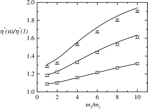
Figure 3: Plot of the ratio $\eta^{*}(\alpha)/\eta^{*}(1)$ as a function of the mass ratio $m_{1}/m_{2}$ for $\sigma_{1}/\sigma_{2}=n_{1}/n_{2}=1$ and three different values of the (common) coefficient of restitution $\alpha$: $\alpha=0.9$ (circles), $\alpha=0.8$ (squares), and $\alpha=0.7$ (triangles). The lines are the theoretical predictions and the symbols refer to the results obtained from the DSMC method.

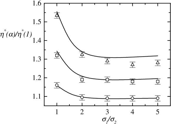
Figure 4: Plot of the ratio $\eta^{*}(\alpha)/\eta^{*}(1)$ as a function of the size ratio $\sigma_{1}/\sigma_{2}$ for $m_{1}/m_{2}=4$, $n_{1}/n_{2}=1$ and three different values of the (common) coefficient of restitution $\alpha$: $\alpha=0.9$ (circles), $\alpha=0.8$ (squares), and $\alpha=0.7$ (triangles). The lines are the theoretical predictions and the symbols refer to the results obtained from the DSMC method.

In Fig. 3, we plot the ratio $\eta^{*}(\alpha)/\eta^{*}(1)$ versus the mass ratio $m_{1}/m_{2}$ in the case of hard spheres ($d=3$) for $\sigma_{1}/\sigma_{2}=1$, $x_{1}=\frac{1}{2}$, and three different values of the (common) coefficient of restitution $\alpha_{ij}\equiv\alpha$. Here, $\eta^{*}(1)$ refers to the elastic value of the shear viscosity coefficient. Again, the symbols represent the simulation data obtained by numerically solving the Boltzmann equation MG03 , while the lines refer to the theoretical results obtained from the Boltzmann equation in the first Sonine approximation. We see that in general the deviation of $\eta^{*}(\alpha)$ from its functional form for elastic collisions is quite important. This tendency becomes more significant as the mass disparity increases. The agreement between the first Sonine approximation and simulation is seen to be in general excellent. This agreement is similar to the one previously found in the monocomponent case BRC99 ; MSG05 ; GM02 . At a quantitative level, the discrepancies between theory and simulation tend to increase as the coefficient of restitution decreases, although these differences are quite small (say, for instance, around 2% at $\alpha=0.7$ in the disparate mass case $m_{1}/m_{2}=10$). The influence of the size ratio on the shear viscosity is shown in Fig. 4 for $m_{1}/m_{2}=4$ and $x_{1}=\frac{1}{2}$ MG03 . We observe again a strong dependence of the shear viscosity on dissipation. However, for a given value of $\alpha$, the influence of $\sigma_{1}/\sigma_{2}$ on $\eta^{*}$ is weaker than the one found before in Fig. 3 for the mass ratio. The agreement for both $\alpha=0.9$ and $\alpha=0.8$ is quite good, except for the largest size ratio at $\alpha=0.8$. These discrepancies become more significant as the dissipation increases, especially for mixtures of particles of very different sizes. In summary, according to the comparison carried out in Figs. 3 and 4, one can conclude that the agreement between theory and simulation extends over a wide range values of the coefficient of restitution, indicating the reliability of the first Sonine approximation for describing granular flows beyond the quasielastic limit.

6 Einstein Relation in Granular Gases

The results presented in Section 5 give some support to the validity of the hydrodynamic description to granular fluids. However, in spite of this support some care is warranted in extending properties of normal fluids to those with inelastic collisions. Thus, for elastic collisions, in the case of an impurity (tracer) particle immersed in a gas the response to an external force on the impurity particle leads to a mobility coefficient proportional to the diffusion coefficient. This is the usual Einstein relation M89 , which is a consequence of the fluctuation-dissipation theorem. A natural question is whether the Einstein relation also applies for granular fluids.

To analyze it, let us consider the tracer limit ($x_{1}\to 0$) and assume that the current of impurities ${\bf j}_{1}^{(1)}$ is only generated by the presence of a weak concentration gradient $\nabla x_{1}$ and/or a weak external field ${\bf F}_{1}$ acting only on the impurity particles. Under these conditions, Eq. (35) becomes

$${\bf j}_{1}^{(1)}=-m_{1}D\nabla x_{1}+\chi_{11}{\bf F}_{1}.$$ (66)

The Einstein ratio $\epsilon^{\prime}$ between the diffusion coefficient $D$ and the mobility coefficient $\chi_{11}$ is defined as

$$\epsilon^{\prime}=m_{1}x_{1}\frac{D}{T\chi_{11}},$$ (67)

where $T\simeq T_{2}$ in the tracer limit. For elastic collisions, the Chapman–Enskog results yield $\epsilon^{\prime}=1$. However, at finite inelasticity the relationship between $D$ and $\chi_{11}$ is no longer simple and, as expected, the Chapman–Enskog expressions for $D$ and $\chi_{11}$ in the case of an unforced granular gas DG01 clearly show that $\epsilon^{\prime}\neq 1$. This means that the Einstein relation does not apply in granular gases. The deviations of the (standard) Einstein ratio $\epsilon^{\prime}$ from unity has three distinct origins: the absence of the Gibbs state (non-Gaussianity of the distribution function of the HCS), time evolution of the granular temperature, and the occurrence of different kinetic temperatures between the impurity and gas particles. The second source of discrepancy can be avoided if the system is driven by an external energy input to achieve a stationary state. With respect to the third reason of violation, this could also be partially eliminated if the temperature of the gas $T$ is replaced by the temperature of the impurity $T_{1}$ in the usual Einstein relation (67). This change yields the modified Einstein ratio

$$\epsilon=m_{1}x_{1}\frac{D}{T_{1}\chi_{11}}.$$ (68)

As a consequence, the only reason for which $\epsilon\neq 1$ is due to the non-Maxwellian behavior of the HCS distribution. Given that the deviations of the gas distribution $f_{2}^{(0)}$ from its Maxwellian form are small GD99 , the discrepancies of $\epsilon$ from unity could be difficult to detect in computer simulations. This conclusion agrees with recent MD simulations BLP04 of granular mixtures subjected to the stochastic driving of the form (30), where no deviations from the (modified) Einstein relation $\epsilon=1$ have been observed for a wide range of values of the coefficients of restitution and parameters of the system.

Figure 5: Plot of the modified Einstein ratio $\epsilon$ versus the coefficient of restitution $\alpha_{12}$ for the Gaussian thermostat in the cases: (a) $\alpha_{22}=\alpha_{12}$, $m_{1}/m_{2}=5$ and $\sigma_{1}/\sigma_{2}=1$; (b) $\alpha_{22}=\alpha_{12}$, $m_{1}/m_{2}=0.5$ and $\sigma_{1}/\sigma_{2}=1$; and (c) $\alpha_{22}=0.5$, $m_{1}/m_{2}=10$ and $\sigma_{1}/\sigma_{2}=1$.

Figure 6: Plot of the Einstein ratio $\epsilon$ versus the coefficient of restitution $\alpha_{12}$ for the stochastic thermostat in the cases: (a) $\alpha_{22}=\alpha_{12}$, $m_{1}/m_{2}=5$ and $\sigma_{1}/\sigma_{2}=1$; (b) $\alpha_{22}=\alpha_{12}$, $m_{1}/m_{2}=0.5$ and $\sigma_{1}/\sigma_{2}=1$; and (c) $\alpha_{22}=0.5$, $m_{1}/m_{2}=10$ and $\sigma_{1}/\sigma_{2}=1$.

To illustrate the influence of dissipation on the Einstein ratio more generally, in Figs. 5 and 6 the Einstein ratio as given by (68) is plotted versus the coefficient of restitution $\alpha_{12}$ for $\sigma_{1}/\sigma_{2}=1$ and different values of the mass ratio $m_{1}/m_{2}$ and the coefficient of restitution $\alpha_{22}$. The results obtained by using the Gaussian thermostat (29) are shown in Fig. 5, while Fig. 6 corresponds to the results derived when the system is heated by the stochastic thermostat (30) G04 . We observe that in general $\epsilon\neq 1$, although its value is very close to unity, especially in the case of the stochastic thermostat, where the deviations from the Einstein relation are smaller than $1\%$. However, in the case of the Gaussian thermostat the deviations from unity are about $8\%$, which could be detected in computer simulations. Figures 5 and 6 also show the fact that the transport properties are affected by the thermostat introduced so that the latter does not play a neutral role in the problem GM02 .

7 Onsager’s Reciprocal Relations in Granular Gases

In the usual language of the linear irreversible thermodynamics for ordinary fluids GM84 , the constitutive equations (35) and (37) for the mass flux and heat flux in the absence of external forces can be written as

$$\mathbf{j}_{i}^{(1)}=-\sum_{j}L_{ij}\left(\frac{\nabla\mu_{j}}{T}\right)_{T}-L_{iq}\frac{\nabla T}{T^{2}}-C_{p}\nabla p,$$ (69)

$$\mathbf{J}_{q}^{(1)}=-L_{qq}\nabla T-\sum_{i}L_{qi}\left(\frac{\nabla\mu_{i}}{T}\right)_{T}-C_{p}^{\prime}\nabla p,$$ (70)

where

$${\bf J}_{q}^{(1)}\equiv{\bf q}^{(1)}-\frac{d+2}{2}T\sum_{i}\frac{{\bf j}_{i}^{(1)}}{m_{i}}$$ (71)

and

$$\left(\frac{\nabla\mu_{i}}{T}\right)_{T}=\frac{1}{m_{i}}\nabla\ln(x_{i}p),$$ (72)

$\mu_{i}$ being the chemical potential per unit mass. In Eqs. (69) and (70), the coefficients $L_{ij}$ are the so-called Onsager phenomenological coefficients and the coefficients $C_{p}$ and $C_{p}^{\prime}$ can be expressed in terms of the transport coefficients associated with the heat and mass fluxes. For elastic fluids, Onsager showed GM84 that time reversal invariance of the underlying microscopic equations of motion implies important constraints on the above set of transport coefficients, namely

$$L_{ij}=L_{ji},\quad L_{iq}=L_{qi},\quad C_{p}=C_{p}^{\prime}=0.$$ (73)

The first two symmetries are called reciprocal relations as they relate transport coefficients for different processes. The last two are statements that the pressure gradient does not appear in any of the fluxes, even though it is admitted by symmetry. Even for a one component fluid, Onsager’s theorem is significant as it leads to a new contribution to the heat flux proportional to the density gradient BDKS98 . Since there is no time reversal symmetry for granular fluids, Eqs. (73) cannot be expected to apply. However, since explicit expressions for all transport coefficients are at hand, the quantitative extent of the violation can be explored.

To make connection with the expressions (35) and (37) for the mass and heat fluxes, respectively, it is first necessary to transform Eqs. (69)–(71) to the variables $x_{1},$ $p,$ $T.$ Since $\nabla x_{1}=-\nabla x_{2}$, Eq. (72) implies

$$\frac{(\nabla\mu_{1})_{T}-(\nabla\mu_{2})_{T}}{T}=\frac{n\rho}{\rho_{1}\rho_{2}}\left[\nabla x_{1}+\frac{n_{1}n_{2}}{n\rho}(m_{2}-m_{1})\nabla\ln p\right].$$ (74)

The coefficients $\{L_{ij},L_{iq},L_{qi},L_{qq},C_{p},C_{p}^{\prime}\}$ then can be easily obtained in terms of the Navier-Stokes transport coefficients introduced in Sec. 4. The result is GMD06

$$L_{11}=-L_{12}=-L_{21}=\frac{m_{1}m_{2}\rho_{1}\rho_{2}}{\rho^{2}}D,\quad L_{1q}=\rho TD^{\prime},$$ (75)

$$L_{q1}=-L_{q2}=\frac{T^{2}\rho_{1}\rho_{2}}{n\rho}D^{\prime\prime}-\frac{d+2}{2}\frac{T\rho_{1}\rho_{2}}{\rho^{2}}(m_{2}-m_{1})D,$$ (76)

$$L_{qq}=\lambda-\frac{d+2}{2}\rho\frac{m_{2}-m_{1}}{m_{1}m_{2}}D^{\prime},$$ (77)

$$C_{p}\equiv\frac{\rho}{p}D_{p}-\frac{\rho_{1}\rho_{2}}{p\rho^{2}}(m_{2}-m_{1})D,$$ (78)

$$C_{p}^{\prime}\equiv L-\frac{d+2}{2}\frac{T}{p}\frac{m_{2}-m_{1}}{m_{1}m_{2}}C_{p}-\frac{n_{1}n_{2}}{np\rho}T^{2}(m_{2}-m_{1})D^{\prime\prime}.$$ (79)

Onsager’s relation $L_{12}=L_{21}$ holds since the diffusion coefficient $D$ is symmetric under the change $1\leftrightarrow 2$ GD02 . However, in general $L_{1q}\neq L_{q1}$, $C_{p}\neq 0$, and $C_{p}^{\prime}\neq 0$ GMD06 . The Chapman-Enskog results GD02 show that there are only two limit cases for which $L_{1q}-L_{q1}=C_{p}=C_{p}^{\prime}=0$: (i) the elastic limit ($\alpha_{ij}=1$) with arbitrary values of masses, sizes and composition and (ii) the case of mechanically equivalent particles with arbitrary values of the (common) coefficient of restitution $\alpha\equiv\alpha_{ij}$. Beyond these limit cases, Onsager’s relations do not apply. At macroscopic level the origin of this failure is due to the cooling of the reference state as well as the occurrence of different kinetic temperatures for both species.

8 Linearized Hydrodynamic Equations and Stability of the Homogeneous Cooling State

As shown in Sec. 4, the Navier-Stokes constitutive equations (35)–(37) have been expressed in terms of a set of experimentally accessible fields such as the composition of species $1$, $x_{1}$, the pressure $p$, the mean flow field ${\bf u}$, and the granular temperature $T$. In terms of these variables and in the absence of external forces, the macroscopic balance equations (12)–(14) become

$$D_{t}x_{1}+\frac{\rho}{n^{2}m_{1}m_{2}}\nabla\cdot\mathbf{j}_{1}=0\;,$$ (80)

$$D_{t}p+p\nabla\cdot\mathbf{u}+\frac{2}{d}\left(\nabla\cdot\mathbf{q}+\mathsf{P}:\nabla\mathbf{u}\right)=-\zeta p,$$ (81)

$$D_{t}\mathbf{u}+\rho^{-1}\nabla\cdot\mathsf{P}=0\;,$$ (82)

$$D_{t}T-\frac{T}{n}\sum_{i}\frac{\nabla\cdot\mathbf{j}_{i}}{m_{i}}+\frac{2}{dn}\left(\nabla\cdot\mathbf{q}+\mathsf{P}:\nabla\mathbf{u}\right)=-\zeta T\;.$$ (83)

When the expressions (35)–(37) for the fluxes and the cooling rate $\zeta\to\zeta^{(0)}$ are substituted into the above exact balance equations (80)–(83) one gets a closed set of hydrodynamic equations for $x_{1},{\bf u},T,$ and $p$. These are the Navier–Stokes hydrodynamic equations for a binary granular mixture:

$$D_{t}x_{1}=\frac{\rho}{n^{2}m_{1}m_{2}}\nabla\cdot\left(\frac{m_{1}m_{2}n}{\rho}D\nabla x_{1}+\frac{\rho}{p}D_{p}\nabla p+\frac{\rho}{T}D^{\prime}\nabla T\right)\;,$$ (84)

$$\left(D_{t}+\zeta\right)p+\frac{d+2}{d}p\nabla\cdot{\bf u} = \frac{2}{d}\nabla\cdot\left(T^{2}D^{\prime\prime}\nabla x_{1}+L\nabla p+\lambda\nabla T\right)$$

$$+\frac{2}{d}\eta\left(\nabla_{\ell}u_{k}+\nabla_{k}u_{\ell}-\frac{2}{d}\delta_{k\ell}\nabla\cdot{\bf u}\right)\nabla_{\ell}u_{k},$$

$$\left(D_{t}+\zeta\right)T+\frac{2}{dn}p\nabla\cdot{\bf u} = -\frac{T}{n}\frac{m_{2}-m_{1}}{m_{1}m_{2}}\nabla\cdot\left(\frac{m_{1}m_{2}n}{\rho}D\nabla x_{1}+\frac{\rho}{p}D_{p}\nabla p\right.$$ (86)

$$\left.+\frac{\rho}{T}D^{\prime}\nabla T\right)+\frac{2}{dn}\nabla\cdot\left(T^{2}D^{\prime\prime}\nabla x_{1}+L\nabla p+\lambda\nabla T\right)$$

$$+\frac{2}{dn}\eta\left(\nabla_{\ell}u_{k}+\nabla_{k}u_{\ell}-\frac{2}{d}\delta_{k\ell}\nabla\cdot\mathbf{u}\right)\nabla_{\ell}u_{k},$$

$$D_{t}u_{\ell}+\rho^{-1}\nabla_{\ell}p=\rho^{-1}\nabla_{k}\eta\left(\nabla_{\ell}u_{k}+\nabla_{k}u_{\ell}-\frac{2}{d}\delta_{k\ell}\nabla\cdot{\bf u}\right)\;.$$ (87)

For the chosen set of fields, $n=p/T$ and $\rho=p\left[\left(m_{1}-m_{2}\right)x_{1}+m_{2}\right]/T$. These equations are exact to second order in the spatial gradients for a low density Boltzmann gas. Note that in Eqs. (84)–(87) the second order contributions to the cooling rate have been neglected. These second order terms have been calculated for a monocomponent fluid BDKS98 and found to be very small relative to corresponding terms from the fluxes. Consequently, they have not been considered in the hydrodynamic equations (84)–(87).

One of the main peculiarities of the granular gases (in contrast to ordinary fluids) is the existence of non-trivial solutions to the Navier–Stokes equations (84)–(87), even for spatially homogeneous states,

$$\partial_{t}x_{1H}=0,\quad\partial_{t}{\bf u}_{H}={\bf 0},$$ (88)

$$\left[\partial_{t}+\zeta\left(x_{1H},T_{H},p_{H}\right)\right]T_{H}=0,\hskip 21.68121pt\left[\partial_{t}+\zeta\left(x_{1H},T_{H},p_{H}\right)\right]p_{H}=0,$$ (89)

where the subscript $H$ denotes the homogeneous state. Since the dependence of the cooling rate $\zeta\left(x_{1H},T_{H},p_{H}\right)$ on $x_{1H},T_{H},p_{H}$ is known GD99 ; GM06 , these first order nonlinear equations can be solved for the time dependence of the homogeneous state. The result is the familiar Haff cooling law for $T(t)$ at constant density H83 ; BP04 :

$$T_{H}(t)=\frac{T_{H}(0)}{\left[1+\zeta(0)t/2\right]^{2}}.$$ (90)

As said before, each partial temperature $T_{i}(t)$ has the same time dependence but with a different value GD99 ,

$$T_{1H}(t)=\frac{\gamma}{1+x_{1}(\gamma-1)}T_{H}(t),\quad T_{2H}(t)=\frac{1}{1+x_{1}(\gamma-1)}T_{H}(t),$$ (91)

where $\gamma=T_{1H}(t)/T_{2H}(t)$ is the time-independent temperature ratio.

Nevertheless, the homogeneous cooling state (HCS) is unstable to sufficiently long wavelength perturbations. For systems large enough to support such spontaneous fluctuations, the HCS becomes inhomogeneous at long times. This feature was first observed in MD simulations of free monocomponent gases GZ93 . In MD simulations the inhomogeneities may grow by the formation of clusters, ultimately aggregating to a single large cluster LH99 ; if cluster growth is suppressed, a vortex field may grow to the system size where periodic boundary conditions can induce a transition to a state with macroscopic shear. The mechanism responsible for the growth of inhomogeneities can be understood at the level of the Navier–Stokes hydrodynamics, where linear stability analysis shows two shear modes and a heat mode to be unstable BDKS98 ; BRC99 ; BP04 ; G05 .

The objective here is to extend this analysis to the case of a binary mixture. To do that, we perform a linear stability analysis of the nonlinear hydrodynamic equations (84)–(87) with respect to this HCS for small initial spatial perturbations. For ordinary fluids such perturbations decay in time according to the hydrodynamic modes of diffusion (shear, thermal, mass) and damped sound propagation HM86 ; RL77 ; BY80 . For inelastic collisions, the analysis is for fixed coefficients of restitution in the long wavelength limit. As will be seen below, the corresponding modes for a granular mixture are then quite different from those for ordinary mixtures. In fact, an alternative study with fixed long wavelength and coefficients of restitution approaching unity yields the usual ordinary fluid modes. Consequently, the nature of the hydrodynamic modes is non uniform with respect to the inelasticity and the wavelength of the perturbation.

Let us assume that the deviations $\delta y_{\alpha}({\bf r},t)=y_{\alpha}({\bf r},t)-y_{H\alpha}(t)$ are small. Here, $\delta y_{\alpha}({\bf r},t)$ denotes the deviation of $\{x_{1},{\bf u},T,p\}$ from their values in the HCS. If the initial spatial perturbation is sufficiently small, then for some initial time interval these deviations will remain small and the hydrodynamic equations (84)–(87) can be linearized with respect to $\delta y_{\alpha}(\mathbf{r},t)$. This leads to a set of partial differential equations with coefficients that are independent of space but which depend on time. As in the monocomponent case BDKS98 ; G05 , this time dependence can be eliminated through a change in the time and space variables, and a scaling of the hydrodynamic fields. We introduce the following dimensionless space and time variables:

$$\tau=\int_{0}^{t}\text{d}t^{\prime}\nu_{0H}(t^{\prime}),\quad{\bf s}=\frac{\nu_{0H}(t)}{v_{0H}(t)}{\bf r},$$ (92)

where $\nu_{0H}(t)$ is an effective collision frequency for hard spheres and $v_{0H}=\sqrt{2T_{H}(m_{1}+m_{2})/m_{1}m_{2}}$. Since $\{x_{1H},{\bf u}_{H},T_{H},p_{H}\}$ are evaluated in the HCS, then Eqs. (88) and (89) hold. A set of Fourier transformed dimensionless variables are then introduced as

$$\rho_{{\bf k}}(\tau)=\frac{\delta x_{1{\bf k}}(\tau)}{x_{1H}},\quad{\bf w}_{{\bf k}}(\tau)=\frac{\delta{\bf u}_{{\bf k}}(\tau)}{v_{0H}(\tau)},\quad\theta_{{\bf k}}(\tau)=\frac{\delta T_{{\bf k}}(\tau)}{T_{H}(\tau)},\quad\Pi_{{\bf k}}(\tau)=\frac{\delta p_{{\bf k}}(\tau)}{p_{H}(\tau)},$$ (93)

where $\delta y_{\alpha{\bf k}}\equiv\{\delta x_{1{\bf k}},\delta{\bf u}_{\bf k},\delta T_{\bf k},\delta p_{\bf k}\}$ is defined as

$$\delta y_{\alpha{\bf k}}(\tau)=\int\text{d}{\bf s}\;e^{-i{\bf k}\cdot{\bf s}}\delta y_{\alpha}({\bf s},\tau).$$ (94)

Note that here the wave vector ${\bf k}$ is dimensionless.

In terms of the above variables, the transverse velocity components ${\bf w}_{\mathbf{k}\perp}={\bf w}_{\bf k}-({\bf w}_{\bf k}\cdot\widehat{{\bf k}})\widehat{{\bf k}}$ (orthogonal to the wave vector ${\bf k}$) decouple from the other four modes and hence can be obtained more easily. They obey the equation

$$\left(\frac{\partial}{\partial\tau}-\frac{\zeta^{*}}{2}+\eta^{*}k^{2}\right){\bf w}_{{\bf k}\perp}={\bf 0},$$ (95)

where $\zeta^{*}=\zeta_{H}/\nu_{0H}$ and

$$\eta^{*}=\frac{\nu_{0H}}{\rho_{H}v_{0H}^{2}}\eta,$$ (96)

where $\rho_{H}=m_{1}n_{1H}+m_{2}n_{2H}$. The solution for ${\bf w}_{{\bf k}\perp}(\tau)$ reads

$${\bf w}_{{\bf k}\perp}(\tau)={\bf w}_{{\bf k}\perp}(0)\exp[s_{\perp}(k)\tau],$$ (97)

where

$$s_{\perp}(k)=\frac{1}{2}\zeta^{*}-\eta^{*}k^{2}.$$ (98)

This identifies $d-1$ shear (transversal) modes. We see from Eq. (98) that there exists a critical wave number $k_{\perp}^{\text{c}}$ given by

$$k_{\perp}^{\text{c}}=\left(\frac{\zeta^{*}}{2\eta^{*}}\right)^{1/2}.$$ (99)

This critical value separates two regimes: shear modes with $k\geq k_{\perp}^{\text{c}}$ always decay while those with $k<k_{\perp}^{\text{c}}$ grow exponentially.

The remaining modes are called longitudinal modes. They correspond to the set $\{\rho_{{\bf k}},\theta_{{\bf k}},\Pi_{{\bf k}},w_{{\bf k}||}\}$ where the longitudinal velocity component (parallel to ${\bf k}$) is $w_{{\bf k}||}={\bf w}_{\bf k}\cdot\widehat{{\bf k}}$. These modes are the solutions of the linear equation GMD06

$$\frac{\partial\delta z_{\alpha{\bf k}}(\tau)}{\partial\tau}=\left(M_{\alpha\beta}^{(0)}+ikM_{\alpha\beta}^{(1)}+k^{2}M_{\alpha\beta}^{(2)}\right)\delta z_{\beta{\bf k}}(\tau),$$ (100)

where $\delta z_{\alpha{\bf k}}(\tau)$ denotes now the four variables $\left\{\rho_{{\bf k}},\theta_{{\bf k}},\Pi_{{\bf k}},w_{{\bf k}||}\right\}$. The matrices in Eq. (100) are given by

$${\sf M}^{(0)}=\left(\begin{array}[]{cccc}0&0&0&0\\ -x_{1}\left(\frac{\partial\zeta^{*}}{\partial x_{1}}\right)_{T,p}&\frac{1}{2}\zeta^{*}&-\zeta^{*}&0\\ -x_{1}\left(\frac{\partial\zeta^{*}}{\partial x_{1}}\right)_{T,p}&\frac{1}{2}\zeta^{*}&-\zeta^{*}&0\\ 0&0&0&\frac{1}{2}\zeta^{*}\end{array}\right),$$ (101)

$${\sf M}^{(1)}=\left(\begin{array}[]{cccc}0&0&0&0\\ 0&0&0&-\frac{2}{d}\\ 0&0&0&-\frac{d+2}{d}\\ 0&0&-\frac{1}{2}\frac{\mu_{12}}{x_{1}\mu+x_{2}}&0\end{array}\right),$$ (102)

$${\sf M}^{(2)}=\left(\begin{array}[]{cccc}-D^{*}&-x_{1}^{-1}D^{\prime*}&-x_{1}^{-1}D_{p}^{*}&0\\ M_{21}^{(2)}&M_{22}^{(2)}&M_{23}^{(2)}&0\\ -\frac{2}{d}x_{1}D^{\prime\prime*}&-\frac{2}{d}\lambda^{*}&-\frac{2}{d}L^{*}&0\\ 0&0&0&-\frac{2}{d}(d-1)\eta^{*}\end{array}\right),$$ (103)

where

$$M_{21}^{(2)}=-x_{1}\left(\frac{2}{d}D^{\prime\prime*}-\frac{1-\mu}{x_{1}\mu+x_{2}}D^{*}\right),$$ (104)

$$M_{22}^{(2)}=\frac{1-\mu}{x_{1}\mu+x_{2}}D^{\prime*}-\frac{2}{d}\lambda^{*},$$ (105)

$$M_{23}^{(2)}=-\frac{2}{d}L^{*}+\frac{1-\mu}{x_{1}\mu+x_{2}}D_{p}^{*}.$$ (106)

In these equations, $\mu=m_{1}/m_{2}$, $x_{i}=n_{iH}/n_{H}$, and we have introduced the reduced Navier–Stokes transport coefficients

$$D^{*}=\frac{\nu_{0H}}{n_{H}v_{0H}^{2}}D,\quad D_{p}^{*}=\frac{\rho_{H}^{2}\nu_{0H}}{m_{1}m_{2}n_{H}^{2}v_{0H}^{2}}D_{p},\quad D^{\prime*}=\frac{\rho_{H}^{2}\nu_{0H}}{m_{1}m_{2}n_{H}^{2}v_{0H}^{2}}D^{\prime},$$ (107)

$$D^{\prime\prime*}=\frac{\nu_{0H}T_{H}}{n_{H}v_{0H}^{2}}D^{\prime\prime},\quad L^{*}=\frac{\nu_{0H}}{v_{0H}^{2}}L,\quad\lambda^{*}=\frac{\nu_{0H}}{n_{H}v_{0H}^{2}}\lambda.$$ (108)

Figure 7: Dispersion relations for $\alpha=0.9$, $x_{1}=0.2$, $\omega=1$ and $\mu=4$.

The longitudinal modes have the form $\exp[s_{n}(k)\tau]$ with $n=1,2,3,4$, where $s_{n}(k)$ are the eigenvalues of the matrix ${\sf M}(k)={\sf M}^{(0)}+ik{\sf M}^{(1)}+k^{2}{\sf M}^{(2)}$, namely, they are the solutions of the quartic equation

$$\det|{\sf M}-s\mathsf{I}|=0.$$ (109)

The solution to (109) for arbitrary values of $k$ is quite intricate. It is instructive to consider first the solutions to these equations in the extreme long wavelength limit, $k=0$. In this case, they are found to be the eigenvalues of the matrix of ${\sf M}^{(0)}$:

$$s_{n}^{(0)}=\left(0,0,-\frac{1}{2}\zeta^{\ast},\frac{1}{2}\zeta^{\ast}\right).$$ (110)

Hence, at asymptotically long wavelengths (${\bf k}=0$) the spectrum of the linearized hydrodynamic equations (both transverse and longitudinal) is comprised of a decaying mode at $-\zeta^{*}/2$, a two-fold degenerate mode at $0$, and a $d$-fold degenerate unstable mode at $\zeta^{*}/2$. Consequently, some of the solutions are unstable. The two zero eigenvalues represent marginal stability solutions, while the negative eigenvalue gives stable solutions. For general initial perturbations all modes are excited. These modes correspond to evolution of the fluid due to uniform perturbations of the HCS, i.e., a global change in the HCS parameters. The unstable modes are seen to arise from the initial perturbations $w_{\mathbf{k}\perp}(0)$ or $w_{\mathbf{k}||}(0)$. The marginal modes correspond to changes in the composition at fixed pressure, density, and velocity, and to changes in $\Pi_{\mathbf{k}}-\theta_{\mathbf{k}}$ at constant composition and velocity. The decaying mode corresponds to changes in the temperature or pressure for $\Pi_{\mathbf{k}}=\theta_{\mathbf{k}}$. The unstable modes may appear trivial since they are due entirely to the normalization of the fluid velocity by the time dependent thermal velocity. However, this normalization is required by the scaling of the entire set of equations to obtain time independent coefficients.

The real parts of the modes $s_{\perp}(k)$ and $s_{n}(k)$ is illustrated in Fig. 7 in the case of hard spheres ($d=3$) for $\alpha\equiv\alpha_{ij}=0.9$, $\sigma_{1}/\sigma_{2}=1$, $x_{1}=0.2$, and $m_{1}/m_{2}=4$. The $k=0$ values correspond to five hydrodynamic modes with two different degeneracies. The shear mode degeneracy remains at finite $k$ but the other is removed at any finite $k$. At sufficiently large $k$ a pair of real modes become equal and become a complex conjugate pair at all larger wave vectors, like a sound mode. The smallest of the unstable modes is that associated with the longitudinal velocity, which couples to the scalar hydrodynamic fields. It becomes negative at a wave vector smaller than that of Eq. (99) and gives the threshold for development of spatial instabilities.

The results obtained here for mixtures show no new surprises relative to the case for a monocomponent gas BDKS98 ; BP04 ; G05 , with only the addition of the stable mass diffusion mode. Of course, the quantitative features can be quite different since there are additional degrees of freedom with the parameter set $\left\{x_{1H},m_{1}/m_{2},\sigma_{1}/\sigma_{2},\alpha_{ij}\right\}$. Also, the manner in which these linear instabilities are enhanced by the nonlinearities may be different from that for the one component case BRC99bis .

9 Segregation in Granular Binary Mixtures: Thermal Diffusion

The analysis of the linearized hydrodynamic equations for a granular binary mixture has shown that the resulting equations exhibit a long wavelength instability for $d$ of the modes. These instabilities lead to the spontaneous formation of velocity vortices and density clusters when the system evolves freely. A phenomenon related with the density clustering is the separation or species segregation. Segregation and mixing of dissimilar grains is perhaps one of the most interesting problems in agitated granular mixtures. In some processes it is a desired and useful effect to separate particles of different types, while in other situations it is undesired and can be difficult to control. A variety of mechanisms have been proposed to describe the separation of particles of two sizes in a mixture of vertically shaken particles. Different mechanisms include void filling, static compressive force, convection, condensation, thermal diffusion, interstitial gas forcing, friction, and buoyancy K04 . However, in spite of the extensive literature published in the past few years on this subject, the problem is not completely understood yet. Among the different competing mechanisms, thermal diffusion becomes one of the most relevant at large shaking amplitude where the sample of macroscopic grains resembles a granular gas. In this regime, binary collisions prevail and kinetic theory can be quite useful to analyze the physical mechanisms involved in segregation processes.

Thermal diffusion is caused by the relative motion of the components of a mixture because of the presence of a temperature gradient. Due to this motion, concentration gradients subsequently appear in the mixture producing diffusion that tends to oppose those gradients. A steady state is finally achieved in which the separation effect arising from thermal diffusion is compensated by the diffusion effect. In these conditions, the so-called thermal diffusion factor $\Lambda_{ij}$ characterizes the amount of segregation parallel to the temperature gradient. In this Section, the thermal diffusion factor is determined from the Chapman–Enskog solution described before.

To make some contact with experiments, let us assume that the binary granular mixture is in the presence of the gravitational field ${\bf g}=-g\hat{{\bf e}}_{z}$, where $g$ is a positive constant and $\hat{{\bf e}}_{z}$ is the unit vector in the positive direction of the $z$ axis. In experiments SUKSS06 , the energy is usually supplied by vibrating horizontal walls so that the system reaches a steady state. Here, instead of considering oscillating boundary conditions, particles are assumed to be heated by the action of the stochastic driving force (30), which mimics a thermal bath. As said above, although the relation between this driven idealized method with the use of locally driven wall forces is not completely understood, it must be remarked that in the case of boundary conditions corresponding to a sawtooth vibration of one wall the condition to determine the temperature ratio coincides with the one derived from the stochastic force DHGD02 . The good agreement between theory and simulation found in Fig. 1 for the temperature ratio confirms this expectation.

The thermal diffusion factor $\Lambda_{ij}$ ($i\neq j$) is defined at the steady state in which the mass fluxes ${\bf j}_{i}$ vanish. Under these conditions, the factor $\Lambda_{ij}$ is given through the relation KCM83

$$-\Lambda_{ij}\nabla\ln T=\frac{1}{x_{i}x_{j}}\nabla x_{i},\quad\Lambda_{ij}+\Lambda_{ji}=0.$$ (111)

The physical meaning of $\Lambda_{ij}$ can be described by considering a granular binary mixture held between plates at different temperatures $T$ (top plate) and $T^{\prime}$ (bottom plate) under gravity. For the sake of concreteness, we will assume that gravity and thermal gradient point in parallel directions, i.e., the bottom is hotter than the top ($T^{\prime}>T$). In addition, without loss of generality, we also assume that $\sigma_{1}>\sigma_{2}$. In the steady state, Eq. (111) describes how the thermal field is related to the composition of the mixture. Assuming that $\Lambda_{12}$ is constant over the relevant ranges of temperature and composition, integration of Eq. (111) yields

$$\ln\frac{x_{1}x_{2}^{\prime}}{x_{2}x_{1}^{\prime}}=\Lambda_{12}\ln\frac{T^{\prime}}{T},$$ (112)

where $x_{i}$ refers to the mole fraction of species $i$ at the top plate and $x_{i}^{\prime}$ refers to the mole fraction of species $i$ at the bottom plate. Consequently, according to Eq. (112), if $\Lambda_{12}>0$, then $x_{1}^{\prime}<x_{1}$, while if $\Lambda_{12}<0$, then $x_{1}^{\prime}>x_{1}$. In summary, when $\Lambda_{12}>0$, the larger particles accumulate at the top of the sample (cold plate), while if $\Lambda_{12}<0$, the larger particles accumulate at the bottom of the sample (hot plate). The former situation is referred to as the Brazil-nut effect (BNE) while the latter is called the reverse Brazil-nut effect (RBNE).

The RBNE was first observed by Hong et al. HQL01 in MD simulations of vertically vibrated systems. They proposed a very simple segregation criterion that was later confirmed by Jenkins and Yoon JY02 by using kinetic theory. More recently, Breu et al. BEKR03 have experimentally investigated conditions under which the large particles sink to the bottom and claim that their experiments confirm the theory of Hong et al. HQL01 provided a number of conditions are chosen carefully. In addition to the vertically vibrated systems, some works have also focused in the last few years on horizontally driven systems showing some similarities to the BNE and its reverse form horizontal . However, it is important to note that the criterion given in Ref. HQL01 is based on some drastic assumptions: elastic particles, homogeneous temperature, and energy equipartition. These conditions preclude a comparison of the kinetic theory derived here with the above simulations.

Figure 8: Phase diagram for BNE/RBNE for mixtures constituted by spheres ($d=3$) of the same mass density and equal total volumes of large and small particles. The data points represent the MD simulation results SUKSS06 for $\alpha=0.78$ when convection is suppressed. Points below (above) the curve correspond to RBNE (BNE).

Some theoretical attempts to assess the influence of non-equipartition on segregation have been recently published. Thus, Trujillo et al. TAH03 have derived an evolution equation for the relative velocity of the intruders starting from the kinetic theory proposed by Jenkins and Yoon JY02 , which applies for weak dissipation. They use constitutive relations for partial pressures that take into account the breakdown of energy equipartition between the two species. However, the influence of temperature gradients, which exist in the vibro-fluidized regime, is neglected in Ref. TAH03 because it is assumed that the pressure and temperature are constant in the absence of the intruder. A more refined theory has recently been provided by Brey et al. BRM05 in the case of a single intruder in a vibrated granular mixture under gravity. The theory displayed in this section covers some of the aspects not accounted for in the previous theories BRM05 ; JY02 ; TAH03 since it is based on a kinetic theory GD02 that goes beyond the quasi-elastic limit JY02 ; TAH03 and applies for arbitrary composition $x_{1}$ (and so, it reduces to the results obtained in Ref. BRM05 when $x_{1}\to 0$). This allows one to assess the influence of composition and dissipation on thermal diffusion in bi-disperse granular gases without any restriction on the parameter space of the system.

To determine the dependence of the coefficient $\Lambda_{12}$ on the parameters of the mixture, we consider a non-convecting (${\bf u}={\bf 0}$) steady state with only gradients along the vertical direction ($z$ axis). In this case, the mass balance equation (12) yields ${\bf j}_{1}={\bf j}_{2}={\bf 0}$, while the momentum equation (13) gives

$$\frac{\partial p}{\partial z}=-\rho g.$$ (113)

To first order in the spatial gradients, the constitutive equation for the mass flux $j_{1,z}$ is given by Eq. (35), i.e.,

$$j_{1,z}=-\frac{m_{1}m_{2}n}{\rho}D\frac{\partial x_{1}}{\partial z}-\frac{\rho}{p}D_{p}\frac{\partial p}{\partial z}-\frac{\rho}{T}D^{\prime}\frac{\partial T}{\partial z},$$ (114)

where the susceptibility coefficient $\chi_{ij}=0$ in the particular case of the gravitational force. The condition $j_{1,z}=0$ yields

$$\frac{\partial x_{1}}{\partial z}=\frac{\rho^{3}}{m_{1}m_{2}np}\frac{D_{p}}{D}g-\frac{\rho^{2}}{m_{1}m_{2}p}\frac{D^{\prime}}{D}\frac{\partial T}{\partial z},$$ (115)

where use has been made of Eq. (113). Substitution of Eq. (115) into Eq. (111) leads to

$$\Lambda_{12}=\frac{n\rho^{2}}{\rho_{1}\rho_{2}}\frac{D^{\prime}-D_{p}g^{*}}{D},$$ (116)

where

$$g^{*}\equiv\frac{\rho g}{n\left(\partial T/\partial z\right)}<0$$ (117)

is the reduced gravity acceleration. Since the mutual diffusion coefficient $D$ is positive GD02 ; GM06 , the sign of $\Lambda_{12}$ is determined by the sign of the quantity $D^{\prime}-D_{p}g^{*}$. This result is general since it goes beyond the regime of density considered.

Figure 9: Phase diagram for BNE/RBNE in three dimensions for $\alpha_{ij}=0.7$ and three values of composition: (a) $x_{1}=0$, (b) $x_{1}=0.3$, and (c) $x_{1}=0.7$. Points below (above) each curve correspond to RBNE (BNE).

Figure 10: Phase diagram for BNE/RBNE in three dimensions for $x_{1}=\frac{1}{2}$ and three values of the (common) coefficient of restitution: (a) $\alpha=0.9$, (b) $\alpha=0.8$, and (c) $\alpha=0.5$. Points below (above) each curve correspond to RBNE (BNE).

To gain some insight into the explicit dependence of $D^{\prime}$ and $D_{p}$ on the parameter space of the system, one has to resort to a kinetic theory description. For a low-density gas, the expressions of the coefficients $D^{\prime}$ and $D_{p}$ in the first-Sonine approximation are given by

$$D^{\prime}=0,\quad D_{p}=\frac{\rho_{1}p}{\rho^{2}\nu}\frac{x_{2}}{x_{2}+x_{1}\gamma}\left(\frac{\gamma}{\mu}-1\right),$$ (118)

where $\nu$ is the (positive) collision frequency GM06

$$\nu=\frac{2\pi^{(d-1)/2}}{d\Gamma\left(\frac{d}{2}\right)}n\sigma_{12}^{d-1}v_{0}(1+\alpha_{12})\left(\frac{\theta_{1}+\theta_{2}}{\theta_{1}\theta_{2}}\right)^{1/2}\left(x_{2}\mu_{21}+x_{1}\mu_{12}\right).$$ (119)

Given that the driving stochastic term does not play a neutral role in the transport, it must be remarked that the expressions for the transport coefficients obtained in the driven case slightly differ from the ones derived in the free cooling case GD02 ; GM06 .

Consequently, according to Eqs. (116) and (118), the sign of $\Lambda_{12}$ is the same as that of the pressure diffusion coefficient $D_{p}$. The condition $\Lambda_{12}=0$ (or equivalently, $D_{p}=0$) provides the criterion for the transition from BNE to RBNE. Equation (118) shows that the sign of $D_{p}$ is determined by the value of the control parameter

$$\theta\equiv\frac{\gamma}{\mu}=\frac{m_{2}T_{1}}{m_{1}T_{2}}.$$ (120)

This parameter gives the mean square velocity of the large particles relative to that of the small particles. Thus, when $\theta>1$ ($\theta<1$), the thermal diffusion factor is positive (negative), which leads to BNE (RBNE). The criterion for the transition condition from BNE to RBNE is $\theta=1$, i.e.,

$$\frac{m_{1}}{m_{2}}=\frac{T_{1}}{T_{2}}.$$ (121)

In the case of equal granular temperatures (energy equipartition), $\theta\to\mu^{-1}$ and so segregation is predicted for particles that differ in mass, no matter what their diameters may be JY02 . It must be remarked that, due to the lack of energy equipartition, the condition $\theta=1$ is rather complicated since it involves all the parameter space of the system. In particular, even when the species differ only by their respective coefficients of restitution they also segregate when subject to a temperature gradient. This is a novel pure effect of inelasticity on segregation G06 ; SGNT06 . On the other hand, the criterion (121) for the transition BNE$\Longleftrightarrow$RBNE is the same as the one found previously in Ref. TAH03 when $\alpha_{ij}$ is close to 1 and in Ref. BRM05 in the intruder limit case ($x_{1}\to 0$). However, as said before, the results obtained here are more general since they cover all the range of the parameter space of the system.

To illustrate size segregation driven by thermal diffusion, we consider mixtures constituted by spheres ($d=3$) of the same material and equal total volumes of large and small particles. In this case, $m_{1}/m_{2}=(\sigma_{1}/\sigma_{2})^{3}$ and $x_{2}/x_{1}=(\sigma_{1}/\sigma_{2})^{3}$. Figure 8 shows the phase diagram BNE/RBNE for this kind of systems. The data points represent the simulation results obtained by Schröter et al. SUKSS06 for $\alpha=0.78$ in agitated mixtures constituted by particles of the same density. To the best of my knowledge, this is one of the few experiments in which thermal diffusion has been isolated from the remaining segregation mechanisms K04 . Our results show that, for a given value of the coefficient of restitution, the RBNE is dominant at small diameter ratios. However, since non-equipartition grows with increasing diameter ratio, the system shows a crossover to BNE at sufficiently large diameter ratios. This behavior agrees qualitatively well with the results reported in Ref. SUKSS06 at large shaking amplitudes, where thermal diffusion becomes the relevant segregation mechanism. At a quantitative level, we observe that the results are also consistent with the simulation results reported in SUKSS06 when periodic boundary conditions are used to suppress convection since they do not observe a change back to BNE for diameter ratios up to 3 (see red squares in Fig. 11 of SUKSS06 ). Although the parameter range explored in MD simulations is smaller than the one analyzed here, one is tempted to extrapolate the simulation data presented in Ref. SUKSS06 to roughly predict the transition value of the diameter ratio at $\alpha=0.78$ (which is the value of the coefficient of restitution considered in the simulations). Thus, if one extrapolates from the simulation data at the diameter ratios of $\sigma_{1}/\sigma_{2}=2$ and $\sigma_{1}/\sigma_{2}=3$, one sees that the transition from RBNE to BNE might be around $\sigma_{1}/\sigma_{2}=10$, which would quantitatively agree with the results reported in Fig. 8. Figure 8 also shows that the BNE is completely destroyed in the quasielastic limit ($\alpha\simeq 1$).

Let us now investigate the influence of composition on segregation. Figure 9 shows a typical phase diagram in the three-dimensional case for $\alpha_{ij}\equiv\alpha=0.7$ and three different values of the mole fraction $x_{1}$. The lines separate the regimes between BNE and RBNE. We observe that the composition of the mixture has significant effects in reducing the BNE as the concentration of larger particles increases. In addition, for a given value of composition, the transition from BNE to RBNE may occur following two paths: (i) along the constant mass ratio $m_{2}/m_{1}$ with increasing size ratio $\sigma_{1}/\sigma_{2}$, and (ii) along the constant size ratio with increasing mass ratio $m_{2}/m_{1}$. The influence of dissipation on the phase diagrams BNE/RBNE is illustrated in Fig. 10 for $d=3$ in the case of an equimolar mixture ($x_{1}=\frac{1}{2}$) and three values of the (common) coefficient of restitution $\alpha$. We observe that the role played by inelasticity is quite important since the regime of RBNE increases significantly with dissipation. Similar results are found for other values of composition.

In summary, thermal diffusion (which is the relevant segregation mechanism in agitated granular mixtures at large shaking amplitudes) can been analyzed by the Boltzmann kinetic theory. This theory is able to explain some of the experimental and/or MD segregation results SUKSS06 observed within the range of parameter space explored. A more quantitative comparison in the dilute regime with MD simulations is needed to show the relevance of the Boltzmann equation to analyze segregation driven by a thermal gradient. As said before, comparison with MD simulations in the tracer limit case ($x_{1}\to 0$) BRM05 for a dilute gas has shown the reliability of the inelastic Boltzmann equation to describe segregation. In this context, one expects that the same agreement observed before in the intruder case BRM05 is maintained when $x_{1}$ is different from zero.

10 Steady States: Uniform Shear Flow

In the preceding sections, the Navier–Stokes equations (constitutive equations that are linear in the hydrodynamic gradients) have been shown to be quite useful to describe appropriately several problems in granular mixtures. However, under some circumstances large gradients occur and more complex constitutive equations are required. The need for more complex constitutive equations does not signal a breakdown of hydrodynamics TG98 , only a failure of the Navier–Stokes approximation DB99 . Although in this case the Chapman-Enskog method can be carried out to second order in gradients (Burnett order), it is likely that failure of the Navier-Stokes description signals the need for other methods to construct the normal solution that are not based on a small gradient expansion.

One of the most interesting problems in granular fluids is the simple or uniform shear flow (USF) G03 ; C90 . As described in Sec. 5, this state is characterized by uniform density and temperature and a simple shear with the local velocity field given by $u_{1,x}=u_{2,x}=ay,u_{y}=u_{z}=0$, where $a$ is the constant shear rate. The USF is a well-known nonequilibrium problem widely studied, for both granular C90 ; USF ; WA99 ; AL02 ; CH02 and conventional GS03 ; Ha83 gases. However, the nature of this state is quite different in both systems since a steady state is achieved for granular fluids when viscous (shear) heating is compensated for by energy dissipation in collisions:

$$aP_{xy}=-\frac{d}{2}nT\zeta.$$ (122)

This steady state is what we want to analyze in this section. The balance equation (122) shows the intrinsic connection between the shear field and dissipation in the system. This contrasts with the description of USF for elastic fluids where a steady state is not possible unless an external thermostat is introduced GS03 . Note that the hydrodynamic steady shear flow state associated with the condition (122) is inherently beyond the scope of the Navier–Stokes or Newtonian hydrodynamic equations SGD04 . The reason for this is the existence of an internal mechanism, collisional cooling, that sets the strength of the velocity gradient in the steady state. For normal fluids, this scale is set by external sources (boundary conditions, driving forces) that can be controlled to admit the conditions required for Navier–Stokes hydrodynamics. In contrast, collisional cooling is fixed by the mechanical properties of the particles making up the fluid. This observation is significant because it prevents the possibility of measuring the Newtonian shear viscosity for granular fluids in the steady USF AL02 ; CH02 . More generally, it provides a caution regarding the simulation of other steady states to study Navier–Stokes hydrodynamics when the gradients are strongly correlated to the collisional cooling SGD04 .

From a microscopic point of view, the simple shear flow problem becomes spatially uniform in the local Lagrangian frame moving with the flow velocity ${\bf u}$. In this frame GS03 ; LE72 ; DSBR86 , the velocity distribution functions adopt the form: $f_{i}({\bf r},{\bf v})\to f_{i}({\bf V})$, where $V_{k}=v_{k}-a_{k\ell}r_{\ell}$ is the peculiar velocity. Here, $a_{k\ell}=a\delta_{kx}\delta_{\ell y}$. Under these conditions, the set of Boltzmann kinetic equations (with ${\cal F}_{i}=0$) for an isolated system reads

$$-aV_{y}\frac{\partial}{\partial V_{x}}f_{i}({\bf V})=\sum_{j=1}^{2}\;J_{ij}[{\bf V}|f_{i},f_{j}]\;,\quad(i=1,2).$$ (123)

The most relevant transport properties in a shear flow problem are obtained from the pressure tensor ${\sf P}={\sf P}_{1}+{\sf P}_{2}$, where ${\sf P}_{i}$ is the partial pressure tensor of the species $i$ given by

$$P_{i,k\ell}=m_{i}\int\;\text{d}{\bf V}V_{k}V_{\ell}f_{i}({\bf V}).$$ (124)

The trace of ${\sf P}_{i}$ defines the partial temperatures $T_{i}$ as $T_{i}=\text{Tr}{\sf P}_{i}/dn_{i}$. As said before, these temperatures measure the mean kinetic energy of each species. The elements of the pressure tensor ${\sf P}_{i}$ can be obtained by multiplying the Boltzmann equation (123) by $m_{i}{\bf V}{\bf V}$ and integrating over ${\bf V}$. The result is

$$a_{km}P_{i,m\ell}+a_{\ell m}{P}_{i,mk}=\sum_{j=1}^{2}{A}_{ij,k\ell},$$ (125)

where we have introduced the collisional moments ${\sf A}_{ij}$ as

$$A_{ij,k\ell}=m_{i}\int\text{d}{\bf V}V_{k}V_{\ell}J_{ij}[{\bf V}|f_{i},f_{j}].$$ (126)

From Eq. (125), in particular, one gets the balance equation for the partial temperature $T_{i}$

$$aP_{i,xy}=-\frac{d}{2}p_{i}\zeta_{i},$$ (127)

where $p_{i}=n_{i}T_{i}$ is the partial pressure of species $i$ and $\zeta_{i}$ is defined by Eq. (10). According to Eq. (127), the (steady) partial temperature in the simple shear flow problem can be obtained by equating the viscous heating term $a|P_{i,xy}|$ to the collisional cooling term $(d/2)p_{i}\zeta_{i}$.

The determination of ${\sf A}_{ij}$ requires the knowledge of the velocity distribution functions $f_{i}$. This is quite a formidable task, even in the monocomponent case USF . However, as in the elastic case, one expects to get a good estimate of ${\sf A}_{ij}$ by using Grad’s approximation FK72 :

$$f(\mathbf{V})\to f_{i,M}(\mathbf{V})\left(1+\frac{m_{i}}{2T_{i}}C_{i,k\ell}V_{k}V_{\ell}\right),$$ (128)

where $f_{i,M}$ is a Maxwellian distribution at the temperature of the species $i$, i.e.,

$$f_{i,M}({\bf V})=n_{i}\left(\frac{m_{i}}{2\pi T_{i}}\right)^{d/2}\exp\left(-\frac{m_{i}V^{2}}{2T_{i}}\right).$$ (129)

As happens in the case of homogeneous states, in general the three temperatures $T$, $T_{1}$, and $T_{2}$ are different in the inelastic case. For this reason we choose the parameters in the Maxwellians so that it is normalized to $n_{i}$ and provides the exact second moment of $f_{i}$. The Maxwellians $f_{i,M}$ for the two species can be quite different due to the temperature differences. This aspect is essential in a two-temperature theory and has not been taken into account in most of the previous studies JM89 ; WA99 ; AL02 . The coefficient ${\sf C}_{i}$ can be identified by requiring the moments with respect to ${\bf V}{\bf V}$ of the trial function (128) to be the same as those for the exact distribution $f_{i}$. This leads to

$${\sf C}_{i}=\frac{{\sf P}_{i}}{p_{i}}-\mathsf{I}$$ (130)

With this approximation, the Boltzmann collisional moments ${\sf A}_{ij}$ can be explicitly evaluated. The result is MG02 ; G02

$${\sf A}_{ij} = -\frac{2\pi^{(d-1)/2}}{d\Gamma(d/2)}m_{i}n_{i}n_{j}\mu_{ji}\sigma_{ij}^{d-1}\left(\frac{2T_{i}}{m_{i}}+\frac{2T_{j}}{m_{j}}\right)^{3/2}(1+\alpha_{ij})$$ (131)

$$\times\left\{\mu_{ji}\left[\frac{T_{j}-T_{i}}{(m_{j}/m_{i})T_{i}+T_{j}}+\frac{1-\alpha_{ij}}{2}\right]\mathsf{I}+\frac{1}{1+(m_{i}T_{j}/m_{j}T_{i})}\right.$$

$$\left.\times\left[\frac{{\sf C}_{i}-{\sf C}_{j}}{1+(m_{j}T_{i}/m_{i}T_{j})}+\frac{d+3}{2(d+2)}\lambda_{ij}\left({\sf C}_{i}+\frac{m_{i}T_{j}}{m_{j}T_{i}}{\sf C}_{j}\right)\right]\right\},$$

where

$$\lambda_{ij}=2\mu_{ji}\frac{T_{j}-T_{i}}{(m_{j}/m_{i})T_{i}+T_{j}}+\frac{\mu_{ji}}{d+3}(2d+3-3\alpha_{ij}).$$ (132)

The partial cooling rates $\zeta_{i}$ can be easily obtained from Eqs. (10) and (131).

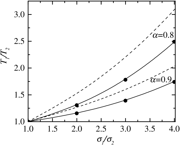
Figure 11: Plot of the temperature ratio $T_{1}/T_{2}$ as a function of the size ratio $\sigma_{1}/\sigma_{2}=(m_{1}/m_{2})^{1/2}$ for a two-dimensional system in the case $x_{1}=1/2$ and two different values of the (common) coefficient of restitution: $\alpha=0.9$ and $\alpha=0.8$. The solid lines are the theoretical predictions based on Grad’s solution, while the symbols refer to the DSMC results. The dashed lines correspond to the results obtained from the stochastic thermostat condition (31).

Substitution of Eq. (131) into the set of equations (125) allows one to get the partial pressure tensor ${\sf P}_{i}$ in terms of the temperature ratio $\gamma=T_{1}/T_{2}$ and the parameters of the mixture. The temperature ratio can be obtained from Eq. (127) as

$$\gamma=\frac{x_{2}\zeta_{2}P_{1,xy}}{x_{1}\zeta_{1}P_{2,xy}}.$$ (133)

When the expressions of ${\sf P}_{i}$ and $\zeta_{i}$ are used in Eq. (133), one gets a closed equation for the temperature ratio $\gamma$, that can be solved numerically. In Fig. 11 we plot $\gamma$ versus the diameter ratio $\sigma_{1}/\sigma_{2}$ for a two-dimensional ($d=2$) granular gas with $x_{1}=1/2$ and two different values of $\alpha$. The symbols refer to the simulation data obtained from the DSMC method GM03a . Here, we have assumed that the disks are made of the same material, and hence $\alpha_{ij}=\alpha$ and $m_{1}/m_{2}=(\sigma_{1}/\sigma_{2})^{2}$. The dependence of $\gamma$ on $\sigma_{1}/\sigma_{2}$ obtained in the homogeneous steady state driven by the stochastic thermostat (30) is also included for comparison. It is clearly seen that the kinetic theory results based on Grad’s solution agree very well with simulation data, even for quite large values of the size ratio. In addition, the thermostat results overestimate the simulation ones (especially for large mass ratio), showing that the properties of the system are not insensitive to the way at which the granular gas is driven.

Figure 12: Plot of the reduced pressure $p^{*}$ versus the mass ratio $\mu=m_{1}/m_{2}$ for a two-dimensional system with $\sigma_{1}=\sigma_{2}$, $x_{1}=1/2$ and $\alpha=0.9$. The solid line corresponds to the theoretical predictions derived from Grad’s solution, the dotted line refers to the latter theory but using the expression of $T_{1}/T_{2}$ obtained from the stochastic thermostat condition (31), and the dashed line is the result obtained from Grad’s solution by assuming the equality of the partial temperatures ($\gamma=1$). The symbols are the DSMC results.

Figure 13: Plot of the reduced shear viscosity $\eta^{*}$ versus the mass ratio $\mu=m_{1}/m_{2}$ for a two-dimensional system with $\sigma_{1}=\sigma_{2}$, $x_{1}=1/2$ and $\alpha=0.9$. The solid line corresponds to the theoretical predictions derived from Grad’s solution, the dotted line refers to the latter theory but using the expression of $T_{1}/T_{2}$ obtained from the stochastic thermostat condition (31), and the dashed line is the result obtained from Grad’s solution by assuming the equality of the partial temperatures ($\gamma=1$). The symbols are the DSMC results.

Let us now consider the transport coefficients. To analyze the rheological properties in the steady state, it is convenient to introduce dimensionless quantities. As usual AL02 , for a low-density gas we introduce the reduced pressure $p^{*}$ and the reduced shear viscosity $\eta^{*}$ as

$$p^{*}=\frac{p\nu^{2}}{\rho_{1}v_{0}^{2}a^{2}},$$ (134)

$$\eta^{*}=\frac{\eta\nu^{2}}{\rho_{1}v_{0}^{2}a},$$ (135)

where $\eta=-P_{xy}/a$ is the non-Newtonian shear viscosity, $P_{xy}=P_{1,xy}+P_{2,xy}$ and $\nu=[\pi^{(d-1)/2}/\Gamma(d/2)]n\sigma_{12}^{d-1}v_{0}$. In Figs. 12 and 13, we plot $p^{*}$ and $\eta^{*}$, respectively, as functions of the mass ratio $\mu=m_{1}/m_{2}$ for an equal-size ($\sigma_{1}=\sigma_{2}$) binary mixture of disks ($d=2$) with $x_{1}=1/2$ and $\alpha=0.9$. We have also included the predictions for $p^{*}$ and $\eta^{*}$ given by the kinetic theory but taking the expression of $\gamma$ derived when the system is driven by the stochastic thermostat BT02 . We observe again in both figures an excellent agreement between the Boltzmann theory based on Grad’s solution and the DSMC results, even for very disparate values of the mass ratio. With respect to the influence of energy nonequipartition, Fig. 12 shows that $p^{*}$ presents a non-monotonic behaviour with the mass ratio whereas the theoretical predictions with the equipartition assumption monotonically increase with $\mu$. In the case of the shear viscosity, as seen in Fig. 13, both theories (with and without energy nonequipartition) predict a non-monotonic dependence of $\eta^{*}$ on $\mu$. However, at a quantitative level, the influence of energy nonequipartition is quite significant over the whole range of mass ratios considered. The non-monotonic dependence of $p^{*}$ and $\eta^{*}$ on $\mu$ obtained here from the Boltzmann kinetic theory also agrees qualitatively well with MD simulations carried out for bidisperse dense systems AL02 . Thus, for instance, the minimum values of $p^{*}$ and $\eta^{*}$ are located close to $\mu=10$ in both dilute and dense cases. Moreover, the predictions for the transport properties given from the present theory by taking the stochastic thermostat expression of $\gamma$ are quite close to those obtained from the actual value of $\gamma$, especially for large mass ratios.

11 Summary and Concluding Remarks

The primary objective of this review has been to derive the Navier–Stokes hydrodynamic equations of a binary mixture of granular gases from the (inelastic) Boltzmann kinetic theory. The Chapman–Enskog method CC70 ; FK72 is used to solve the Boltzmann equation up to the first order in the spatial gradients and the associated transport coefficients are given in terms of the solutions of a set of linear integral equations. These equations have been approximately solved by taking the leading terms in a Sonine polynomial expansion. Comparison with controlled numerical simulations in some idealized conditions shows quite a good agreement between theory and simulation even for strong dissipation. This supports the idea that the hydrodynamic description (derived from kinetic theory) appears to be a powerful tool for analysis and predictions of rapid flow gas dynamics of polydisperse systems D02 .

The reference state in the Chapman–Enskog expansion has been taken to be an exact solution of the uniform Boltzmann equation. An interesting and important result of this solution GD99 is that the partial temperatures (which measure the mean kinetic energy of each species) are different. This does not mean that there are additional degrees of freedom since the partial temperatures can be expressed in terms of the global temperature. This is confirmed by noting that Haff’s cooling law H83 (in the free cooling case) is the hydrodynamic mode at long wavelengths and MD simulations confirm that the global temperature dominates after a transient period of a few collision times DHGD02 . In this case, only the global temperature should appear among the hydrodynamic fields. Nevertheless, the species temperatures play a new and interesting secondary role GMD06 . For an ordinary (molecular) gas, there is a rapid velocity relaxation in each fluid cell to a local equilibrium state on the time scale of a few collisions (e.g., as illustrated by the approach to Haff’s law). Subsequently, the equilibration among cells occurs via the hydrodynamic equations. In each cell the species velocity distributions are characterized by the species temperatures. These are approximately the same due to equipartition, and the hydrodynamic relaxation occurs for the single common temperature FK72 . A similar rapid velocity relaxation occurs for granular gases in each small cell, but to a universal state different from local equilibrium and one for which equipartition no longer occurs. Hence, the species temperatures $T_{i}$ are different from each other and from the overall temperature $T$ of the cell. Nevertheless, the time dependence of all temperatures (in the free cooling case) is the same in this and subsequent states, i.e., they are proportional to the global temperature. This implies that the species temperatures do not provide any new dynamical degree of freedom at the hydrodynamic stage. However, they still characterize the shape of the partial velocity distributions and affect the quantitative averages calculated with these distributions. The transport coefficients for granular mixtures therefore have new quantitative effects arising from the time independent temperature ratios for each species GD02 . This view contrasts with some recent works recent , where additional equations for each species temperature have been included among the hydrodynamic set. However, as mentioned before, this is an unnecessary complication, describing additional kinetics beyond hydrodynamics that is relevant only on the time scale of a few collisions.

Another important issue discussed here has been the applicability of the Navier–Stokes transport coefficients since their expressions are not restricted to weak inelasticity D02 . However, the Navier–Stokes hydrodynamic equations themselves may or may not be limited with respect to inelasticity, depending on the particular states studied. The Chapman–Enskog method assumes that the relative changes of the hydrodynamic fields over distances of the order of the mean free path are small. In the case of ordinary fluids this can be controlled by the initial or boundary conditions. For granular gases the situation is more complicated since in some cases (e.g., steady states such as the simple shear flow problem SGD04 ) the boundary conditions imply a relationship between dissipation and gradients so that both cannot be chosen independently. In these cases, the Navier–Stokes approximation only holds for nearly elastic particles. However, the transport coefficients characterizing the Navier–Stokes hydrodynamic equations are nonlinear functions of the coefficients of restitution, regardless the applicability of those equations.

In spite of the above cautions, the Navier–Stokes approximation is appropriate and accurate for a wide class of flows. One group refers to spatial perturbations of the homogeneous cooling state (HCS) for an isolated system. Both MD and DSMC simulations BRC99 have confirmed the dependence of the Navier–Stokes transport coefficients on the coefficient of restitution, and application of the Navier–Stokes hydrodynamics with these coefficients to describe cluster formation has also been confirmed quantitatively BRC99bis . The same kinetic theory results apply to driven systems as well. This is so since the reference state is a local HCS whose parameters vary throughout the system to match the physical values in each cell. Examples include application of Navier–Stokes hydrodynamics from kinetic theory to symmetry breaking and density/temperature profiles in vertical vibrated gases, for comparison with simulation Brey . Similar comparison with Navier–Stokes hydrodynamics of the latter and of supersonic flow past a wedge in real experiments has been given Caldera ; Swinney , showing both qualitative and quantitative agreement. In summary, the Navier–Stokes equations with the constitutive equations presented here remain an important and useful description for a wide class of granular flow, although more limited than for normal gases.

The explicit knowledge of the transport coefficients and the cooling rate allows one to make some applications of the Navier–Stokes hydrodynamic equations. One of them has been to obtain the linear hydrodynamic equations for small perturbations of the homogenous cooling state. The resulting equations exhibit a long wavelength instability for three of the modes. This is quite similar to the case of a monocomponent granular gas BDKS98 ; BP04 ; G05 , and in fact the same modes are unstable here. The additional diffusion mode for two species behaves as for a normal fluid.

On the other hand, the constitutive equations for the mass and heat fluxes of a granular binary mixture differ from those obtained for ordinary fluids CC70 . This is because the usual restrictions of irreversible thermodynamics no longer apply. These restrictions include Onsager’s reciprocal relations among various transport coefficients and the extent to which these are violated has also been shown here. Another application of the Navier–Stokes equations has been to assess the violation of the Einstein relation between the diffusion and mobility coefficients. In the undriven case, the analysis shows that this violation is due to three independent reasons DG01 : the absence of the Gibbs state, the cooling of the reference state, and the occurrence of different temperatures for the particle and surrounding fluid. However, when the mixture is subjected to stochastic driving, a modified Einstein relation suggested by recent MD simulations BLP04 has also been analyzed. In this case, the results show that the deviations of the (modified) Einstein ratio from unity are in general very small (less than $1\%$), in agreement with MD simulations BLP04 .

Thermal diffusion becomes the relevant segregation mechanism in agitated granular mixtures at large shaking amplitudes. In these conditions, the use of the Boltzmann kinetic theory for low-density gases appears justified to understand the influence of thermal gradient on segregation phenomena. The thermal diffusion factor in a heated granular mixture has been explicitly evaluated from the Chapman–Enskog solution to the Boltzmann equation. The results show that the criterion for the transition Brazil-nut effect $\Longleftrightarrow$reverse Brazil-nut effect is provided by the control parameter $\theta=m_{2}T_{1}/m_{1}T_{2}$ G06 ; BRM05 ; TAH03 . Given that the energy equipartition is broken, the condition $\theta=1$ is quite complex since it involves all the parameters of the system: composition, masses, sizes, and coefficients of restitution. The Boltzmann kinetic theory results agree qualitatively well with recent MD simulations SUKSS06 within the range of parameter space analyzed.

The hydrodynamic description also seems to be justified in the case of steady states that are inherently beyond the scope of the Navier–Stokes hydrodynamic equations. The reason for this non-Newtonian behavior is the existence of an internal mechanism, collisional cooling, that sets the scale of the spatial gradients in the steady state. For ordinary fluids, this scale can be externally controlled by external sources so that the conditions for Navier–Stokes hydrodynamics apply. On the other hand, for granular gases, collisional cooling is fixed by the mechanical properties of the particles of the system and so the gas can depart from the Navier–Stokes description. One well-known example of steady states is the simple or uniform shear flow (USF). However, in spite of the extensive prior work on USF for granular fluids USF ; AL02 ; CH02 , the inherent non-Newtonian character of this state has not been conveniently taken into account. In fact, MD simulations of steady USF have been used for granular fluids to measure the Newtonian or Navier–Stokes shear viscosity. The results derived here from Grad’s solution and DSMC simulations show that USF is an ideal testing ground for the study of rheology since any choice of the shear rate and the coefficients of restitution $\alpha_{ij}$ will provide non-Newtonian effects. It is one of the fascinating features of granular fluids that phenomena associated with complex fluids are more easily accessible than for simple atomic fluids D02 ; G01 .

Hydrodynamics derived from hard-sphere models have found widespread use in the description of numerous industrial processes involving solid particles. Of particular relevance are high-speed, gas-solid flows as found in pneumatic conveyors (of ores, chemicals, grains, etc.) and fluidized beds (for fluid catalytic cracking, power generation, granulation of pharmaceutical powders, synthesis of fine chemicals like titania, etc.). Such descriptions are now standard features of commercial and research codes. Those codes rely upon accurate transport properties and a first order objective is to assure this accuracy from a careful theoretical treatment. As shown in this review, the price of this approach, in contrast to more phenomenological approaches, is an increasing complexity of the expressions as the systems become more complex.

The analysis carried out in this presentation has been focused on mixtures in the dilute regime, where the collisional transfer contributions to the transport coefficients are neglected and only their kinetic contributions are considered. A further step is to develop a theory for moderately dense granular mixtures. This will provide a fundamental basis for the application of hydrodynamics under realistic conditions. Possible extension of the present Boltzmann kinetic theory to higher densities can be done in the context of the Enskog kinetic equation FK72 . Preliminary results GM03 have been restricted to the uniform shear flow state to get directly the shear viscosity coefficient of a heated granular mixture. The extension of this study GM03 to states with gradients of concentration, pressure, and temperature is somewhat intricate due to subtleties associated with the spatial dependence of the pair correlations functions considered in the revised Enskog theory. A future work is to extend the results derived for moderately dense mixtures of smooth elastic hard spheres MCK83 to inelastic collisions. This would allow us to assess the influence of density on the different problems addressed in this review. Of course, the precise expressions for transport coefficients in this case will be even more complex than for a dilute gas due to the expanded parameter space. However, this complexity is not a problem for implementation in a code.

As shown along this overview, granular mixtures exhibit a wide range of interesting phenomena for which the Navier–Stokes hydrodynamic equations can be considered as an accurate and practical tool. However, due to their complexity, many of their features are not fully understood. Kinetic theory and hydrodynamics (in the broader sense) can be expected to provide some insight into the understanding of such complex materials.

Acknowledgments

I want to acknowledge J. W. Dufty, J. M. Montanero, and A. Santos in their roles as collaborators and critics for much of the material discussed here. Partial support of the Ministerio de Ciencia y Tecnología (Spain) through Grant No. FIS2004-01399 (partially financed by FEDER funds) and from the European Community’s Human Potential Programme HPRN-CT-2002-00307 (DYGLAGEMEM) is also acknowledged.

References

- (1) P. K. Haff, J. Fluid Mech. 134, 187 (1983).
- (2) L. P. Kadanoff, Rev. Mod. Phys. 71, 435 (1999).
- (3) See for instance, J.-P. Hansen and I. R. McDonald, Theory of Simple Liquids (Academic Press, London, 1986).
- (4) S. Chapman and T. G. Cowling, The Mathematical Theory of Nonuniform Gases (Cambridge University Press, Cambridge, 1970).
- (5) J. J. Brey, J. W. Dufty, C. S. Kim, and A. Santos, Phys. Rev. E 58, 4638 (1998).
- (6) J. J. Brey and D. Cubero, in Granular Gases, edited by T. Pöschel and S. Luding (Lectures Notes in Physics, Springer, Vol. 564, 2001), pp. 59–78.
- (7) J. J. Brey, M. J. Ruiz-Montero, and D. Cubero, Europhys. Lett. 48, 359 (1999).
- (8) J. J. Brey, M. J. Ruiz-Montero, D. Cubero, and R. García-Rojo, Phys. Fluids 12, 876 (2000).
- (9) J. J. Brey and M. J. Ruiz-Montero, Phys. Rev. E 70, 051301 (2004).
- (10) J. M. Montanero, A. Santos, and V. Garzó, in Rarefied Gas Dynamics 24, edited by M. Capitelli (American Institute of Physics, Vol. 762, 2005), pp. 797–802; preprint cond-mat/0411219.
- (11) J. W. Dufty, J. Phys.: Condens. Matt. 12, A47 (2000).
- (12) J. W. Dufty, in Recent Research Develop. in Stat. Phys. 2, 21 (2002) and preprint cond-mat/0108444.
- (13) I. Goldhirsch, Annu. Rev. Fluid Mech. 35, 267 (2003).
- (14) J. T. Jenkins and F. Mancini, Phys. Fluids A 1, 2050 (1989); P. Zamankhan, Phys. Rev. E 52, 4877 (1995); B. Arnarson and J. T. Willits, Phys. Fluids 10, 1324 (1998); J. T. Willits and B. Arnarson, ibid. 11, 3116 (1999); M. Alam, J. T. Willits, B. Arnarson, and S. Luding, ibid. 14, 4085 (2002); B. Arnarson and J. T. Jenkins, ibid. 16, 4543 (2004); D. Serero, I. Goldhirsch, S. H. Noskowicz, and M.-L. Tan, J. Fluid Mech. 554, 237 (2006).
- (15) V. Garzó and J. W. Dufty, Phys. Rev. E 60, 5706 (1999).
- (16) See for instance, J. M. Montanero and V. Garzó, Gran. Matt. 4, 17 (2002); A. Barrat and E. Trizac, ibid. 4, 57 (2002); S. R. Dahl, C. M. Hrenya, V. Garzó, and J. W. Dufty, Phys. Rev. E 66, 041301 (2002); R. Pagnani, U. M. B. Marconi, and A. Puglisi, Gran. Matt. 66, 051304 (2002); D. Paolotti, C. Cattuto, U. M. B. Marconi, and A. Puglisi, ibid. 5, 75 (2003); P. Krouskop and J. Talbot, Phys. Rev. E 68, 021304 (2003); H. Wang, G. Jin, and Y. Ma, ibid. 68, 031301 (2003); J. J. Brey, M. J. Ruiz-Montero, and F. Moreno, Phys. Rev. Lett. 95, 098001 (2005); Phys. Rev. E 73, 031301 (2006); M. Schröter, S. Ulrich, J. Kreft, J. B. Swift, and H. L. Swinney, Phys. Rev. E 74, 011307 (2006).
- (17) R. D. Wildman and D. J. Parker, Phys. Rev. Lett. 88, 064301 (2002); K. Feitosa and N. Menon, ibid. 88, 198301 (2002); M. Schröter, S. Ulrich, J. Kreft, J. B. Swift, and H. L. Swinney, Phys. Rev. E 74, 011307 (2006).
- (18) J. Jenkins and F. Mancini, J. Appl. Mech. 54, 27 (1987).
- (19) V. Garzó and J. W. Dufty, Phys. Fluids 14, 1476 (2002).
- (20) V. Garzó, J. M. Montanero, and J. W. Dufty, Phys. Fluids 18, 083305 (2006).
- (21) J. M. Montanero and V. Garzó, Phys. Rev. E 67, 021308 (2003).
- (22) V. Garzó and J. M. Montanero, Phys. Rev. E 69, 021301 (2004).
- (23) J. W. Dufty and V. Garzó, J. Stat. Phys. 105, 723 (2001).
- (24) V. Garzó, Physica A 343, 105 (2004).
- (25) V. Garzó, Europhys. Lett. 75, 521 (2006).
- (26) C. S. Campbell, Annu. Rev. Fluid Mech. 22, 57 (1990).
- (27) In the case of a monocomponent system, see for instance, C. K. K. Lun, S. B. Savage, D. J. Jeffrey, and N. Chepurniy, J. Fluid Mech. 140, 223 (1984); J. T. Jenkins and M. W. Richman, ibid. 192, 313 (1988); C. S. Campbell, ibid. 203, 449 (1989); M. A. Hopkins and H. H. Shen, ibid. 244, 477 (1992); P. J. Schmid and H. K. Kytömaa, ibid. 264, 255 (1994); C. K. K. Lun and A. A. Bent, ibid. 258, 335 (1994); I. Goldhirsch and M. L. Tan, Phys. Fluids 8, 1752 (1996); N. Sela, I. Goldhirsch, and S. H. Noskowicz, ibid. 8, 2337 (1997); J. J. Brey, M. J. Ruiz-Montero, and F. Moreno, Phys. Rev. E 55, 2846 (1997); C.-S. Chou and M. W. Richman, Physica A 259, 430 (1998); C.-S. Chou ibid. 287, 127 (2000); 290, 341 (2001); J. M. Montanero, V. Garzó, A. Santos, and J. J. Brey, J. Fluid Mech. 389, 391 (1999); A. Astillero and A. Santos, Phys. Rev. E 72, 031309 (2005).
- (28) V. Garzó and A. Santos, Kinetic Theory of Gases in Shear Flows. Nonlinear Transport (Kluwer Academic, Dordrecht, 2003).
- (29) A. Santos, V. Garzó, and J. W. Dufty, Phys. Rev. E 69, 061303 (2004).
- (30) A. Goldshtein and M. Shapiro, J. Fluid Mech. 282, 75 (1995).
- (31) J. J. Brey, J. W. Dufty, and A. Santos, J. Stat. Phys. 87, 1051 (1997).
- (32) T. P. C. van Noije and M. H. Ernst, Gran. Matt. 1, 57 (1998).
- (33) J. M. Montanero and V. Garzó, Gran. Matt. 4, 17 (2002).
- (34) S. R. Dahl, C. M. Hrenya, V. Garzó, and J. W. Dufty, Phys. Rev. E 66, 041301 (2002).
- (35) D. J. Evans and G. P. Morriss, Statistical Mechanics of Nonequilibrium Liquids (Academic Press, London, 1990).
- (36) W. G. Hoover, Computational Statistical Mechanics (Elsevier, Amsterdam, 1991).
- (37) J. M. Montanero and A. Santos, Gran. Matt. 2, 53 (2000).
- (38) D. R. M. Williams and F. C. McKintosh, Phys. Rev. E 54, R9 (1996).
- (39) C. Henrique, G. Batrouni, and D. Bideau, Phys. Rev. E 63, 011304 (2000).
- (40) A. Barrat and E. Trizac, Gran. Matt. 4, 52 (2002).
- (41) M. Schröter, S. Ulrich, J. Kreft, J. B. Swift, and H. L. Swinney, Phys. Rev. E 74, 011307 (2006).
- (42) J. J. Brey, M. J. Ruiz-Montero, and F. Moreno, Phys. Rev. Lett. 95, 098001 (2005); Phys. Rev. E 73, 031301 (2006).
- (43) J. Ferziger and H. Kaper, Mathematical Theory of Transport Processes in Gases (North-Holland, Amsterdam, 1972).
- (44) V. Garzó and J. M. Montanero, preprint cond-mat/0604552.
- (45) V. Garzó and J.W. Dufty, Phys. Rev. E 59, 5895 (1999).
- (46) J. F. Lutsko, Phys. Rev. E 72, 021306 (2005).
- (47) G. A. Bird, Molecular Gas Dynamics and the Direct Simulation Monte Carlo of Gas Flows (Clarendon, Oxford, 1994).
- (48) J. A. McLennan, Introduction to Nonequilibrium Statistical Mechanics (Prentice-Hall, New Jersey, 1989).
- (49) A. Santos and J. W. Dufty, Phys. Rev. Lett. 97, 058001 (2006).
- (50) M. López de Haro and E. G. D. Cohen, J. Chem. Phys. 80, 408 (1984).
- (51) V. Garzó and J. M. Montanero, Physica A 313, 336 (2002).
- (52) A. Barrat, V. Loreto, and A. Puglisi, Physica A 334, 513 (2004).
- (53) S. R. de Groot and P. Mazur, Nonequilibrium Thermodynamics (Dover, New York, 1984).
- (54) N. Brilliantov and T. Pöschel, Kinetic Theory of Granular Gases (Oxford University Press, Oxford, 2004).
- (55) I. Goldhirsch and G. Zanetti, Phys. Rev. Lett. 70, 1619 (1993); I. Goldhirsch, M.L. Tan, and G. Zanetti, J. Sci. Comput. 8, 1 (1993).
- (56) S. Luding and H.J. Herrmann, Chaos 9, 673 (1999).
- (57) V. Garzó, Phys. Rev. E 72, 021106 (2005).
- (58) P. Résibois and M. de Leener, Classical Kinetic Theory of Fluids (John Wiley, NY, 1977).
- (59) J. P. Boon and S. Yip, Molecular Hydrodynamics (Dover, NY, 1980).
- (60) J. J. Brey, M. J. Ruiz-Montero, and D. Cubero, Phys. Rev. E 60, 3150 (1999).
- (61) See, for instance, A. Kudrolli, Rep. Prog. Phys. 67, 209 (2004).
- (62) J. M. Kincaid, E. G. D. Cohen, and M. López de Haro, J. Chem. Phys. 86, 963 (1983).
- (63) D. C. Hong, P. V. Quinn, and S. Luding, Phys. Rev. Lett. 86, 3423 (2001).
- (64) J. T. Jenkins and D. K. Yoon, Phys. Rev. Lett. 88, 194301 (2002); D. K. Yoon and J. T. Jenkins, Phys. Fluids 18, 073303 (2006).
- (65) A. P. J. Breu, H. M. Ensner, C. A. Kruelle, and I. Rehberg, Phys. Rev. Lett. 90, 014302 (2003).
- (66) T. Schautz, R. Brito, C. A. Kruelle, and I. Rehberg, Phys. Rev. Lett. 95, 028001 (2005) and references therein.
- (67) L. Trujillo, M. Alam, and H. J. Herrmann, Europhys. Lett. 64, 190 (2003).
- (68) D. Serero, I. Goldhirsch, S. H. Noskowicz, and M.-L. Tan, J. Fluid Mech. 554, 237 (2006).
- (69) M. L. Tan and I. Goldhirsch, Phys. Rev. Lett. 81, 3022 (1998).
- (70) J. W. Dufty and J. J. Brey, Phys. Rev. Lett. 82, 4566 (1999).
- (71) J. T. Willits and B. Arnarson, Phys. Fluids 11, 3116 (1999); M. Alam, J. Willits, B. Arnarson, and S. Luding, ibid. 14, 4085 (2002).
- (72) M. Alam and S. Luding, Gran. Matt. 4, 139 (2002); J. Fluid Mech. 476, 69 (2003); Phys. Fluids 17, 063303 (2005).
- (73) M. Alam and C. M. Hrenya, Phys. Rev. E 63, 0613018 (2001); R. Clelland and C. M. Hrenya, ibid. 65, 031301 (2002); S. R. Dahl, R. Clelland, and C. M. Hrenya, Phys. Fluids 14, 1972 (2002); S. R. Dahl, R. Clelland, and C. M. Hrenya, Powder Tech., 138, 7 (2003); S. R. Dahl and C. M. Hrenya, Phys. Fluids 16, 1 (2004); H. Iddir, H. Arastoopour, and C. M. Hrenya, Powder Tech. 151, 117 (2005).
- (74) See for instance, Nonlinear Fluid Behavior, edited by H. J. M. Hanley (North-Holland, Amsterdam, 1983).
- (75) A. W. Lees and S. F. Edwards, J. Phys. C 5, 1921 (1972).
- (76) J. W. Dufty, A. Santos, J. J. Brey, and R. F. Rodríguez, Phys. Rev. A 33, 459 (1986).
- (77) J. M. Montanero and V. Garzó, Physica A 310, 17 (2002).
- (78) V. Garzó, Phys. Rev. E 66, 021308 (2002).
- (79) V. Garzó and J. M. Montanero, Gran. Matt. 5, 165 (2003).
- (80) L. Huilin, D. Gidaspow, and E. Manger, Phys. Rev. E 64, 061301 (2001); M.F. Ramahan, J. Naser, and P. J. Witt, Powder Tech. 138, 82 (2003); J. E. Galvin, S. R. Dahl, and C. M. Hrenya, J. Fluid Mech. 528, 207 (2005).
- (81) J. J. Brey, M. J. Ruiz-Montero, F. Moreno, and R. García-Rojo, Phys. Rev. E 63, 061305 (2001); ibid. 65, 061302 (2002)
- (82) X. Yang, C. Huan, D. Candela, R. W. Mair, and R. L. Walsworth, Phys. Rev. Lett. 88, 044301 (2002); C. Huan, X. Yang, D. Candela, R. W. Mair, and R. L. Walsworth, Phys. Rev. E 69, 041302 (2004).
- (83) C. Bizon, M. D. Shattuck, J. B. Swift, and Harry L. Swinney, Phys. Rev. E 60, 4340 (1999); E. C. Rericha, C. Bizon, M. D. Shattuck, and H. L. Swinney, Phys. Rev. Lett. 88, 014302 (2002).
- (84) I. Goldhirsch, in Granular Gases, edited by T. Pöschel and S. Luding (Lectures Notes in Physics, Springer, Vol. 564, 2001), pp. 79–99.
- (85) V. Garzó and J. M. Montanero, Phys. Rev. E 68, 041302 (2003).
- (86) M. López de Haro, E. G. D. Cohen, and J. M. Kincaid, J. Chem. Phys. 78, 2746 (1983).