Spin-polarized transport through weakly coupled double quantum dots in the Coulomb-blockade regime

Abstract

We analyze cotunneling transport through two quantum dots in series weakly coupled to external ferromagnetic leads. In the Coulomb blockade regime the electric current flows due to third-order tunneling, while the second-order single-barrier processes have indirect impact on the current by changing the occupation probabilities of the double dot system. We predict a zero-bias maximum in the differential conductance, whose magnitude is conditioned by the value of the inter-dot Coulomb interaction. This maximum is present in both magnetic configurations of the system and results from asymmetry in cotunneling through different virtual states. Furthermore, we show that tunnel magnetoresistance exhibits a distinctively different behavior depending on temperature, being rather independent of the value of inter-dot correlation. Moreover, we find negative TMR in some range of the bias voltage.

I Introduction

Transport properties of double quantum dots (DQDs) have recently attracted much interest. ono02 ; derWielRMP03 ; hazalzetPRB01 ; golovachPRB04 ; graberPRB06 ; cotaPRL05 ; mcclurePRL07 ; liuPRB05 ; wunschPRB06 ; franssonPRB06 ; franssonNT06 ; inarrea06 ; datta07 This is because these structures are ideal systems to study the fundamental interactions between electrons and spins. wolf01 ; loss02 ; maekawa02 ; zutic04 ; maekawa06 Double quantum dots exhibit a variety of interesting effects, such as for example current rectification due to the Pauli spin blockade, ono02 ; franssonPRB06 ; franssonNT06 ; inarrea06 ; datta07 negative differential conductance, liuPRB05 formation of molecular states, graberPRB06 spin pumping, hazalzetPRB01 ; cotaPRL05 etc. Furthermore, double quantum dots are also being considered for future applications in quantum computing. lossPRA98 Experimentally, such systems may be realized for example in lateral and vertical semiconductor quantum dots. ono02 ; mcclurePRL07 ; liuPRB05 ; johnsonPRB05 Another implementation of DQDs are single wall metallic carbon nanotubes with top gate electrodes, which enable changing of charge on each dot separately, as well as the intrinsic DQD parameters. graberPRB06 ; jorgensenAPL06 ; sapmazNL06 ; graber06

The goal of this paper is to analyze transport properties of DQDs weakly coupled to ferromagnetic leads in the Coulomb blockade regime. When the leads are ferromagnetic, transport strongly depends on the magnetic configuration of the system, giving rise to tunnel magnetoresistance (TMR), spin accumulation, exchange field, etc. julliere75 ; barnas98 ; takahashi98 ; bulka00 ; rudzinski01 ; koenigPRL03 ; braunPRB04 ; weymannPRB05 ; weymannPRB07 In the Coulomb blockade regime the electric current flows due to higher-order tunneling processes (cotunneling), while the first-order tunneling processes (sequential tunneling) are exponentially suppressed. weymannPRB05 ; nazarov ; kang ; averin92 The problem of spin-polarized cotunneling has been so far addressed mainly in the case of single quantum dots. weymannPRB05 ; weymannPRB07 ; weymannPRBBR05 ; braigPRB05 ; weymannEPJ05 ; weymannPRB06 ; weymannEPL06 ; souza06 For example, it was shown that tunnel magnetoresistance exhibits distinctively different behavior depending on the number of electrons on the dot. weymannPRB05 Moreover, the zero-bias anomaly was found in the differential conductance when magnetic moments of the leads form antiparallel configuration. weymannPRBBR05 Another interesting behavior was predicted for quantum dots coupled to ferromagnetic leads with non-collinear alignment of magnetizations – the exchange field was found to increase the differential conductance for certain non-collinear configurations, as compared to the parallel one. weymannPRB07 ; franssonEPL05 On the other hand, it was shown experimentally for nonmagnetic systems that the conductance of quantum dots in the cotunneling regime may serve as a handle to determine the spectroscopic g-factor. kogan04

In the case of double quantum dots considered in this paper, in the Coulomb blockade regime the electric current flows due to third-order tunneling processes, while the single-barrier second-order processes together with third-order processes determine the double dot occupation probabilities. Assuming that double quantum dot is occupied by two electrons in equilibrium, one on each dot, we calculate the differential conductance $G$ and tunnel magnetoresistance TMR. We show that differential conductance exhibits a maximum at the zero bias. We further distinguish two different mechanisms leading to this new zero-bias anomaly. The first one is an asymmetry in cotunneling through different virtual states of the DQD system, which leads to an enhancement of $G$ at zero bias. Such asymmetry is induced by a finite value of the inter-dot Coulomb interaction. This mechanism is rather independent of magnetic configuration of the system. The second mechanism leading to the zero-bias maximum in differential conductance is the interplay between spin accumulation and third-order tunneling processes carrying the current. This mechanism does depend on the magnetic configuration of the system and, as we show in the sequel, is found to be more efficient in the antiparallel configuration. We also analyze the behavior of TMR and show that the TMR exhibits a maximum at zero bias, which strongly depends on the temperature. Furthermore, the TMR may become negative in some range of the bias voltage.

Finally, we note that there are several experimental realizations of single quantum dots attached to ferromagnetic leads, chye02 ; ralph02 ; heersche06 ; zhang05 ; tsukagoshi99 ; zhao02 ; jensen05 ; sahoo05 ; pasupathy04 ; fertAPL06 ; hamaya06 while experimental data on spin-polarized transport through double quantum dots is lacking. We believe that the results presented in this paper will be of assistance in discussing future experiments.

II Model and method

The schematic of a double quantum dot coupled to ferromagnetic leads is shown in Fig. 1. It is assumed that the magnetizations of the leads are oriented collinearly, so that the system can be either in the parallel or antiparallel magnetic configuration. The Hamiltonian $\hat{H}$ of the DQD system is given by, $\hat{H}=\hat{H}_{\rm L}+\hat{H}_{\rm R}+\hat{H}_{\rm DQD}+\hat{H}_{\rm T}$. The first two terms describe noninteracting itinerant electrons in the leads, $\hat{H}_{j}=\sum_{{\mathbf{k}}\sigma}\varepsilon_{j{\mathbf{k}}\sigma}c^{\dagger}_{j{\mathbf{k}}\sigma}c_{j{\mathbf{k}}\sigma}$ for the left ($j={\rm L}$) and right ($j={\rm R}$) lead, where $\varepsilon_{j{\mathbf{k}}\sigma}$ is the energy of an electron with the wave vector ${\mathbf{k}}$ and spin $\sigma$ in the lead $j$, and $c^{\dagger}_{j{\mathbf{k}}\sigma}$ ($c_{j{\mathbf{k}}\sigma}$) denotes the respective creation (annihilation) operator. The double dot is described by the Hamiltonian

$$\hat{H}_{\rm DQD} = \sum_{j={\rm L,R}}\sum_{\sigma}\varepsilon_{j}n_{j\sigma}+\sum_{j={\rm L,R}}U_{j}n_{j\uparrow}n_{j\downarrow}$$ (1)

$$+ U^{\prime}\sum_{\sigma\sigma^{\prime}}n_{\rm L\sigma}n_{\rm R\sigma^{\prime}}\,,$$

with $n_{j\sigma}=d^{\dagger}_{j\sigma}d_{j\sigma}$, where $d^{\dagger}_{j\sigma}$ ($d_{j\sigma}$) is the creation (annihilation) operator of an electron with spin $\sigma$ in the left ($j={\rm L}$) or right ($j={\rm R}$) quantum dot, and $\varepsilon_{j}$ is the corresponding single-particle energy. The Coulomb interaction on the left (right) dot is described by $U_{\rm L}$ ($U_{\rm R}$). The last part of $\hat{H}_{\rm DQD}$ corresponds to the inter-dot Coulomb correlation, whose strength is given by $U^{\prime}$. As we are interested in the low bias voltage regime where the system is in the Coulomb blockade, it is justifiable to assume that the energy level of each dot is independent of the bias voltage. For the sake of clarity of further discussion we also assume $\varepsilon_{\rm L}=\varepsilon_{\rm R}\equiv\varepsilon$ and $U_{\rm L}=U_{\rm R}\equiv U$.

We note that in a general case, the exchange interaction between spins in the two dots may lead to the formation of singlet and triplet states. graberPRB06 However, this exchange interaction was found to be rather small as compared to the other energy scales, ono02 and thus, following previous theoretical works, wunschPRB06 ; aghassi06 we will neglect it.

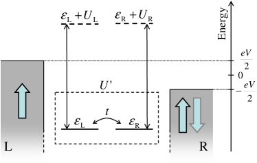
Figure 1: (color online) Schematic of a double quantum dot coupled to ferromagnetic leads. The magnetic moments of the leads can form either parallel or antiparallel configuration. The system is symmetrically biased.

Tunneling processes between the two dots and electrodes are described by the Hamiltonian,

$$\hat{H}_{\rm T}=\sum_{j={\rm L,R}}\sum_{{\mathbf{k}}\sigma}\left(t_{j}c^{\dagger}_{j{\mathbf{k}}\sigma}d_{j\sigma}+h.c.\right)+\left(td^{\dagger}_{\rm L\sigma}d_{\rm R\sigma}+h.c.\right)\,,$$ (2)

where $t_{j}$ denotes the tunnel matrix elements between the $j$th lead and the $j$th dot, and $t$ describes the hopping between the two quantum dots. Coupling of the $j$th dot to the $j$th lead can be expressed as $\Gamma_{j}^{\sigma}=2\pi|t_{j}|^{2}\rho_{j}^{\sigma}$, with $\rho_{j}^{\sigma}$ being the spin-dependent density of states of the corresponding lead. With the definition of the spin polarization of lead $j$, $p_{j}=(\rho_{j}^{+}-\rho_{j}^{-})/(\rho_{j}^{+}+\rho_{j}^{-})$, the coupling can be expressed as, $\Gamma_{j}^{+(-)}=\Gamma_{j}(1\pm p_{j})$, with $\Gamma_{j}=(\Gamma_{j}^{+}+\Gamma_{j}^{-})/2$. Here, $\Gamma_{j}^{+}$ and $\Gamma_{j}^{-}$ describe the coupling of the $j$th dot to the spin-majority and spin-minority electron bands of lead $j$, respectively. As reported in Ref. kogan04, , typical values of the coupling strength are of the order of tens of $\mu$eV. In the following, we assume symmetric couplings, $\Gamma_{\rm L}=\Gamma_{\rm R}\equiv\Gamma/2$, and equal spin polarizations of the leads, $p_{\rm L}=p_{\rm R}\equiv p$.

In this paper we analyze spin-dependent transport through double quantum dot in the case of the Coulomb blockade regime. We assume that in equilibrium each dot is singly occupied, so that there are two electrons in the DQD system. This transport regime can be realized for example in lateral quantum dots mcclurePRL07 ; liuPRB05 ; johnsonPRB05 or in single wall carbon nanotubes with top gate electrodes. graberPRB06 ; jorgensenAPL06 ; sapmazNL06 ; graber06 In such devices by changing the respective gate voltages one can tune the charge on each dot separately and also change the strength of the coupling $t$ between the two dots. Furthermore, we also note that in DQDs the on-level interaction $U$ is usually larger than the inter-dot interaction $U^{\prime}$. In the case where the DQD is doubly occupied and $U>U^{\prime}$, the system can be in four different states $|\chi\rangle$, namely $|\uparrow\uparrow\rangle=|\uparrow\rangle|\uparrow\rangle$, $|\uparrow\downarrow\rangle=|\uparrow\rangle|\downarrow\rangle$, $|\downarrow\uparrow\rangle=|\downarrow\rangle|\uparrow\rangle$, $|\downarrow\downarrow\rangle=|\downarrow\rangle|\downarrow\rangle$, where the first (second) ket corresponds to the left (right) dot. The occupation of the other two-particle states $|\rm d0\rangle=|\uparrow\downarrow\rangle|0\rangle$ and $|0\rm d\rangle=|0\rangle|\uparrow\downarrow\rangle$ is suppressed due to large on-level interaction on the dots.

In the Coulomb blockade the charge fluctuations are suppressed and the system is in a well-defined charge state. As a consequence, all tunneling processes leading to a change of the DQD charge state are exponentially suppressed. The current can thus flow due to higher-order tunneling processes (cotunneling) through virtual states in the double quantum dot. weymannPRB05 ; nazarov ; kang ; averin92 The lowest-order processes which give a dominant contribution to electric current flowing through the DQD structure in the case of Coulomb blockade are the third-order tunneling processes. Generally, the rate for an $n$th-order ($n\geq 2$) tunneling from lead $j$ to lead $j^{\prime}$ associated with a change of the double dot state from $\chi$ into $\chi^{\prime}$ is given by averin92

$${\gamma^{(n)}}_{\rm jj^{\prime}}^{\chi\rightarrow\chi^{\prime}}=\frac{2\pi}{\hbar}\left|\sum_{v_{1},v_{2},\dots,v_{n-1}}\frac{\langle\Phi_{j^{\prime}}^{\chi^{\prime}}|H_{\rm T}|\Phi_{v_{1}}\rangle\langle\Phi_{v_{1}}|H_{\rm T}|\Phi_{v_{2}}\rangle\times\dots\times\langle\Phi_{v_{n-1}}|H_{\rm T}|\Phi_{j}^{\chi}\rangle}{(\varepsilon_{i}-\varepsilon_{v_{1}})(\varepsilon_{i}-\varepsilon_{v_{2}})\times\dots\times(\varepsilon_{i}-\varepsilon_{v_{n-1}})}\right|^{2}\delta(\varepsilon_{i}-\varepsilon_{f})\,,$$ (3)

where $\varepsilon_{i}$ and $\varepsilon_{f}$ denote the energies of initial and final states and $|\Phi_{j}^{\chi}\rangle$ is the state of the system with an electron in the lead $j$ and the double dot in state $|\chi\rangle$, while $|\Phi_{v_{n}}\rangle$ denotes a virtual state of the DQD system and $\varepsilon_{v_{n}}$ its energy. From the above expression one can determine the third-order ($n=3$) tunneling rates that give the main contribution to electric current. We note that there are also tunneling events that do not affect the DQD charge state but can have an influence on transport. These are the second-order processes which take place through a single tunnel barrier, either left or right. Such single-barrier processes contribute to the electric current in an indirect way, namely by changing the occupation probabilities and this way the current. The rate of single-barrier second-order cotunneling is given by Eq. (3) for $n=2$ and $j=j^{\prime}$. It is also worth noting that among different higher-order tunneling events one can distinguish the elastic (non-spin-flip) and inelastic (spin-flip) processes. The former ones change the state of the double dot $(\chi\neq\chi^{\prime})$, while the latter ones do not $(\chi=\chi^{\prime})$.

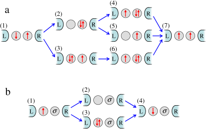
Figure 2: (color online) Examples of possible tunneling processes through double quantum dot in the Coulomb blockade regime. The third-order process (a) from left to right lead, where $|\uparrow\downarrow\rangle$ is the initial state (1) and $|\uparrow\uparrow\rangle$ is the final state (7), takes place via five virtual states (2)-(6). This process contributes directly to the current flowing through the system. The second-order process through the left barrier (b), with $|\uparrow\sigma\rangle$ ($|\downarrow\sigma\rangle$) being the initial (1) [finite (4)] state, where $\sigma=\uparrow,\downarrow$, affects the occupations of the double quantum dot. This process takes place via two virtual states (2)-(3).

Examples of possible processes in the case of the Coulomb blockade regime are shown in Fig. 2. The upper part of the figure presents a third-order process from the left to right lead which contributes to electric current. This is an inelastic process which leads to a change of the double dot state from $|\downarrow\uparrow\rangle$ to $|\uparrow\uparrow\rangle$. It takes place through five virtual states, as sketched in Fig. 2a. On the other hand, the bottom part of Fig. 2 displays a single-barrier second-order process, occurring via two virtual states. This process does not contribute to electric current but affects the DQD occupation probabilities. The process shown in Fig. 2b takes place through the left barrier and changes the double dot state from $|\uparrow\sigma\rangle$ into $|\downarrow\sigma\rangle$, with $\sigma=\uparrow,\downarrow$. To make the discussion more transparent, in Appendix we present the explicit formulas for the rates corresponding to the two processes shown in Fig. 2.

By calculating all the second-order single-barrier and third-order rates one can determine the occupation probabilities from the following stationary master equation

$$0 = \sum_{jj^{\prime}}\sum_{\chi^{\prime}}\left[-\left({\gamma^{(2)}}_{jj}^{\chi\rightarrow\chi^{\prime}}+{\gamma^{(3)}}_{jj^{\prime}}^{\chi\rightarrow\chi^{\prime}}\right)P_{\chi}\right.$$ (4)

$$+ \left.\left({\gamma^{(2)}}_{jj}^{\chi^{\prime}\rightarrow\chi}+{\gamma^{(3)}}_{jj^{\prime}}^{\chi^{\prime}\rightarrow\chi}\right)P_{\chi^{\prime}}\right]\,,$$

where $P_{\chi}$ denotes the probability for the double dot to be in state $|\chi\rangle$. The occupations are fully determined with the aid of the normalization condition, $\sum_{\chi}P_{\chi}=1$. The third-order current flowing through the system from the left to right lead is then given by

$$I=e\sum_{\chi\chi^{\prime}}P_{\chi}\left[{\gamma^{(3)}}^{\chi\rightarrow\chi^{\prime}}_{\rm LR}-{\gamma^{(3)}}^{\chi\rightarrow\chi^{\prime}}_{\rm RL}\right]\,.$$ (5)

We note that generally the use of the master equation approach may lead to wrong results in the regime where the level renormalization effects or the effects due to exchange field become important, i.e. close to resonance or for noncollinear magnetic configurations. weymannPRB05 ; weymannPRB07 ; koenigPRL03 ; braunPRB04 However, in the following we consider only the case of deep Coulomb blockade and collinear configurations, which justifies the employed approach. weymannPRBBR05 ; weymannPRB06 ; weymannEPL06

III Results and discussion

We first present the results for cotunneling through double quantum dots coupled to nonmagnetic leads, $p=0$. Next, we analyze the case when the leads are ferromagnetic ($p>0$) and the system can be either in parallel or antiparallel magnetic configuration. The current flowing through the system depends then on the magnetic configuration giving rise to tunnel magnetoresistance. The TMR is qualitatively defined as julliere75 ; barnas98 ; rudzinski01 ${\rm TMR}=I_{\rm P}/I_{\rm AP}-1$, where $I_{\rm P}$ ($I_{\rm AP}$) is the current flowing through the system in the parallel (antiparallel) magnetic configuration.

III.1 DQD coupled to nonmagnetic leads

The differential conductance $G$ of the DQD coupled to nonmagnetic leads as a function of the bias voltage for several values of the inter-dot interaction parameter $U^{\prime}$ is shown in Fig. 3. In the case of negligible $U^{\prime}$, the differential conductance exhibits a smooth parabolic dependence on the bias voltage. However, for a finite inter-dot correlation, there is a maximum in $G$ at zero bias. As one can see in the figure, the magnitude of this maximum increases with increasing $U^{\prime}$. Furthermore, when increasing $U^{\prime}$, the minimum of $G$ at $V=0$ splits into two minima, separated by the zero-bias peak.

In order to understand the mechanism leading to such behavior, we note that in the spinless case, $p=0$, the occupation probabilities do not depend on the applied voltage and are equal to $1/4$, i.e. each of the four DQD states, $|\uparrow\uparrow\rangle$, $|\uparrow\downarrow\rangle$, $|\downarrow\uparrow\rangle$, $|\downarrow\downarrow\rangle$, is equally occupied. Furthermore, the single-barrier second-order processes which provide a channel for spin relaxation in the dots do not have any influence on transport either. As a consequence, the zero-bias maximum results from intrinsic dependence of third-order tunneling rates on the value of the inter-dot correlation parameter $U^{\prime}$.

The electric current flows through the DQD system due to third-order processes which involve correlated tunneling through virtual states of the system. More specifically, these virtual states include the single-particle states, $|\sigma 0\rangle$ and $|0\sigma\rangle$, the two-particle states, $|0\rm d\rangle$ and $|\rm d0\rangle$, and the three-particle states, $|\sigma\rm d\rangle$ and $|\rm d\sigma\rangle$. In equilibrium, the energy of these virtual states is respectively given by $\varepsilon_{1}=\varepsilon$, $\varepsilon_{2}=2\varepsilon+U$, and $\varepsilon_{3}=3\varepsilon+U+2U^{\prime}$. On the other hand, the energy of the initial state is $\varepsilon_{i}=2\varepsilon+U^{\prime}$. Consequently, the resolvents that determine the rates, see Eq. (3), are given by $(\varepsilon_{i}-\varepsilon_{1})^{-1}=(\varepsilon+U^{\prime})^{-1}$, $(\varepsilon_{i}-\varepsilon_{2})^{-1}=(U^{\prime}-U)^{-1}$, $(\varepsilon_{i}-\varepsilon_{3})^{-1}=(-\varepsilon-U-U^{\prime})^{-1}$. The third-order tunneling processes take place via two consecutive virtual states. Thus, the rate is proportional to the product of two resolvents, depending on virtual states being involved in a process. Generally, one can distinguish four different contributions – the first one involves two single-particle states, $(\varepsilon+U^{\prime})^{-2}$, the second one involves one single-particle and one two-particle state, $[(\varepsilon+U^{\prime})(U^{\prime}-U)]^{-1}$, the third contribution comes from one two-particle and one three-particle state, $[(U-U^{\prime})(\varepsilon+U+U^{\prime})]^{-1}$, and the last one involves two three-particle states, $(\varepsilon+U+U^{\prime})^{-2}$. After a crude estimation, one can see from the above formulas that by increasing $U^{\prime}$, the contribution coming from the first two resolvents is increased, the third one is roughly constant, while that of the last resolvent is decreased. This generally leads to an asymmetry of cotunneling through different virtual states. Such asymmetry gives rise to an enhancement of the conductance through the system by increasing the rate of processes occurring via one-particle and two-particle DQD states. As a result, with increasing $U^{\prime}$, a maximum develops in the differential conductance at the zero bias, see Fig. 3. On the other hand, for a given value of $U^{\prime}$, the differential conductance decreases with increasing the bias voltage and reaches a minimum at $|eV|\approx 2U^{\prime}$. At this bias voltage the effect of finite inter-dot Coulomb interaction is compensated by the transport voltage, and the differential conductance reaches minimum, which is present on both sides of the zero-bias anomaly.

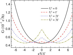
Figure 3: (color online) Differential conductance as a function of the bias voltage for different inter-dot interaction parameter $U^{\prime}$, as indicated in the figure. The other parameters are $k_{\rm B}T=0.1\Gamma$, $\varepsilon=-10\Gamma$, $U=20\Gamma$, $t=\Gamma$, and $p=0$.

Moreover, although the position of the two minima depends on the inter-dot correlation, its value is rather independent of $U^{\prime}$, see Fig. 3.

When considering the case of linear response, zero temperature and negligible inter-dot correlation, the minimum value of the differential conductance can be approximated by the following formula

$$G=\frac{e^{2}t^{2}\Gamma^{2}}{2h}\left[\frac{1}{\varepsilon^{2}}-\frac{1}{\varepsilon(\varepsilon+U)}+\frac{1}{(\varepsilon+U)^{2}}\right]^{2}\,.$$ (6)

For the parameters assumed to calculate Fig. 3, from the above formula one finds, $G=0.45\times 10^{-3}\;{\rm e^{2}/h}$, which is in good agreement with numerical results.

III.2 DQD coupled to ferromagnetic leads

If the leads are ferromagnetic ($p\neq 0$), the single-barrier second-order processes start to influence transport by affecting the DQD occupation probabilities. Transport characteristics are then a result of the interplay between processes driving the current and processes leading to spin relaxation in the dots. First, we note that the rate of single-barrier processes is proportional to temperature, while that of third-order processes depends on the applied bias voltage, see Eqs. (A) and (A). This will give rise to interesting phenomena, depending on the relative ratio of the second-order and third-order processes, as will be discussed in the following.

In Fig. 4 we show the bias dependence of the differential conductance for the parallel and antiparallel magnetic configurations of the system for several values of the inter-dot interaction parameter $U^{\prime}$. First of all, it can be seen that the value of $G$ at the zero bias increases with increasing the inter-dot correlation. This is a general feature which is present in both magnetic configurations of the system and gives rise to the zero-bias maximum, see Fig. 4a and b. The mechanism leading to such behavior was already discussed in the nonmagnetic case, i.e. a finite value of $U^{\prime}$ results in increased cotunneling through one-particle and two-particle virtual states, which in turn leads to an enhancement of the differential conductance at the zero bias.

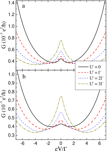
Figure 4: (color online) Bias dependence of the differential conductance in the parallel (a) and antiparallel (b) magnetic configurations for different inter-dot interaction parameter $U^{\prime}$, as indicated. The other parameters are $k_{\rm B}T=0.1\Gamma$, $\varepsilon=-10\Gamma$, $U=20\Gamma$, $t=\Gamma$, and $p=0.5$.

Another feature visible in the case of ferromagnetic leads is that even for negligible $U^{\prime}$ there is a small maximum in $G$ at the zero bias, irrespective of magnetic configuration of the system. This maximum bears a resemblance to the zero-bias anomaly found in the case of single quantum dots. weymannPRBBR05 However, in single quantum dots the maximum is present only in the antiparallel configuration, while in the case of double quantum dots, interestingly, the zero-bias peak is present in both magnetic configurations, see Fig. 4a and b. In order to understand this behavior we note that when there is a finite bias voltage applied to the system, a nonequilibrium spin accumulation can build up in the DQD. More precisely, for positive bias voltage in the parallel configuration one observes unequal occupation of singlet states, $P_{|\downarrow\uparrow\rangle}>P_{|\uparrow\downarrow\rangle}$, while triplets are roughly equally occupied (no spin accumulation), $P_{|\uparrow\uparrow\rangle}\approx P_{|\downarrow\downarrow\rangle}$. On the other hand, in the antiparallel configuration there is unequal occupation of triplet states (spin accumulation), $P_{|\downarrow\downarrow\rangle}>P_{|\uparrow\uparrow\rangle}$, whereas singlets are equally occupied, $P_{|\downarrow\uparrow\rangle}\approx P_{|\uparrow\downarrow\rangle}$. It is further interesting to realize that for positive bias voltage main contribution to the current comes from third-order tunneling processes having the initial state $|\uparrow\downarrow\rangle$ for the parallel and $|\uparrow\uparrow\rangle$ for the antiparallel magnetic configuration. Thus, with increasing the bias voltage ($V>0$), the contribution coming from those processes is decreased, leading to a decreased conductance. As a consequence, one observes a maximum at the zero bias even in the case of $U^{\prime}=0$, see Fig. 4.

The zero-bias maximum in differential conductance is therefore a result of superposition of two different effects. The first one concerns the asymmetry of cotunneling through virtual states, which is induced by a finite value of the inter-dot Coulomb interaction. Whereas the second one is associated with unequal occupation of the corresponding DQD states, which results from spin-dependent tunneling rates.

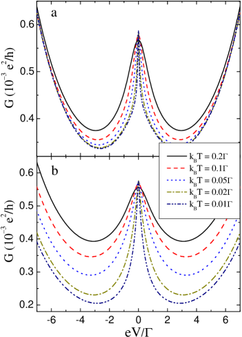
Figure 5: (color online) Bias dependence of the differential conductance in the parallel (a) and antiparallel (b) magnetic configurations for different temperatures and for $U^{\prime}=2\Gamma$. The other parameters are the same as in Fig. 4.

When the DQD is coupled to ferromagnetic leads, an important role is played by the single-barrier second-order processes – they do not contribute to the current, but lead to the spin relaxation in the double dot system. In order to gain more intuitive understanding of the discussed phenomena, in the following we present a crude quantitative analysis of the processes determining transport behavior. When considering the low temperature limit and assuming $U=-2\varepsilon$, $U^{\prime}=0$, the rate of single-barrier second-order processes can be approximated byweymannPRB06

$${\gamma^{(2)}}_{jj}^{|\sigma\chi\rangle\rightarrow|\bar{\sigma}\chi\rangle}\approx\frac{4k_{\rm B}T\Gamma^{2}}{h\varepsilon^{2}}\,.$$ (7)

On the other hand, we note that generally the fastest third-order processes are the ones leading to the change of the dot state from $|\sigma\bar{\sigma}\rangle$ into $|\bar{\sigma}\sigma\rangle$. With the same assumptions as made above, one can approximate the rate of such processes by the following formula

$${\gamma^{(3)}}_{jj^{\prime}}^{|\sigma\bar{\sigma}\rangle\rightarrow|\bar{\sigma}\sigma\rangle}\approx\frac{16|eV|t^{2}\Gamma^{2}}{h\varepsilon^{4}}\,.$$ (8)

The above expressions show explicitly that the relative ratio of both processes depends on the internal system parameters as well as the temperature and applied bias voltage. Furthermore, one can now roughly estimate the bias voltage at which the corresponding second-order and third-order processes become comparable, it is given by

$$|eV|\approx\frac{k_{\rm B}T\varepsilon^{2}}{4t^{2}}\,.$$ (9)

This formula will be helpful in discussing the temperature dependence of transport characteristics.

The influence of temperature on the bias dependence of differential conductance in both magnetic configurations is shown in Fig. 5. One can see that with increasing thermal energy, the width of the zero-bias peak is increased, while the maximum value of $G$ for $V=0$ stays rather unchanged. This is due to the fact that by raising the temperature, one increases the role of single-barrier second-order processes, see Eq. (7), giving rise to faster spin relaxation. Spin relaxation in turn leads to a decrease in the spin accumulation induced in the system. weymannPRB06 Therefore, the temperature effects on the differential conductance are more visible in the antiparallel configuration than in the parallel one. By decreasing $T$, the relative role of second-order processes is decreased, which leads to larger spin accumulation, $P_{|\downarrow\downarrow\rangle}>P_{|\uparrow\uparrow\rangle}$. This in turn gives rise to an increased and more robust drop of the differential conductance with the bias voltage, see for example the curves for $k_{\rm B}T=0.2\Gamma$ and $k_{\rm B}T=0.01\Gamma$ in Fig. 5. As a consequence, with decreasing temperature, the value of the differential conductance at the minimum is decreased and the width of the zero-bias peak becomes smaller – the two minima in $G$ appear at smaller bias voltage. This is due to the fact that the relative ratio of the second-order and third-order processes changes with changing $T$ and, consequently, the bias voltage at which the rates of these two processes are comparable is changed, see Eq. (9). The dependence of the differential conductance on temperature in the parallel configuration is less pronounced than in the antiparallel configuration because for the parallel configuration the single-barrier spin-flip processes only slightly affect the DQD occupations. This results from the fact that in the parallel configuration there is a left-right symmetry between the couplings to the spin-majority and spin-minority electron subbands. weymannPRBBR05

We also note that in the spinless case discussed in previous subsection the single-barrier second-order processes do not affect transport in any way, and the occupations of all DQD states are equal. Therefore, the differential conductance only slightly depends on temperature.

In Fig. 6 we present the TMR as a function of the bias voltage for several values of the inter-dot correlation parameter. First of all, it can be seen that for low bias voltages tunnel magnetoresistance is only slightly affected by the inter-dot interaction. This is due to the fact that the asymmetry in tunneling through virtual states induced by finite value of $U^{\prime}$ changes transport characteristics in both magnetic configurations in a similar way, see Fig. 4. As a consequence, the TMR, which reflects the difference between the parallel and antiparallel magnetic configuration, is roughly independent of the value of inter-dot correlation.

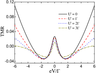
Figure 6: (color online) Bias dependence of the TMR for different inter-dot interaction parameter $U^{\prime}$ and for $k_{\rm B}T=0.1\Gamma$. The other parameters are the same as in Fig. 4.

Another interesting feature visible in Fig. 6 is the sign change of the TMR – with increasing the bias voltage, tunnel magnetoresistance decreases from a maximum at the zero bias to a minimum, at which TMR changes sign and becomes negative. At this bias voltage conductance in the parallel configuration is smaller than in the antiparallel configuration. This seemingly counterintuitive fact can be understood when one takes into account the effect of second-order processes giving rise to spin relaxation. As already mentioned, in the parallel configuration one finds, $P_{|\uparrow\downarrow\rangle}\neq P_{|\downarrow\uparrow\rangle}$, while in the antiparallel configuration one has, $P_{|\uparrow\uparrow\rangle}\neq P_{|\downarrow\downarrow\rangle}$. Spin relaxation processes decrease the spin accumulation in the antiparallel configuration, which leads to an enhancement of the differential conductance, see Fig. 5b. On the other hand, in the parallel configuration the DQD occupations only slightly depend on second-order processes. As a consequence, if the spin relaxation processes are sufficiently fast, ${\gamma^{(2)}}_{jj}^{|\sigma\chi\rangle\rightarrow|\bar{\sigma}\chi\rangle}\gtrsim{\gamma^{(3)}}_{jj^{\prime}}^{|\sigma\bar{\sigma}\rangle\rightarrow|\bar{\sigma}\sigma\rangle}$, one observes negative TMR effect.

In Fig. 7 we display the TMR effect as a function of the bias voltage for different temperatures. First of all, one can see that TMR exhibits a nontrivial dependence on temperature. This is because by changing $T$, one effectively changes the amount of processes leading to spin relaxation which affect spin accumulation and, thus, conductance in the antiparallel configuration. For low temperatures, second-order processes are suppressed and TMR becomes positive in the whole range of the bias voltage with a minimum at the zero bias, see the curve for $k_{\rm B}T=0.01\Gamma$ in Fig. 7. On the other hand, for higher temperatures the rate of single-barrier second-order processes is increased, which gives rise to two minima in the TMR separated by the zero-bias maximum, see Figs. 6 and 7. Moreover, at these minima TMR changes sign and becomes negative. We note that the negative TMR was also observed in single quantum dots in the limit of fast spin relaxation in the dot. weymannPRB06

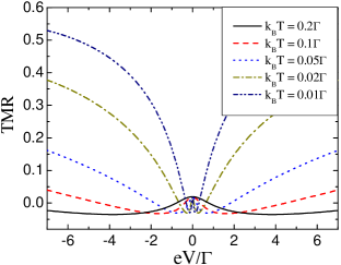
Figure 7: (color online) Tunnel magnetoresistance as a function of the bias voltage for different temperatures and for $U^{\prime}=2\Gamma$. The other parameters are the same as in Fig. 4.

Finally, we present analytical formulas approximating tunnel magnetoresistance in the most characteristic transport regimes. For $|eV|\gg k_{\rm B}T$, the TMR can be expressed as

$${\rm TMR}=\frac{2p^{2}}{1-p^{2}}\frac{53-3p^{2}(1+7p^{2}-p^{4})}{(5+3p^{2})(3-p^{2})^{2}}\,,$$ (10)

where we have assumed the symmetric Anderson model for each dot, $U=-2\varepsilon$, and $U^{\prime}=0$. This formula approximates the TMR in the zero temperature limit, i.e. in the absence of second-order processes. On the other hand, the linear response TMR calculated with the same assumptions can be approximated by

$${\rm TMR}=\frac{2p^{2}}{1-p^{2}}\frac{13+3p^{4}}{(9+p^{2})(5+3p^{2})}\,.$$ (11)

IV Concluding remarks

We have considered cotunneling transport through double quantum dots in series weakly coupled to ferromagnetic leads. In the Coulomb blockade regime the current flows through the system due to third-order tunneling processes. We have also taken into account the single-barrier second-order processes which do not contribute to the current but affect the DQD occupation probabilities.

We have shown that the differential conductance exhibits a maximum at the zero bias, irrespective of magnetic configuration of the system. This anomalous behavior results from the superposition of two different effects. The first effect is associated with asymmetry of cotunneling through different virtual states which can be induced by the inter-dot Coulomb interaction. The second mechanism results from the interplay of single-barrier second-order processes leading to spin relaxation and the third-order tunneling processes contributing to the current. The first mechanism does not depend on the value of spin polarization of the leads, the second one, on the contrary, results from the spin dependency of tunneling rates.

We have also analyzed the temperature dependence of transport characteristics. By changing thermal energy, one effectively changes the rate of the second-order processes, i.e. the amount of spin relaxation processes. We have shown that the width of the zero-bias maximum in the differential conductance increases with increasing temperature. This effect is most visible in the antiparallel configuration, which is due to the fact that in the antiparallel configuration spin relaxation decreases the spin accumulation induced in the DQD system, while occupations in the parallel configuration only slightly depend on the spin relaxation.

Furthermore, we have also shown that TMR exhibits a nontrivial dependence on temperature. For low temperatures, the TMR exhibits a minimum at the zero bias. However, for higher temperatures this minimum splits into two minima separated by a maximum at the zero bias. At the these minima tunnel magnetoresistance changes sign and becomes negative.

Appendix A Examples of cotunneling rates

In the following we present the explicit formulas for the third-order and second-order tunneling rates corresponding to processes shown in Fig. 2a and b. To determine the rate ${\gamma^{(3)}}^{|\downarrow\uparrow\rangle\rightarrow|\uparrow\uparrow\rangle}_{\rm LR}$ one needs to find the initial and final energies of the whole process, as well as the energies of the virtual states, as sketched in Fig. 2a. Then, by calculating the respective energy differences and plugging them into Eq. (3), one finds

$${\gamma^{(3)}}^{|\downarrow\uparrow\rangle\rightarrow|\uparrow\uparrow\rangle}_{\rm LR}=\frac{\Gamma_{\rm L}^{\uparrow}\Gamma_{\rm R}^{\downarrow}t^{2}}{h}\int d\omega f^{+}(\omega)f^{-}(\omega+\mu_{\rm L}-\mu_{\rm R})$$

$$\times\left[\frac{1}{(\omega+\mu_{\rm L}-\varepsilon-U-U^{\prime})^{2}}-\frac{1}{U-U^{\prime}}\right.$$

$$\left.\times\left(\frac{1}{\omega+\mu_{\rm L}-\varepsilon-U-U^{\prime}}-\frac{1}{\omega+\mu_{\rm L}-\varepsilon-U^{\prime}}\right)\right]^{2}\,,$$ (12)

where $f^{+}$ is the Fermi function and $f^{-}=1-f^{+}$. On the other hand, the single-barrier second-order rate for the process shown in Fig. 2b can be found in a similar way. This rate is given by

$${\gamma^{(2)}}^{|\uparrow\sigma\rangle\rightarrow|\downarrow\sigma\rangle}_{\rm LL}=\frac{\Gamma_{\rm L}^{\uparrow}\Gamma_{\rm L}^{\downarrow}}{h}\int d\omega f^{+}(\omega)f^{-}(\omega)$$

$$\times\left[\frac{1}{\omega+\mu_{\rm L}-\varepsilon-U-U^{\prime}}-\frac{1}{\omega+\mu_{\rm L}-\varepsilon-U^{\prime}}\right]^{2}\,.$$ (13)

We note that in the simplest approximation weymannEPJ05 for the Coulomb blockade regime one can pull out the resolvents in front of the integrals. Then, one arrives at the following integral, $\int d\omega f^{+}(\omega)f^{-}(\omega+\xi)$, where $\xi=\mu_{\rm L}-\mu_{\rm R}$ or $\xi=0$, correspondingly, which can be easily calculated. averin92 As a consequence, one can see that the rate of single-barrier second-order processes is proportional to temperature $T$, whereas that of the third-order processes depends on the bias voltage $V$.

References

- (1) K. Ono, D. G. Austing, Y. Tokura, and S. Tarucha, Science 297, 1313 (2002).
- (2) W. G. van der Wiel, S. De Franceschi, J. M. Elzerman, T. Fujisawa, S. Tarucha, and L. P. Kouwenhoven, Rev. Mod. Phys. 75, 1 (2003).
- (3) H. W. Liu, T. Fujisawa, T. Hayashi, and Y. Hirayama, Phys. Rev. B 72, 161305 (2005).
- (4) V. N. Golovach and D. Loss, Phys. Rev. B 69, 245327 (2004).
- (5) D. T. McClure, L. DiCarlo, Y. Zhang, H.-A. Engel, C. M. Marcus, M. P. Hanson, and A. C. Gossard, Phys. Rev. Lett. 98, 056801 (2007).
- (6) B. Wunsch, M. Braun, J. König, and D. Pfannkuche, Phys. Rev. B 72, 205319 (2005).
- (7) M. R. Gräber, W. A. Coish, C. Hoffmann, M. Weiss, J. Furer, S. Oberholzer, D. Loss, and C. Schönenberger, Phys. Rev. B 74, 075427 (2006).
- (8) E. Cota, R. Aguado, and G. Platero, Phys. Rev. Lett. 94, 107202 (2005).
- (9) B. L. Hazelzet, M. R. Wegewijs, T. H. Stoof, and Yu. V. Nazarov, Phys. Rev. B 63, 165313 (2001).
- (10) J. Fransson, M. Rasander, Phys. Rev. B 73, 205333 (2006).
- (11) J. Fransson, Nanotechnology 17, 5344 (2006).
- (12) J. Inarrea, G. Platero and A. H. MacDonald, cond-mat/0609323 (unpublished).
- (13) B. Muralidharan and S. Datta, cond-mat/0702161 (unpublished).
- (14) S. A. Wolf, D. D. Awschalom, R. A. Buhrman, J. M. Daughton, S. von Molnar, M. L. Roukes, A. Y. Chtchelka, and D. M. Treger, Science 294, 1488 (2001).
- (15) Semiconductor Spintronics and Quantum Computation, ed. by D.D. Awschalom, D. Loss, and N. Samarth (Springer, Berlin 2002).
- (16) S. Maekawa and T. Shinjo, Spin Dependent Transport in Magnetic Nanostructures (Taylor & Francis 2002).
- (17) I. Zutic, J. Fabian, S. Das Sarma, Rev. Mod. Phys. 76, 323 (2004).
- (18) S. Maekawa, Concepts in Spin Electronics (Oxford 2006).
- (19) D. Loss and D. P. DiVincenzo, Phys. Rev. A 57, 120 (1998).
- (20) A. C. Johnson, J. R. Petta, and C. M. Marcus, M. P. Hanson and A. C. Gossard, Phys. Rev. B 72, 165308 (2005).
- (21) H. I. Jorgensen, K. Grove-Rasmussen, J. R. Hauptmann, P. E. Lindelof, Appl. Phys. Lett. 89 232113 (2006).
- (22) S. Sapmaz, C. Meyer, P. Beliczynski, P. Jarillo-Herrero, Leo P. Kouwenhoven, Nano Lett. 6 (7), 1350 (2006).
- (23) M. R. Gräber, M. Weiss, C. Schönenberger, Semicond. Sci. Technol. 21, 64 (2006).
- (24) M. Julliere, Phys. Lett. A 54, 225 (1975).
- (25) J. Barnaś and A. Fert, Phys. Rev. Lett. 80, 1058 (1998).
- (26) S. Takahashi and S. Maekawa, Phys. Rev. Lett. 80, 1758 (1998).
- (27) B. R. Bułka, Phys. Rev. B 62, 1186 (2000).
- (28) W. Rudziński and J. Barnaś, Phys. Rev. B 64, 085318 (2001).
- (29) J. König and J. Martinek, Phys. Rev. Lett. 90, 166602 (2003).
- (30) M. Braun, J. König, J. Martinek, Phys. Rev. B 70, 195345 (2004).
- (31) I. Weymann, J. König, J. Martinek, J. Barnaś, and G. Schön, Phys. Rev. B 72, 115334 (2005).
- (32) I. Weymann, J. Barnaś, cond-mat/0611447 (to be published in Phys. Rev. B)
- (33) D. V. Averin and A. A. Odintsov, Phys. Lett. A 140, 251 (1989); D. V. Averin and Yu. V. Nazarov, Phys. Rev. Lett. 65, 2446 (1990).
- (34) K. Kang and B. I. Min, Phys. Rev. B 55, 15412 (1997).
- (35) D. V. Averin and Yu. V. Nazarov, in Single Charge Tunneling, edited by H. Grabert and M. Devoret (Plenum, New York 1992).
- (36) I. Weymann, J. Barnaś, J. König, J. Martinek, and G. Schön, Phys. Rev. B 72, 113301 (2005).
- (37) S. Braig and P. W. Brouwer, Phys. Rev. B 71, 195324 (2005).
- (38) I. Weymann, J. Barnaś, Eur. Phys. J. B 46, 289 (2005).
- (39) I. Weymann, J. Barnaś, Phys. Rev. B 73, 205309 (2006).
- (40) I. Weymann, Europhys. Lett. 76, 1200 (2006).
- (41) F. M. Souza, J. C. Egues, and A. P. Jauho, cond-mat/0611336 (unpublished).
- (42) J. Fransson, Europhys. Lett. 70, 796 (2005).
- (43) A. Kogan, S. Amasha, D. Goldhaber-Gordon, G. Granger, M.A. Kastner, and H. Shtrikman, Phys. Rev. Lett. 93, 166602 (2004).
- (44) Y. Chye, M. E. White, E. Johnston-Halperin, B. D. Gerardot, D. D. Awschalom, and P. M. Petroff, Phys. Rev. B 66, 201301(R) (2002).
- (45) M. M. Deshmukh and D. C. Ralph, Phys. Rev. Lett. 89, 266803 (2002).
- (46) H. B. Heersche, Z. de Groot, J. A. Folk, L. P. Kouwenhoven, and H. S. J. van der Zant, A. A. Houck, J. Labaziewicz, and I. L. Chuang, Phys. Rev. Lett. 96, 017205 (2006).
- (47) L. Y. Zhang, C. Y. Wang, Y. G. Wei, X. Y. Liu, and D. Davidović, Phys. Rev. B 72, 155445 (2005).
- (48) K. Tsukagoshi, B. W. Alphenaar, and H. Ago, Nature 401, 572 (1999).
- (49) B. Zhao, I. Mönch, H. Vinzelberg, T. Mühl, and C. M. Schneider, Appl. Phys. Lett. 80, 3144 (2002); J. Appl. Phys. 91, 7026 (2002).
- (50) A. Jensen, J. R. Hauptmann, J. Nygard, and P. E. Lindelof, Phys. Rev. B 72, 035419 (2005).
- (51) S. Sahoo, T. Kontos, J. Furer, C. Hoffmann, M. Gräber, A. Cottet, and C. Schönenberger, Nature Physics 1, 102 (2005).
- (52) A. N. Pasupathy, R. C. Bialczak, J. Martinek, J. E. Grose, L. A. K. Donev, P. L. McEuen, and D. C. Ralph, Science 306, 86 (2004).
- (53) A. Bernand-Mantel, P. Seneor, N. Lidgi, M. Munoz, V. Cros, S. Fusil, K. Bouzehouane, C. Deranlot, A. Vaures, F. Petroff, and A. Fert, Appl. Phys. Lett. 89, 062502 (2006).
- (54) K. Hamaya, S. Masubuchi, M. Kawamura, and T. Machida, M. Jung, K. Shibata, and K. Hirakawa, T. Taniyama, S. Ishida and Y. Arakawa, Appl. Phys. Lett. 90, 053108 (2007).
- (55) J. Aghassi, A. Thielmann, M. H. Hettler, G. Schön, Appl. Phys. Lett. 89, 052101 (2006); Phys. Rev. B 73, 195323 (2006).