A single atom in free space as a quantum aperture

Abstract

We calculate exact 3-D solutions of Maxwell equations corresponding to strongly focused light beams, and study their interaction with a single atom in free space. We show how the naive picture of the atom as an absorber with a size given by its radiative cross section $\sigma=3\lambda^{2}/2\pi$ must be modified. The implications of these results for quantum information processing capabilities of trapped atoms are discussed.

The resonant absorption cross section for a single two-state atom in free space driven by an electromagnetic field of wavelength $\lambda$ is $\sigma=3\lambda^{2}/2\pi$ [1]. Thus it seems reasonable to assume that a “weak” incident light beam focused onto an area $A\sim$ $\sigma$ would experience a loss (as resonance fluorescence) comparable to the incident energy of the beam itself and would, for off-resonant excitation, suffer an appreciable phase shift. In terms of nonlinear properties, note that the saturation intensity for a two-state atom in free space is $I_{s}=\hbar\omega_{a}/2\sigma\tau$, where $\omega_{a}$ is the atomic transition frequency and $\tau=1/\Gamma$ is the atomic lifetime. Hence, a single-photon pulse of duration $T\sim$ $\tau$ should provide a saturating intensity and allow for the possibility of nonlinear absorption and dispersion in a strong-focusing geometry.

These considerations suggest that a single atom in free space could perform important tasks relevant to quantum information processing, such as nonlinear entangling operations on single photons of different modes for the implementation of quantum logic, along the lines of Ref.  [2], but now without the requirement of an optical cavity [3]. Further motivation on this front comes from the need to address small quantum systems individually, as for example in the ion-trap quantum computer [4, 5] or in quantum communication protocols with trapped atoms in optical cavities [6, 7]. Here, each ion (or atom) must be individually addressed by focusing a laser beam with resolution $\Delta x\gtrsim\lambda$ [8]. Interesting effects may also be expected with respect to the photon statistics of the scattered light in a regime of strong focusing, such as extremely large photon bunching [9]. Conversely, alterations of atomic radiative processes arising from excitation with squeezed and other forms of nonclassical light would be feasible as well [10]. Finally, questions of strong focusing become relevant for dipole-force traps of size $\lambda$ for single atoms.

Against this backdrop of potential applications, we note that radiative interactions of single atoms with strongly focused light beams have received relatively little attention. Indeed, previous experiments have been restricted to a regime of weak focusing and resultingly small fractional changes in transmission [11, 12, 13], either because of large focal spot size $\sim 1000\lambda^{2}$ [12] or reduced oscillator strengths for molecular transitions [13]. On the theoretical front, we recall only Refs. [9] studying the photon statistics by adopting a quasi one-dimensional model.

In light of its fundamental importance, in this Letter we report the first complete 3-dimensional calculations for the interaction of strongly focused light beams and single atoms in free space. Essential elements in this work are exact 3-D vector solutions of Maxwell equations that represent beams of light focused by a strong spherical lens. As an application of our formalism, we calculate the scattered intensities and the intensity correlation function $g^{(2)}(0,\vec{r})$ as functions of angle for resonant excitation of a single atom with a strongly focused beam. We find an intriguing interplay between the angular properties of the scattered light and its quantum statistical character (e.g., photon bunching and antibunching versus scattering angle), leading to the concept of a quantum aperture. Our results, in particular those corresponding to scattering in the forward direction, are compared to those of Ref.  [9], and to similar calculations using 3-dimensional paraxial Gaussian beams [14], which we find do not always represent the actual situation with strongly focused light beams.

We start by constructing exact solutions of the Maxwell equations describing tightly focused beams (a detailed analysis is deferred to [15], see also [16]). An incoming (paraxial) beam with fixed circular polarization $\vec{\epsilon}_{+}=(\hat{x}+i\hat{y})/\sqrt{2}$ and frequency $\omega$ propagates in the positive $z$ direction and illuminates an ideal lens. The incoming beam is taken to be a lowest-order Gaussian beam with Rayleigh range $z_{{\rm in}}$ with $kz_{{\rm in}}\gg 1$, and is characterized by the dimensionless amplitude

$$\vec{F}_{0}=\exp\left(-\frac{k\rho^{2}}{2z_{{\rm in}}}\right)\vec{\epsilon}_{+},$$ (1)

where $\rho$ is the distance to the $z$ axis and the wave vector $k=2\pi/\lambda$. For simplicity the focal plane of the incoming beam and the plane of the lens are taken to coincide. After transforming this input field through the lens, the output field behind the lens is expanded in a complete set of modes $\vec{F}_{\mu}$ that are exact solutions of the source-free Maxwell equations adapted to the cylindrical symmetry of the problem, as constructed in [17]. The index $\mu$ is short-hand for the set of mode numbers $\mu=(k_{t},m,s)$, with $k_{t}$ the transverse momentum number $k_{t}=(k^{2}-k_{z}^{2})^{1/2}$, $s$ the polarization index and $m$ a topological index related to orbital angular momentum [17]. For fixed $k$, the dimensionless mode functions $\vec{F}_{\mu}$ are normalized to

$$\int_{z={\rm const}}{\rm d}S\vec{F}_{\mu}^{*}\cdot\vec{F}_{\nu}=\delta(k_{t}-k_{t}^{\prime})\delta_{mm^{\prime}}\delta_{ss^{\prime}}/(2\pi k_{t}).$$ (2)

As for the field transformation by the lens, the action of a spherical lens is modeled by assuming that the field distribution of the incoming field is multiplied by a local phase factor $\exp(-ik\rho^{2}/2f)$, with $f$ the focal length of the lens [18]. Thus, if in the plane of the lens, say $z=0$, the incoming beam is given by $\vec{F}_{{\rm in}}=\vec{F}_{0}$ as above, then the output field is given by

$$\vec{F}_{{\rm out}}(\vec{r})=\int{\rm d}k_{t}\sum_{m}\sum_{s}\kappa_{\mu}\vec{F}_{\mu}(\vec{r}),$$ (3)

where for the particular choice of $\vec{F}_{0}$, $\kappa_{\mu}$ is [15]

$$\kappa_{\mu}=\pi\delta_{m1}\frac{k_{t}}{k}\frac{k_{z}+sk}{k}\xi\exp\left(-\frac{k_{t}^{2}}{2k}\xi\right),$$ (4)

with $\xi\equiv z_{R}-iz_{0}$, and

$$z_{R}=\frac{f^{2}z_{{\rm in}}}{z_{{\rm in}}^{2}+f^{2}},\text{ \ }z_{0}=\frac{fz_{{\rm in}}^{2}}{z_{{\rm in}}^{2}+f^{2}}.$$ (5)

In general, the expression (3) for the outgoing field must be evaluated numerically. In the paraxial limit, when $kz_{R}\gg 1$, $z_{R}$ and $z_{0}$ correspond to the Rayleigh range and the position of the focal plane of the outgoing beam, respectively.

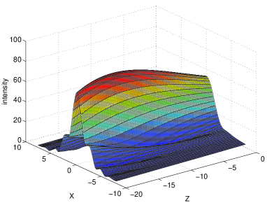
FIG. 1.: Surface plot of the relative intensity $|\vec{F}_{{\rm out}}\cdot\vec{\epsilon}_{+}|^{2}$ of a strongly focused beam as a function of the dimensionless axial coordinate $Z\equiv(z-z_{0})/\lambda$ and transverse coordinate $X\equiv x/\lambda$. The lens is located at $z=0$ and is characterized by $f=500\lambda$, with the incoming Gaussian beam having $z_{{\rm in}}/\lambda=6\times 10^{4}$. This implies $z_{0}\approx 500\lambda$ and $z_{R}\approx 4.2\lambda$. For paraxial beams, the focal plane would be at $Z=0$.

A particular result for the $\vec{\epsilon}_{+}$ component of $\vec{F}_{{\rm out}}(\vec{r})$ in the focal region is given in Fig. 1. Note that the focal plane deviates from the paraxial result $z=z_{0}$ and moves towards the lens by several wavelengths. Furthermore, the size of focal spot for the exact light beam is larger than the corresponding value $\pi w_{R}^{2}$ with $w_{R}\equiv\sqrt{z_{R}\lambda/\pi}$ for a paraxial beam.

With these results in hand, we now investigate the response of an atom located at a position $\vec{r}_{0}$ in the focal spot (i.e. the position of maximum field intensity) of a strongly focused light beam as in Figure 1. The goal is to identify the “maximum” effect that such an atom can have on the transmitted and scattered fields. We consider a $J_{g}=0\rightarrow J_{e}=1$ transition in the atom, as it is the simplest case where all three polarization components of the light in principle play a role. For the cases presented here with the atom located on the $z$ axis, the other two polarization components vanish [17], but they can play a dominant role in other situations.

To calculate mean values of the scattered field as well as its intensity and photon statistics, it is convenient to work in the Heisenberg picture, in which the electric field operator can be written as the sum of a “free” part and a “source” part, $\vec{E}=\vec{E}_{f}+\vec{E}_{s}$. The source part for the case of a $J_{g}=0\rightarrow J_{e}=1$ transition is given by [19]

$$\vec{E}_{s}^{(+)}(\vec{r})=\sum_{i}\vec{\Psi}_{i}(\vec{r}^{\prime})\sigma_{i}^{-}(t-|\vec{r}^{\prime}|/c).$$ (6)

We have separated the fields into positive- and negative-frequency components, $\vec{E}_{f,s}=\vec{E}_{f,s}^{(+)}+\vec{E}_{f,s}^{(-)}$, $\vec{r}^{\prime}=\vec{r}-\vec{r}_{0}$, $\sigma_{i}^{-}$ is the atomic lowering operator, and the sum is over three independent polarization directions $i=\pm 1,0$. In the far field, $\vec{\Psi}_{i}(\vec{r})$ is the dipole field

$$\vec{\Psi}_{i}(\vec{r})=\frac{\omega_{a}^{2}}{4\pi\varepsilon_{0}c^{2}}\left[\frac{\vec{d}_{i}}{r}-\frac{(\vec{d}_{i}\cdot\vec{r})\vec{r}}{r^{3}}\right].$$ (7)

Here $\vec{d}_{i}=d\hat{u}_{i}$ is the dipole moment between the ground state $|g\rangle$ and excited state $|e_{i}\rangle$ in terms of the unit circular vectors $\hat{u}_{i}$ and the reduced dipole matrix element $d$.

Expressions containing the electric field in time-ordered and normal-ordered form (as relevant to standard photo-detectors) can be transformed into “${\cal O}$-ordered form”, where $\vec{E}_{s}^{(+)}$ is placed to the left of $\vec{E}_{f}^{(+)}$, $\vec{E}_{f}^{(-)}$ to the left of $\vec{E}_{s}^{(-)}$, and where the source parts are time-ordered[19]. For instance, if we assume the initial state of the field incident upon the lens is a coherent state, then the normally ordered intensity $I(t,\vec{r})\equiv\langle\vec{E}^{(-)}(t,\vec{r})\cdot\vec{E}^{(+)}(t,\vec{r})\rangle$ can be written as the sum of three terms, the intensity $I_{d}\equiv\langle\vec{E}_{s}^{(-)}\cdot\vec{E}_{s}^{(+)}\rangle$ of the dipole field, the intensity $I_{L}\equiv\langle\vec{E}_{f}^{(-)}\cdot\vec{E}_{f}^{(+)}\rangle$ of the free (laser) field, and the interference term between the two fields. Similarly, the second-order correlation function $G^{(2)}(t,\tau,\vec{r})\equiv\sum_{l,m=x,y,z}\langle E_{l}^{(-)}(t)E_{m}^{(-)}(t+\tau)E_{m}^{(+)}(t+\tau)E_{l}^{(-)}(t)\rangle$ (where the dependence of the fields on $\vec{r}$ is suppressed) consists of 16 terms. For $\tau=0$, $7$ of these vanish, yielding

$$G^{(2)}(t,0,\vec{r})=|\alpha|^{4}|\vec{F}_{{\rm out}}|^{4}+2\sum_{i,j}|\alpha|^{2}|\vec{F}_{{\rm out}}|^{2}\vec{\Psi}_{i}^{\ast}\cdot\vec{\Psi}_{j}\sigma_{ee}^{ij}(t_{r})$$ (8)

$$+4\sum_{i}{\rm Re}(\alpha^{\ast}\exp(i\omega_{a}t))\vec{F}_{{\rm out}}^{\ast}\cdot\vec{\Psi}_{i}|\alpha|^{2}|\vec{F}_{{\rm out}}|^{2}\sigma_{eg}^{i}(t_{r}))$$ (9)

$$+2\sum_{i,j}|\alpha|^{2}(\vec{F}_{{\rm out}}\cdot\vec{\Psi}_{i}^{\ast})(\vec{F}_{{\rm out}}^{\ast}\cdot\vec{\Psi}_{j}\sigma_{ee}^{ij}(t_{r})),$$ (10)

where the coherent state amplitude is chosen such that $\langle\vec{E}_{f}^{(-)}\rangle=\alpha\vec{F}_{{\rm out}}$, $t_{r}$ is the retarded time $t_{r}=t-|\vec{r}^{\prime}|/c$, and $\sigma_{eg}^{i}=\langle\sigma_{i}^{-}\rangle$ and $\sigma_{ee}^{ij}=\langle\sigma_{i}^{+}\sigma_{j}^{-}\rangle$ are expectation values of the corresponding atomic operators.

To proceed beyond this point, we must evaluate the various atomic quantities. As a simple starting point and in order to make contact with the work of Ref. [9], we assume that the atom reaches a stationary steady state. In this case, given the value of the electric field at the atom’s position $\alpha\vec{F}_{{\rm out}}(\vec{r}_{0})$, the various atomic expectation values can be straightforwardly derived [19].

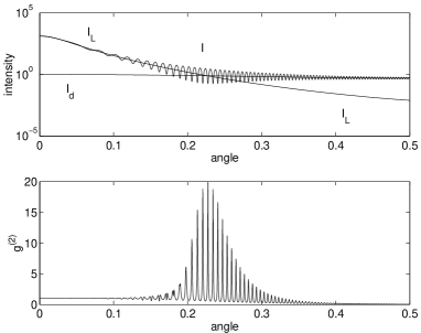
FIG. 2.: The intensities $I_{L}$ of the laser (free) field, $I_{d}$ of the dipole (source) field and $I$ of the total field relative to $I_{d}(\phi=0)$ as a function of the azimuthal angle $\phi/\pi$, (i.e, at position $\vec{r}=[R\sin\phi,0,R\cos\phi]$ where we chose $R=50\lambda$ here and for all further calculations). The parameters for the incoming beam and the lens are as in Fig. 1, and we chose $\lambda=852$nm, corresponding to the D2 transition in Cs. The atomic dipole moment $d$ is adjusted to give the corresponding spontaneous emission rate $\Gamma=2\pi\times 5$MHz for the 6$P_{3/2}$ states of Cs. (b) $g^{(2)}(0,\vec{r})$ as a function of $\phi/\pi$.

For weak ($\alpha\rightarrow 0$) on-resonance excitation, we have explicitly evaluated the scattered intensities as well as the normalized second-order correlation function $g^{(2)}(\tau,\vec{r})\equiv G^{(2)}(\tau,\vec{r})/I^{2}(\vec{r})$ at $\tau=0$ as functions of position in the far field. Recall that for a stationary steady state, there is no dependence on $t$. As can be seen in Figure 2a, in the forward direction (around $\phi=0$), the free-field contribution $\vec{E}_{f}$ from the forward propagating incident field overwhelms the source field contribution $\vec{E}_{s}$ from the atom, even for focusing to a spot of diameter $w_{R}\approx\lambda$ as in the figure (and in fact is true for any width). This may be compared to a similar result for classical scattering from spherical dielectrics with light focused down to spot sizes larger than 5 times the size of the spheres [20]. Not surprisingly then, we find that $g^{(2)}(0,\vec{r})\approx 1$ for forward scattering ($\phi\sim 0$) for any input beam, which, however, is in sharp contrast with the result from [9] which would predict a large bunching effect (i.e., $g^{(2)}\gg 1$) for sufficiently tight focusing. If we move instead to large angles ($\phi\sim\pi/2$), Figure 2a shows that the dipole field $\vec{E}_{s}$ dominates $\vec{E}_{f}$, so that $g^{(2)}(0,\vec{r})=0$ for $\phi\rightarrow\pi/2$ (i.e., the light is almost purely fluorescence and hence anti-bunched as for plane-wave excitation [21]).

The behavior of $g^{(2)}$ is most interesting around the angle $\phi_{0}$ where the incident $\vec{E}_{f}$ and source $\vec{E}_{s}$ fields have the same magnitude. Indeed, the oscillations apparent in Figure 2b indicate that $g^{(2)}(0,\vec{r})$ is very sensitive to the relative phase between $\vec{E}_{f}$ and $\vec{E}_{s}$. In fact, maxima in $g^{(2)}$ appear when the free field and the dipole field interfere destructively, which implies that the total field is smaller than the contribution from the incident field. Adopting the interpretation of Carmichael and Kochan [9] from an essentially one-dimensional setting to the angular dependence of the fields around $\phi_{0}$, we see that this implies that a photon has just been absorbed by the atom, which is therefore in its excited state, so that a fluorescent photon can be expected to appear soon, thus leading to strong bunching. We suggest that the combined angular dependences of $I(\vec{r})$ and $g^{(2)}(0,\vec{r})$ evidenced in Figure 2 are characteristic of scattering from a quantum aperture such as an atom in free space.

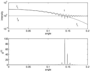
FIG. 3.: As Fig. 2, but for a paraxial beam characterized by the same beam parameters $z_{R}=4.2\lambda$ and $z_{0}=500\lambda$.

We have compared these exact 3-D results with those for a Gaussian beam with the same parameters $z_{0}$ and $z_{R}$. In qualitative terms, a Gaussian beam exaggerates the amount of light in the forward direction at the cost of greatly underestimating it for larger angles. This implies that the region where $g^{(2)}$ reaches its maximum is moved to smaller angles $\phi$ for a paraxial beam as compared to the exact result (for the parameters of Figure 2, $\phi_{0}\sim 26^{o}$ compared to $\phi_{0}\sim 40^{o}$, resp.). Moreover, the value of that maximum is exaggerated as well, with a maximum value of $g^{(2)}(0,\vec{r})\sim 100$ for the Gaussian beam. For even stronger focusing, there will be large bunching at $\phi=0$ for a paraxial beam, as in [9], but, as mentioned before, not for the exact solutions.

Finally, we come back to the issue raised at the beginning of this paper: why doesn’t focusing a light beam to size $\sigma$ give rise to large effects? One simple answer is of course that there is a limit to how strongly one can focus a light beam [22], as indeed our exact solutions show with focal areas $A$ always larger than $\sigma$. Moreover, for tightly focused beams, the polarization state in the focal volume is anything but spatially uniform so that the field associated with a single polarization for a paraxial input is split among various components. In fact, if the atomic dipole is $\vec{d}=d\hat{u}$, then the relevant quantity determining the excitation probability is $|\hat{u}\cdot\vec{E}^{(-)}(\vec{r}_{0})|^{2}$ evaluated at the atom’s position $\vec{r}_{0}$, while the total intensity in the focal plane is given by $\int{\rm d}S|\vec{E}^{(-)}|^{2}$. Thus, instead of $R=\sigma/A$, the scattering ratio $R_{s}$ is

$$R_{s}=\frac{3\lambda^{2}|\hat{u}\cdot\vec{E}^{(-)}(\vec{r}_{0})|^{2}}{2\pi\int{\rm d}S|\vec{E}^{(-)}|^{2}}.$$ (11)

For a paraxial beam $R_{s}=2\sigma/(\pi w_{R}^{2})\ll 1$. For the lens parameter used here, $f=500\lambda$, the optimum value (i.e., optimized over the parameters of the incoming beam) for $R_{s}$ is $10\%$. Note that the ratio of the intensities of scattered ($\vec{E}_{s}$) and laser fields ($\vec{E}_{f}$) in the forward direction ($\phi=0$ in Fig. 2) is much smaller than that (about $10^{-3}$), because the laser beam channels much more power in that direction than does the dipole field.

For extreme values of $f$ on the order of $\lambda$, the maximum scattering ratio does increase, but not beyond $50\%$. Even for a scattering ratio of close to 50% (reached for $f=2\lambda$ and $z_{{\rm in}}=4\lambda$, for instance), the ratio of laser field intensity $I_{L}$ to scattered intensity $I_{d}$ in the forward direction ($\phi=0$) is not small, namely about 21. Moreover, the value for $g^{(2)}(\tau=0)=0.95$ agrees with Ref. [9] in the sense that for the parameter $\Gamma\approx 0.5$ from that paper antibunching is indeed predicted. On the other hand, it is in contrast with the suggestion made there that very strong bunching results for focusing to an area $A\sim\sigma$. Finally, note that the upper limit of 50% for $R_{s}$ can be understood by noting that the optimum shape of the illuminating field would be a dipole field. Here with light coming only from one direction, one may indeed expect $R_{s}$ to be at most 0.5. With one mirror behind the atom, an improvement in the scattering ratio by about a factor of 2 might be expected. And of course, by building an optical cavity around the atom, the atom-light interaction can be further enhanced by orders of magnitude as in cavity quantum electrodynamics [23].

In conclusion, by strongly focusing light on a single atom in free space, one may indeed create an appreciable light-atom interaction. However, this interaction is not as strong as might be naively expected. On the one hand, this implies that a coherent-state field employed for “classical” addressing of a single atom in implementations of quantum computing and communication [4, 6, 7] carries little information about that atom, so that entanglement of the atom with other atoms in a quantum register can be preserved [15]. On the other hand, our analysis implies that there are serious obstacles associated with using a single atom in free space to process quantum information encoded in single photons.

We thank R. Legere for discussions. The work of HJK is supported by the Division of Chemical Science, Office of Basic Energy Science, Office of Energy, U.S. Department of Energy. SJvE is funded by DARPA through the QUIC (Quantum Information and Computing) program administered by the US Army Research Office, the National Science Foundation, and the Office of Naval Research.

REFERENCES

- [1] J.D. Jackson, Classical Electrodynamics (Wiley, New York, 1999).
- [2] S.L. Braunstein, C.M. Savage and D.F. Walls, Opt. Lett. 15, 628 (1990).
- [3] Q.A. Turchette et al., Phys. Rev. Lett. 75, 4710 (1995).
- [4] J.I. Cirac and P. Zoller, Phys. Rev. Lett. 78, 3221 (1995).
- [5] D.J. Wineland et al. J. Res. Natl. Inst. Stand. Technol. 103, 259 (1998).
- [6] J.I. Cirac et al., Phys. Rev. Lett. 78, 3221 (1997).
- [7] S.J. van Enk, J.I. Cirac and P. Zoller, Phys. Rev. Lett. 78, 4293 (1997).
- [8] H.C. Nägerl et al., Phys. Rev. A 60, 145 (1999).
- [9] H.J. Carmichael, Phys. Rev. Lett. 70, 2273 (1993); P. Kochan and H.J. Carmichael, Phys. Rev. A 50, 1700 (1994).
- [10] C.W. Gardiner and A.S. Parkins, Phys. Rev. A 50, 1792 (1994).
- [11] B. W. Peuse, M. G. Prentiss, and S. Ezekiel, Phys. Rev. Lett.74, 269 (1982).
- [12] D.J. Wineland, W.M. Itano and J.C. Bergquist, Opt. Lett. 12, 389 (1987).
- [13] W.E. Moerner and T. Basché, Angew. Chem. Int. Ed. Engl. 32, 457 (1993) and references therein.
- [14] A.E. Siegman, Lasers (University Science Book, Mill Valley, 1986).
- [15] S.J. van Enk and H.J. Kimble, unpublished.
- [16] G.P. Karman et al., J. Opt. Soc. Am. A 15, 884 (1998).
- [17] S.J. van Enk and G. Nienhuis, J. Mod. Optics 41, 963 (1994).
- [18] J.W. Goodman, Introduction to Fourier Optics (Van Nostrand, New York, 1968).
- [19] W. Vogel and D.-G Welsch, Lectures on Quantum Optics, Akademie Verlag GmbH, Berlin (1994).
- [20] J.T. Hodges et al., Appl. Optics 34, 2120 (1995).
- [21] H.J. Carmichael and D.F. Walls, J. Phys. B 9, L43 (1976); H.J. Kimble and L. Mandel, Phys. Rev. A 13, 2123 (1976).
- [22] For recent progress on focusing light beams see T.R.M. Sales, Phys. Rev. Lett. 81, 3844 (1998).
- [23] Cavity Quantum Electrodynamics, Adv. At. Mol. Opt. Physics, Suppl. 2, Ed. P.R. Berman (Academic Press, Boston, 1994).