Non-maximally entangled states: production, characterization and utilization

Abstract

Using a spontaneous-downconversion photon source, we produce true non-maximally entangled states, i.e., without the need for post-selection. The degree and phase of entanglement are readily tunable, and are characterized both by a standard analysis using coincidence minima, and by quantum state tomography of the two-photon state. Using the latter, we experimentally reconstruct the reduced density matrix for the polarization. Finally, we use these states to measure the Hardy fraction, obtaining a result that is $122\sigma$ from any local-realistic result.

Entanglement is arguably the defining characteristic of quantum mechanics, and can occur between any quantum systems, be they separate particles [1] or separate degrees of freedom of a single particle [2]. The latter can be used to realize interference-based all-optical implementations of quantum algorithms [3], while multi-particle entangled states are central in discussions of locality [4, 5], and in quantum information, where they enable quantum computation [6], cryptography [7], dense coding [8], and teleportation [9]. More generally, entanglement is the underlying mechanism for measurements on, and decoherence of, quantum systems, and thus is central to understanding the quantum/classical interface.

Historically, controlled production of multi-particle entangled states has proven to be non-trivial. To date, the “cleanest” and most accessible source of such entanglement arises from the process of spontaneous optical parametric downconversion in a nonlinear crystal (for a review, see [10]). This entanglement is of a specific and limited kind: the states are maximally entangled, e.g., $(|\rm{HV}\rangle\pm\varepsilon|\rm{VH}\rangle)/\sqrt{1+|\varepsilon|^{2}}$, where H and V respectively represent the horizontal and vertical polarizations of two separated photons, and $\varepsilon=1$. There is no possibility of varying the intrinsic degree of entanglement, $\varepsilon$ [11], to produce non-maximally entangled states without compromising the purity of the state, i.e., introducing mixture [12]. Non-maximally entangled states have been shown to reduce the required detector efficiencies for loophole-free tests of Bell inequalities [13], as well as allowing logical arguments that demonstrate the nonlocality of quantum mechanics without inequalities [14, 15, 16]. More generally, such states lie in a previously inaccessible range of Hilbert space, and may therefore be an important resource in quantum information applications.

States with a fixed degree of entanglement, $\varepsilon\simeq 4/3$, have been deterministically generated in ion traps [17], and there have been several optical experiments where non-maximally entangled states were controllably generated via post-selection, i.e., selective measurement of a product state, after the state had been produced [18, 19]. The latter experiments are of considerable pedagogical interest in that they demonstrate the logic behind inequality-free locality tests. However, the underlying state is factorizable, and so is not truly entangled. In this letter, we describe the controllable production, characterization, and utilization of true non-maximally entangled states, generated without postselection.

A detailed description of the downconversion source is given in [20]. In brief, it consists of two thin, adjacent, nonlinear optical crystals (beta-barium-borate, BBO), cut for Type-I phase matching. The crystals are aligned so that their optic axes lie in planes perpendicular to each other. The pump beam and optic axis of the first crystal define the vertical plane, that of the second crystal, the horizontal plane, see Fig. 1a. If the pump beam is vertically (horizontally) polarized, down conversion occurs only in crystal 1 (crystal 2). When the pump polarization is set to 45^∘, it is equally likely to downconvert in either crystal [21]. Given the coherence and high spatial overlap between these two processes, the photons are created in the maximally entangled state $(|\rm{HH}\rangle+e^{i\phi}|\rm{VV}\rangle)/\sqrt{2}$

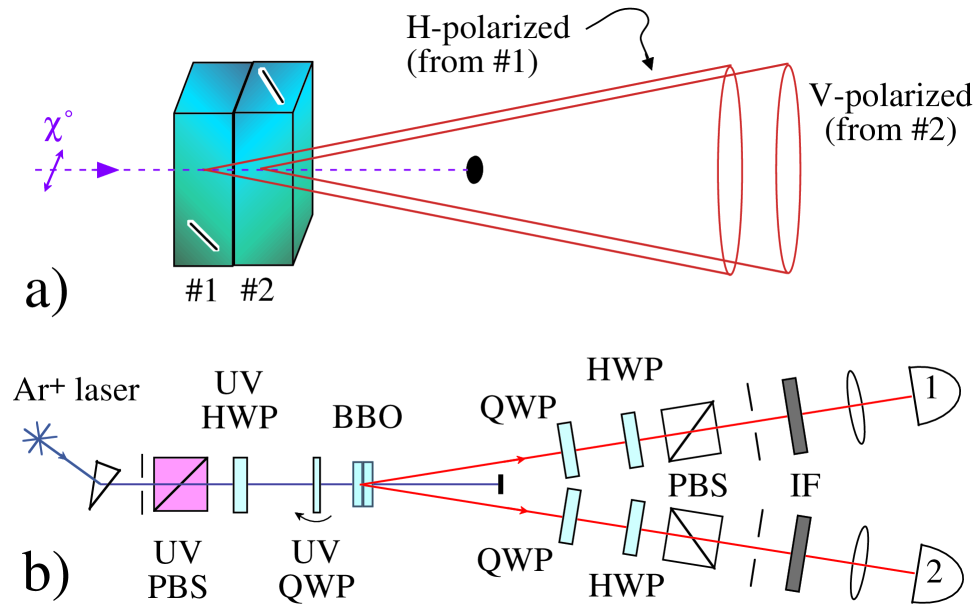
FIG. 1.: a) Non-maximal entanglement source. Twin photons are emitted along cones that originate at two identical down-conversion crystals, pumped by a 351 nm laser. The crystals are oriented so that the optic axis of the first (second) lies in the vertical (horizontal) plane. b) Experimental setup (top view) to pump and characterize the source. The pump beam is wavelength and polarization filtered via a prism and polarizing beamsplitter (UV PBS), respectively. The polarization is set by a half-wave plate (UV HWP).

where $\phi$ is adjusted via the ultra-violet quarter-wave plate (UV QWP) shown in Fig. 1b. Adjustable quarter- and half-wave plates (QWP & HWP) and polarizing beamsplitters (PBS), in the two downconversion beams, allow polarization analysis in any basis, i.e., at any position on the Poincaré sphere [22]. Each detector assembly comprised: an iris and a narrowband interference filter (IF, 702 nm $\pm$ 2.5 nm), to reduce background and select (nearly-) degenerate photons; a 35 mm focal length lens; and a single photon counter (EG&G SPCM-AQ). The detector outputs were recorded singly, and in coincidence using a time to amplitude converter and a signal-channel analyzer. A coincidence window of 5.27 ns was sufficient to capture true coincidences; since the resulting rate of accidental coincidences was negligible ($\sim$0.4s^-1), no corrections for this were necessary.

Non-maximally entangled states are produced simply by rotating the pump polarization. For a polarization angle of $\chi$ with respect to the vertical, the output state is, $|\psi\rangle=(|\rm{HH}\rangle+\varepsilon e^{i\phi}|\rm{VV}\rangle)/\sqrt{1+\varepsilon^{2}}$, where the degree of entanglement, $\varepsilon=\rm{tan}\ \chi$ [21]. The probability of coincident detection depends on the analyzer orientations:

$$\rm{P}_{12}(\theta_{1},\theta_{2}) = |\langle\theta_{1}|\langle\theta_{2}|\psi\rangle|^{2}$$ (1)

$$= |\rm{cos}\theta_{1}\ \rm{cos}\theta_{2}+\varepsilon e^{i\phi}\ \rm{sin}\theta_{1}\ \rm{sin}\theta_{2}|^{2}/(1+\varepsilon^{2}),$$ (2)

where for the moment we restrict ourselves to linear analyzers (i.e., by not using the QWP’s) and $\theta_{i}$ is the orientation of the linear polarizer in arm $i$, with respect to the vertical. Traditionally, maximally entangled states are analyzed by keeping one analyzer fixed and varying the other; the visibility and phase of the resulting fringes accurately characterize the state (with this source we recently attained visibilities of better than 99% [20]).

A related analysis method is to map out the coincidence probability function, in particular the distribution of the coincidence minima [19]. Solving for $\rm{P}_{12}(\theta_{1},\theta_{2})=0$, with $\phi=0$, we obtain $\rm{tan}\ \theta_{2}=-(\rm{cot}\ \theta_{1})/\epsilon$. The shape and orientation of the resulting curves indicate the degree and sign of the entanglement. Experimentally, the coincidences are not actually zero: the value of the minima are a measure of the state purity. Coincidence minima were found for a variety of states and analyzer settings, and fell in the range 0.2-1.0%, indicating very high purities. As Fig. 2 shows, across a wide range of entanglement there is good agreement between the experimentally determined coincidence minima and the above equation. However, the data towards the bottom and the right of the plot are pulled off the curves slightly. For states solely of the form $|$HH$\rangle$+$\varepsilon|$VV$\rangle$, this should not occur; however, close examination of our raw data shows there are small components of $|$HV$\rangle$ and $|$VH$\rangle$, even in the maximally entangled case. These components become proportionally more important as the state becomes less entangled. What is needed then, is an exact measurement of all components of the state, one that does not require any ana-

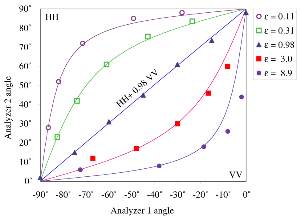
FIG. 2.: Coincidence minima for a spectrum of non-maxim- ally entangled states. points: experimentally determined coincidence minima, with uncertainties of $\pm 0.5^{\circ}$ (not shown); curves: predicted settings for zero coincidences, see text.

lytical assumptions.

Quantum state tomography is the solution. For continuous variables, tomography has been implemented in both quantum [23] and atom [24] optics. Tomography is also possible with discrete variables [25]. For example, the Stokes parameters, which characterize the mean polarization of a classical beam [26], directly yield the polarization density matrix for an ensemble of identically-prepared single photons [27]. To characterize our entangled states, we introduce the analogous two-photon Stokes parameters, which describe the photon polarization correlations in various bases. How many two-photon Stokes parameters are there? A pure state in $d$-dimensional Hilbert space is determined by 2$d$-2 linearly independent parameters, so only 2 and 6 parameters are respectively needed for the pure single and two-photon cases. In general, however, the state may be partially-mixed, and $d^{2}$-1 parameters are required for a full analysis. Thus 3 and 15 analyzer settings are respectively required to obtain the single- [28] and two-photon Stokes parameters. In fact, we use 16 analyzer settings, as listed in Table 1 (the extra setting determines the normalization). This is just one possible set; we will give a detailed discussion of discrete-variable tomography elsewhere, including extension to higher orders. Briefly, we define a probability vector, P, where the elements are the 16 coincidence counts normalized by the total coincidence rate (given by the sum of the first four measurements), and an invertible square matrix, M, which is derived from the measurement settings. The vector, M^-1.P, contains the real and imaginary components of the density matrix, $\hat{\rho}$. Elsewhere we discuss the implications of measurement drift and uncertainty; for the moment we simply note that there are small uncertainties in the final reconstructed density matrix. The density matrices for a spectrum of entangled states are shown in Fig. 3 [29].

TABLE I.: Settings for measuring two-photon Stokes parameters. H, V, and D are respectively horizontal, vertical, and diagonal (45^∘) linear polarization, L and R are left- and right-circular polarization. Shown are data for the near-maximally entangled state of Fig. 3a (counted over 100s).

analyzer	analyzer	coinc.	analyzer	analyzer	coinc.
in arm 1	in arm 2	count	in arm 1	in arm 2	count
H	H	34749	D	D	32028
H	V	324	R	D	15132
V	H	444	R	L	33586
V	V	35805	D	R	17932
H	D	17238	D	V	13441
H	L	16722	R	V	17521
D	H	16901	V	D	13171
R	H	16324	V	L	17170

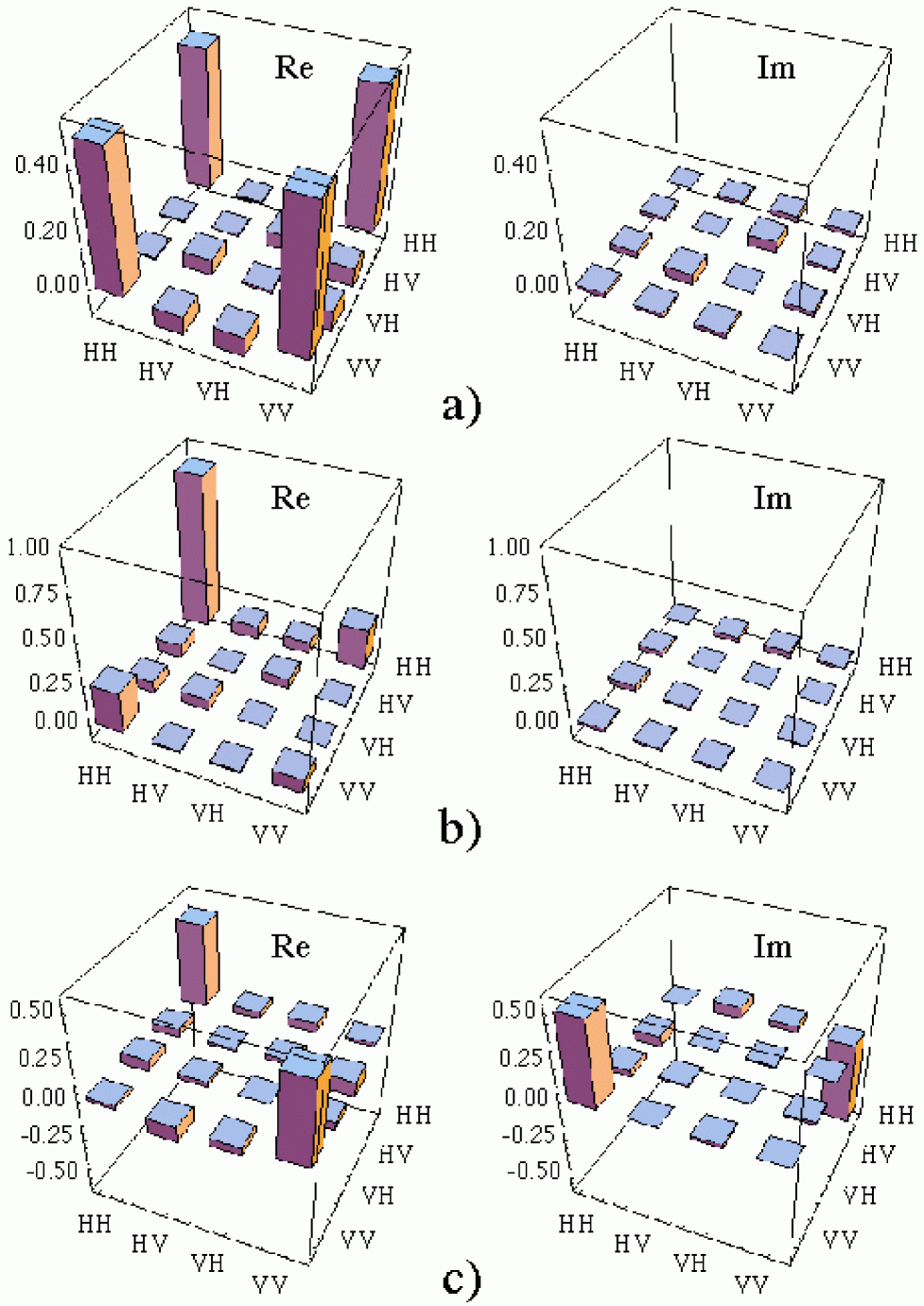
FIG. 3.: Experimentally reconstructed density matrices of states that are nominally: a) $|\rm{H}\rm{H}\rangle+|\rm{V}\rm{V}\rangle$; b) $|\rm{H}\rm{H}\rangle+0.3|\rm{V}\rm{V}\rangle$; and c) $|\rm{H}\rm{H}\rangle-i|\rm{V}\rm{V}\rangle$.

Tomography characterizes variation both in the degree of entanglement, $\varepsilon$ (compare Fig. 3b with Fig. 3a), which is set by rotating the input polarization (with UV HWP); and in the phase of entanglement, $\phi$ (compare Fig. 3c with Fig. 3a), set by tilting the input waveplate (UV QWP). Consider the maximally entangled case, Fig. 3a.

Nominally, the state is $(|\rm{HH}\rangle+|\rm{VV}\rangle)/\sqrt{2}$ - if this were true all elements, except the real corner elements, would be zero. However, as can be seen in the figure, some of the other elements are populated. What does this population signify? From the visibilities of various coincidence fringes, we know the state purity is high (the visibility is 97.8$\pm$0.1%), and further, mixture appears as real diagonal elements, so these other elements are not due to state impurity. (Unlike the single photon case, it is not possible to uniquely decompose the density matrix into pure and mixed submatrices to gain a direct measure of the state purity [30]). Instead, the $\sim$1% probability of measuring $|\rm{HV}\rangle$ and $|\rm{VH}\rangle$ terms signifies that either the axes of the analysis systems were not perfectly aligned with the axes of the source (“horizontal” at the analyzer is rotated with respect to “horizontal” at the source), or that the optic axes of the source were not perfectly orthogonal, so that the produced state is, e.g., $|\rm{HH}\rangle$+$|\rm{V^{\prime}V^{\prime}}\rangle)$, where $|\rm{V^{\prime}}\rangle\simeq|\rm{V}\rangle+\delta|\rm{H}\rangle$.

From both coincidence minima and tomography analyses, it is clear that we can controllably produce true non-maximally entangled states. As mentioned earlier, one application of such states is testing local realism. Quantum mechanics violates local realism: a quantifiable consequence of this, a statistical measure composed of coincidence measurements from a variety of analyzer settings, was first proposed by Bell [5], and has since been measured many times (see references in [15, 20]). All tests have found that, modulo some physically reasonable assumptions, nature does indeed violate local realism in accordance with quantum mechanics. At some level, however, these measurements are unsatisfying, in that the violation is at a statistical level and can only be understood after some involved logical reasoning. Recently Hardy proposed an “all-or-nothing” test of local realism [14, 15]. In brief, a state of the form $(|\rm{HH}\rangle+\varepsilon|\rm{VV}\rangle)$ is measured via four particular pairs of analyzer settings. According to any local realistic theory, if $\rm{P}_{12}(\alpha,-\alpha)=\rm{P}_{12}(\beta,-\alpha^{\perp})=\rm{P}_{12}(\alpha^{\perp},-\beta)=0$ (as can be arranged by a suitable choice of entanglement, $\varepsilon$, and analysis angles $\alpha,\beta$ [31]), then $\rm{P}_{12}(\beta,-\beta)=0$ [32]. But quantum mechanics predicts $\rm{P}_{12}(\beta,-\beta)\neq 0$. More generally, $\rm{P}_{12}(\beta,-\beta)>\rm{P}_{12}(\alpha,-\alpha)+\rm{P}_{12}(\beta,-\alpha^{\perp})+\rm{P}_{12}(\alpha^{\perp},-\beta)$, which is the inequality to be tested experimentally [16].

As Fig. 4. shows, the “Hardy-fraction”, $\rm{P}_{12}(\beta,-\beta)$, varies with degree of entanglement: for non- and maximally-entangled states the fraction is zero, so no test can be made. The data points are normalized coincidence rates measured at $\pm\beta$, (to within $0.5^{\circ}$, the inherent uncertainty in our polarization analyzers). The smooth curves are predicted directly from quantum mechanics with no adjustment parameters. Clearly there is excellent agreement. The maximum measured Hardy-fraction, $9.2$% (24222 counts), occurred at an entanglement of $\varepsilon=0.470$; the analysis angles at this point were $\alpha=55.2^{\circ}$ and $\beta=72.1^{\circ}$ - the corresponding minima

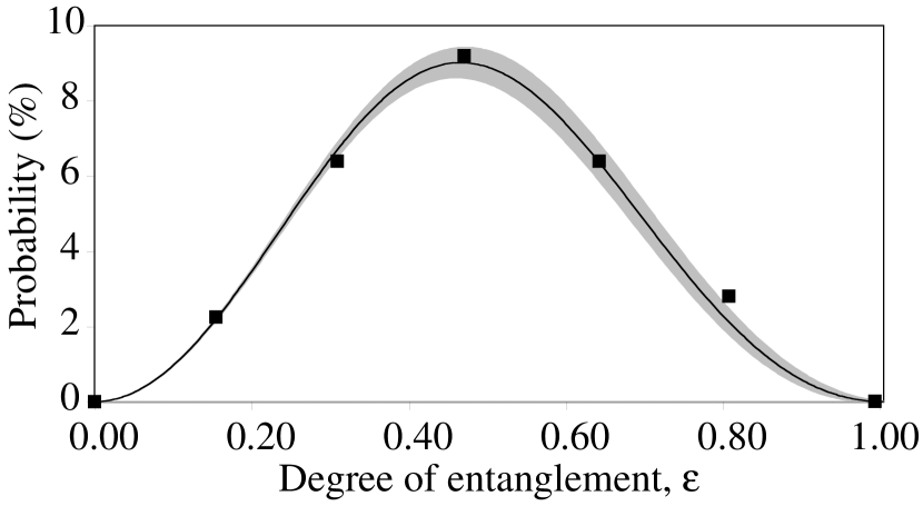
FIG. 4.: Probability of a coincidence measurement versus degree of entanglement, $\varepsilon$. points: measured probabilities obtained at $\pm(\beta\pm 0.5^{\circ})$. Uncertainties due to count statistics are small, the error bars lying within each point. curves: predictions from quantum mechanics for analysis at exactly $\pm\beta$ (black) and out to $\pm(\beta\pm 0.5^{\circ})$ (shaded area).

were $0.43$%, $0.52$%, and $0.49$% (1132, 1372, and 1279 counts, respectively). As the minima are determined experimentally the major source of error is count statistics. Combining the above values, we find that the Hardy-fraction is $122\sigma$ larger than the value allowed by any local realistic theory.

Our system should further extend access to Hilbert space, into the mixed regime, using depolarization technology described in [33], thus allowing the production and evaluation of partially-mixed states of the type $|\rm{HH}\rangle\langle\rm{HH}|+\gamma|\rm{VV}\rangle\langle\rm{VV}|$. The application of mixed states is currently an active research area in quantum information, e.g., quantum secret sharing actually requires access to mixed states in some cases [34]. Finally, we note that in principle the photons from our source are “hyper-entangled”, i.e., entangled in every degree of freedom, not just polarization [35]. Development of a tomographic technique to measure the corresponding full density matrix remains a considerable challenge.

In conclusion, we have demonstrated the production, characterization, and utilization of true non-maximally entangled quantum states, without the need for postselection. This includes a tomographic technique that measures the reduced density matrix for polarization entangled photon pairs, and a demonstration of local realism violation, which requires non-maximal entanglement.

We wish to thank Devang Naik for assistance, and Ulf Leonhardt, Bill Munro, and Mike Raymer for encouraging discussions.

REFERENCES

- [1] E. Schrödinger, Proc. Camb. Phil. Soc. 31, 555 (1935).
- [2] R. J. C. Spreeuw, Found. Phys. 28, 361 (1998).
- [3] N. J. Cerf et al., Phys. Rev. A 57, R1477 (1998); P. G. Kwiat et al., J. Mod. Opt., to appear (1999).
- [4] A. Einstein et al., Phys. Rev. A 47, 777 (1935).
- [5] J. S. Bell, Physics 1, 195 (1964).
- [6] Special issue of the Proc. Royal Soc. London, Series A-Math, Phys. & Eng. Sci., 454 (#1969) (1998).
- [7] A. K. Ekert, Phys. Rev. Lett. 67, 661 (1991).
- [8] C. Bennett and S. J. Wiesner, Phys. Rev. Lett. 69, 2881 (1992); K. Mattle et al., Phys. Rev. Lett. 76, 4656 (1996).
- [9] C. Bennett et al., Phys. Rev. Lett. 70, 1895 (1993); D. Bouwmeester et al., Nature 390, 575 (1997); D. Boschi et al., Phys. Rev. Lett. 80, 1121 (1998).
- [10] P. Hariharan and B. Sanders, Prog. in Opt. 36, 49 (1996).
- [11] Not be confused with the entropy of entanglement [C. H. Bennett et al., Phys. Rev. A 54, 3824 (1996)], which in this case is, . For , is a maximum;, for , .
- [12] J. J. Sakurai, Modern Quantum Mechanics (Addison-Wesley, Massachusetts, 2nd Edition, 1994).
- [13] P. H. Eberhard, Phys. Rev. A 47, R747 (1993); A. Garuccio, Phys. Rev. A 52, 2535 (1995).
- [14] L. Hardy, Phys. Rev. Lett. 71, 1665 (1993).
- [15] P. G. Kwiat and L. Hardy, Am. J. Phys., to appear (1999)
- [16] Any experimental realization still requires inequalities, as measurements always have uncertainties.
- [17] Q. A. Turchette et al., Phys. Rev. Lett. 81, 3631 (1998).
- [18] J. R. Torgerson et al., Phys. Lett. A 204, 323 (1995).
- [19] G. Digiuseppe et al.,, Phys. Rev. A 56, 176 (1997).
- [20] P. G. Kwiat et al., Phys. Rev. A., 60, R773 (1999).
- [21] In practice, there is a slight deviation from this relationship as the pump beam power at the second crystal is slightly attenuated due to absorption in the first crystal.
- [22] M. Born and E. Wolf, Principles of Optics (Cambridge University Press, Cambridge, 7th Edition, 1999).
- [23] D. T. Smithey et al., Phys. Rev. Lett. 70, 1244 (1993).
- [24] D. Leibfried et al., Phys. Rev. Lett. 77, 4281 (1996).
- [25] U. Leonhardt, Phys. Rev. Lett. 74, 4101 (1995).
- [26] G. G. Stokes, Trans. Camb. Phil. Soc. 9, 399 (1852).
- [27] This is the reduced density matrix, the full density matrix contains information about every degree of freedom.
- [28] Two parameters describe any position on the surface of the Poincaré sphere, i.e., definitely polarized light (a pure state); a third parameter is required to describe any position within the sphere volume, i.e., partially polarized light (a partially-mixed state). The center of the sphere represents unpolarized light (a maximally-mixed state).
- [29] These contain the normalization constants, and so are fundamentally different from the deviation density matrices in liquid NMR experiments [e.g., I. L. Chuang et al., Nature, 393, 143 (1998)], which represent the small component (typically 10-5) that deviates from the maximally-mixed state.
- [30] The density matrix can be uniquely written as , where and N is the Hilbert space dimension. However, this does not identify the mixed state fraction.
- [31] The Hardy angles are given by (where ) and .
- [32] Consider only photons that would pass a analysis, and ask what results are possible in a local realistic model if a different analysis were performed instead. These photons must pass and analyses, since . Therefore, in a local realistic model, photon 1 (2) is definitely polarized at (), and so would definitely pass an analysis. But by assumption, so .
- [33] P. D. D. Schwindt et al., Phys. Rev. A., to appear (1999).
- [34] R. Cleve et al., Phys. Rev. Lett. 82, 648 (1999).
- [35] P. G. Kwiat, J. Mod. Opt. 44, 2173 (1997).