Variational Ansatz for ${\cal PT}$-Symmetric Quantum Mechanics

Abstract

A variational calculation of the energy levels of the class of ${\cal PT}$-invariant quantum mechanical models described by the non-Hermitian Hamiltonian $H=p^{2}-(ix)^{N}$ with $N$ positive and $x$ complex is presented. The energy levels are determined by finding the stationary points of the functional $\langle H\rangle(a,b,c)\equiv\left(\int_{C}dx\,\psi(x)H\psi(x)\right)/\left(\int_{C}dx\,\psi^{2}(x)\right)$, where $\psi(x)=(ix)^{c}\exp\left(a(ix)^{b}\right)$ is a three-parameter class of ${\cal PT}$-invariant trial wave functions. The integration contour $C$ used to define $\langle H\rangle(a,b,c)$ lies inside a wedge in the complex-$x$ plane in which the wave function falls off exponentially at infinity. Rather than having a local minimum the functional has a saddle point in the three-parameter $(a,b,c)$-space. At this saddle point the numerical prediction for the ground-state energy is extremely accurate for a wide range of $N$. The methods of supersymmetric quantum mechanics are used to determine approximate wave functions and energy eigenvalues of the excited states of this class of non-Hermitian Hamiltonians.

I Introduction

In a recent letter [1] the spectra of the class of non-Hermitian ${\cal PT}$-symmetric Hamiltonians of the form

$$H=p^{2}-(ix)^{N}\quad(N\geq 2)$$ (1)

were shown to be real and positive. It has been conjectured that the reality and positivity of the spectra are a consequence of ${\cal PT}$ symmetry.

The Schrödinger differential equation corresponding to the eigenvalue problem $H\psi=E\psi$ is

$$-\psi^{\prime\prime}(x)-(ix)^{N}\psi(x)=E\psi(x).$$ (2)

To obtain real eigenvalues from this equation it is necessary to define the boundary conditions properly. This was done in Ref. [1] by analytically continuing in the parameter $N$ away from the harmonic oscillator value $N=2$. This analytic continuation defines the boundary conditions in the complex-$x$ plane. The regions in the cut complex-$x$ plane in which $\psi(x)$ vanishes exponentially as $|x|\to\infty$ are wedges. The wedges for $N>2$ were chosen to be the continuations of the wedges for the harmonic oscillator, which are centered about the negative and positive real axes and have angular opening ${\pi\over 2}$. For arbitrary $N>2$ the anti-Stokes’ lines at the centers of the left and right wedges lie below the real axis at the angles

$$\theta_{left} = -\pi+\left({N-2\over N+2}\right){\pi\over 2},$$ (3)

$$\theta_{right} = -\left({N-2\over N+2}\right){\pi\over 2}.$$ (4)

The opening angle of these wedges is ${2\pi\over N+2}$. In Ref. [1] the time-independent Schrödinger equation was integrated numerically inside the wedge to determine the eigenvalues to high precision. Observe that as $N$ increases from its harmonic oscillator value ($N=2$), the wedges bounding the integration path undergo a continuous deformation as a function of $N$.

In this work we show that the ground-state energy for the ${\cal PT}$-invariant quantum mechanical models in Eq. (1) can be obtained from the condition that the functional

$$E(a,b,c,\ldots)=\langle H\rangle(a,b,c)\equiv{\int_{C}dx\,\psi(x)H\psi(x)\over\int_{C}dx\,\psi^{2}(x)},$$ (5)

be stationary as a function of the variational parameters $a,~{}b,~{}c,~{}\ldots$ of the trial ground-state wave function $\psi(x)$. In Eq. (5) the integration contour $C$ lies in appropriate wedges in the complex plane, as explained in Sec. II.

We obtain variational approximations to the higher eigenvalues and wave functions using the following procedure [2, 3]: First, we obtain a ${\cal PT}$-symmetric superpotential from the approximate ground-state trial wave function. From this we construct a supersymmetric ${\cal PT}$-symmetric partner potential. Next, we use variational methods to find the ground-state energy and wave function of the Hamiltonian associated with the partner potential and, from that, a second superpotential. Iterating this process, we determine the higher-energy eigenvalues and the associated excited states of the original Hamiltonian.

We now review this procedure in more detail. Let us consider the Hamiltonian $H^{(0)}$ whose eigenvalues $E_{n}^{(0)}$ and eigenfunctions $\psi_{n}^{(0)}$ are labeled by the index $n$. Subtracting the ground-state energy $E_{0}^{(0)}$ from the Hamiltonian $H^{(0)}$ gives a new Hamiltonian $H^{(1)}\equiv H^{(0)}-E_{0}^{(0)}$. The eigenvalues of this new Hamiltonian are shifted accordingly, $E_{n}^{(1)}=E_{n}^{(0)}-E_{0}^{(0)}$, but the eigenfunctions of $H^{(1)}$ remain unchanged: $\psi_{n}^{(1)}(x)=\psi_{n}^{(0)}(x)$.

By construction, $H^{(1)}$ has zero ground-state energy. Thus, we may regard $H^{(1)}$ as the first component of a two-component supersymmetric ${\cal PT}$-symmetric Hamiltonian that can be written in factored form [4]:

$$H^{(1)} = A_{-}^{(1)}A_{+}^{(1)}$$ (6)

$$= [{1\over i}{d\over dx}-W^{(1)}(x)][{1\over i}{d\over dx}+W^{(1)}(x)].$$ (7)

The ground-state wave function of $H^{(1)}$ satisfies the first-order differential equation

$$[{1\over i}{d\over dx}+W^{(1)}(x)]\Psi_{0}^{(1)}(x)=0.$$ (8)

From this equation we determine the superpotential $W^{(1)}$:

$$W^{(1)}(x)=-{{\Psi_{0}^{(1)}}^{\prime}(x)\over i\Psi_{0}^{(1)}(x)}=-{{\Psi_{0}^{(0)}}^{\prime}(x)\over i\Psi_{0}^{(0)}(x)}.$$ (9)

The supersymmetric partner of $H^{(1)}$, which we call $H^{(2)}$, is given by the product of the operators $A_{\pm}^{(1)}$ in the opposite order from that in Eq. (7):

$$H^{(2)} = A_{+}^{(1)}A_{-}^{(1)}$$ (10)

$$= -{d^{2}\over dx^{2}}-\left[W^{(1)}(x)\right]^{2}-{1\over i}\left[W^{(1)}(x)\right]^{\prime}.$$ (11)

Note that the spectrum of $H^{(2)}$ is the same as the spectrum of $H^{(1)}$ except that it lacks a state corresponding to the ground state of $H^{(1)}$. It is easy to verify that the eigenstates of $H^{(2)}$ are explicitly given by $\psi_{n}^{(2)}=A_{+}^{(1)}\psi_{n+1}^{(1)}$ and the corresponding eigenvalues are $E_{n}^{(2)}=E_{n+1}^{(1)}$. Thus, if we can find the ground-state wave function and energy of $H^{(2)}$, then we can use these quantities to express the first excited wave function and energy of $H^{(0)}$:

$$\psi_{1}^{(0)}(x) = {A_{-}^{(1)}\psi_{0}^{(2)}(x)\over E_{0}^{(2)}},$$ (12)

$$E_{1}^{(0)} = E_{0}^{(2)}+E_{0}^{(0)}.$$ (13)

By iterating this procedure we can construct a hierarchy of Hamiltonians $H^{(m)}$ ($m=1,~{}2,~{}3,~{}\ldots$). The successive energy levels of $H^{(0)}$ are then obtained by finding the ground-state wave functions and energies of $H^{(2m)}$ using variational methods that we develop in Sec. II. It is important to realize that because the higher wave functions of $H^{(0)}$ require an increasing number of derivatives, we need increasingly accurate ground-state wave functions to obtain a reasonable approximation to the higher eigenvalues. A more extensive discussion of this procedure can be found in Refs. [2, 3].

This paper is organized very simply. In Sec. II we use variational methods to calculate the ground-state energy and wave function of the Hamiltonian $H$ in Eq. (1) for various values of $N$. Then in Sec. III we calculate the first few excited energy levels and wave functions. In Sec. IV we make some concluding remarks and suggest some areas for future investigation.

II Variational Ansatz for ${\cal PT}$-Symmetric Hamiltonians

In previous variational calculations [3] two-parameter “post-Gaussian” nodeless trial wave functions of the general form

$$\psi(x)=\exp\left(-a|x|^{b}\right)$$ (14)

were used to obtain estimates for the ground states of the hierarchy of Hamiltonians constructed from the anharmonic oscillator $p^{2}+x^{4}$. In this paper we obtain estimates for the ground states of the hierarchy of ${\cal PT}$-symmetric Hamiltonians arising from $H$ in Eq. (1).

The concept of ${\cal PT}$ symmetry is discussed in detail in Refs. [1] and [5]. To be precise, a function $F(x)$ of a complex argument $x$ is ${\cal PT}$ symmetric if

$$[F(x)]^{*}=F(-x^{*}).$$ (15)

Thus, any real function of $ix$ is manifestly ${\cal PT}$ symmetric. In previous numerical calculations [1] it was found that the eigenfunctions of the ${\cal PT}$-symmetric Hamiltonians in Eq. (1) were all ${\cal PT}$ symmetric. Thus, for our variational calculation we choose a three-parameter trial wave function that is explicitly ${\cal PT}$ symmetric:

$$\psi(x)=(ix)^{c}\exp\left(a(ix)^{b}\right),$$ (16)

where the variational parameters $a$, $b$, and $c$ are real.

The most notable difference between the Hermitian trial wave function in Eq. (14) and the ${\cal PT}$-symmetric trial wave function in Eq. (16) is the number of variational parameters. It is not advantageous to have a prefactor in Eq. (14) of the form $|x|^{c}$ because the expectation value of the kinetic term $-d^{2}/dx^{2}$ of the Hamiltonian does not exist unless $c>{1\over 2}$. Because of the singularity at $x=0$ we must exclude the case $c\leq{1\over 2}$ in conventional variational calculations. However, positive values of $c$ are in conflict with the large-$|x|$ behavior of the WKB approximation to the exact wave function; WKB theory predicts a negative value for the parameter $c$.

We emphasize strongly that in conventional variational calculations the integration path is the real axis. For the case of $\psi(x)$ in Eq. (14) one cannot deform the contour of integration to avoid the origin because the function $|x|$ is not analytic. More generally, the notion of path independence is not applicable in conventional variational calculus because the functional to be minimized involves an integral over the absolute square $\psi^{*}(x)\psi(x)$ of the trial wave function. For the case of ${\cal PT}$-symmetric quantum mechanics the trial wave function $\psi(x)$ in Eq. (16) is analytic in the cut $x$ plane. (The cut is taken to run along the positive-imaginary axis; this choice is required by ${\cal PT}$ symmetry.) Moreover, the functional involves an integral over the square, not the absolute square, of the wave function [5]. These two properties imply that the integration contour can be deformed so long as the endpoints of the contour lie inside of the wedge in Eq. (4). In particular, the contour may be chosen to avoid the infinite singularity at the origin that occurs when the parameter $c$ in Eq. (16) is negative. Thus, in ${\cal PT}$-symmetric quantum mechanics we can include the additional parameter $c$ anticipating that we will obtain highly accurate numerical results for the energy levels.

In general, for Hermitian Hamiltonians it is well known that the variational method always gives an upper bound for the ground-state energy. That is, the stationary point of the expectation value of the Hamiltonian in the normalized trial wave function [see Eq. (5)] is an absolute minimum. By contrast, for ${\cal PT}$-invariant quantum mechanics, too little is known about the state space to prove any theorems about the nature of stationary points. Thus, we will simply look for all stationary points of the function $E(a,b,c)$ in Eq. (5), and not just minima.

The first step in our calculation is to evaluate the functional $E(a,b,c)$ in Eq. (5). To do this we must make a definite choice of contour $C$. It is convenient to choose the path of integration in the complex-$x$ plane to follow the rays for which the trial wave function in Eq. (16) does not oscillate and falls off exponentially as $\exp\left(-ar^{b}\right)$. (We assume implicitly here that $a$ is positive.) These rays are symmetrically placed about the negative-imaginary axis. Specifically, we set

$$z=re^{i\theta_{L}},~{}~{}{\rm where}~{}~{}\theta_{L}=-{\pi\over 2}-{\pi\over b}$$ (17)

on the left side of the imaginary axis, with the path running from $r=-\infty$ to $r=0$ ($\theta_{L}$ fixed), and

$$z=re^{i\theta_{R}},~{}~{}{\rm where}~{}~{}\theta_{R}=-{\pi\over 2}+{\pi\over b}$$ (18)

on the right side of the imaginary axis, with the path running from $r=0$ to $r=\infty$ ($\theta_{R}$ fixed). Note that when $b=2$, the path lies on the real axis; for $b\neq 2$, the path develops an elbow at the origin.

Our key assumption is that this integration path lie inside the asymptotic wedges described in Eq. (4). This requirement restricts the value of $b$:

$${1\over 3}(N+2)\leq b\leq N+2.$$ (19)

Now, we evaluate the integral in Eq. (5) in terms of Gamma functions:

$$E(\alpha,\beta,\gamma) = {(\beta-\beta^{2}-\gamma)\Gamma(1-\beta-\gamma)\alpha^{2\beta}\over 4\beta^{2}\Gamma(1+\beta-\gamma)}$$ (21)

$$\qquad-{\Gamma(1-\beta-\gamma)\alpha^{-N\beta}\over\Gamma(1-\beta-N\beta-\gamma)},$$

where

$$\alpha=2a,\quad\beta=1/b,\quad\gamma=2c/b.$$ (22)

To find a stationary point of the function $E(\alpha,\beta,\gamma)$ we must calculate its partial derivatives with respect to the parameters $\alpha$, $\beta$, and $\gamma$, and determine the values of these parameters for which the partial derivatives vanish. It is simplest to calculate the derivative with respect to $\alpha$; requiring that this derivative be zero gives an expression for $\alpha$ in terms of $\beta$ and $\gamma$:

$$\alpha^{(2+N)\beta}={2N\beta^{2}\Gamma(1+\beta-\gamma)\over(\beta^{2}-\beta+\gamma)\Gamma(1-\beta-N\beta-\gamma)}.$$ (23)

Recalling that the parameter $a$, and therefore $\alpha$, must be positive gives regions in the $(\beta,\gamma)$ plane of the allowable values of $\beta$ and $\gamma$. These regions are shown as shaded areas in Fig. 1.

There are many distinct regions for which $\alpha$ is positive. We describe the boundaries of these regions in detail. First, all of these regions must satisfy the inequality

$${1\over N+2}\leq\beta\leq{3\over N+2},$$ (24)

which follows from Eq. (19). These bounds are shown as two heavy vertical lines in Fig. 1.

Second, there is an inverted parabola

$$\gamma=\beta-\beta^{2}.$$ (25)

The lowest region is bounded above by this parabola and the next higher region is bounded below by this parabola.

Third, there is an infinite sequence of downward-sloping straight lines of the general form

$$\gamma=k-\beta(N+1)\qquad(k=1,~{}2,~{}3,~{}\ldots).$$ (26)

These lines bound the shaded regions on the left and on the right.

Fourth, there is an infinite sequence of upward-sloping straight lines of the general form

$$\gamma=k+\beta\qquad(k=1,~{}2,~{}3,~{}\ldots).$$ (27)

These lines are upper and lower bounds of the shaded regions.

WKB theory predicts that

$$\alpha={4\over N+2},\quad\beta={2\over N+2},\quad\gamma=-{N\over N+2}.$$ (28)

The special WKB values $(\beta={2\over N+2},\gamma=-{N\over N+2})$ are indicated by a heavy dot in Fig. 1. Note that this point lies on the boundary of the only shaded region that lies below the $\beta$ axis. We will restrict our attention to the stationary point (there is only one) of $E(\alpha,\beta,\gamma)$ that lies in this special region because it is nearest to the WKB point. We will see that the stationary point in this special region is a local maximum as a function of $\beta$ and $\gamma$, and not a local minimum as in the case of conventional Hermitian theories.

To locate the stationary point in the $(\beta,\gamma)$ plane we solve Eq. (23) for $\alpha$ and substitute the result back into the energy functional $E(\alpha,\beta,\gamma)$ in Eq. (21). We then construct a highly-accurate contour plot of the resulting function of $\beta$ and $\gamma$. From our analysis we are able to locate the stationary points to four significant digits for various values of $N$. Our results for $N=3$, $N=4$, and $N=5$ are shown in Tables I and II. In Table III we show that in the $(\beta,\gamma)$ plane, the stationary point is a local maximum.

To verify the accuracy of the ground-state trial wave function we have calculated the normalized expectation value of $x^{P}$ using $\psi(x)$ in Eq. (16):

$${\langle 0|~{}x^{P}~{}|0\rangle\over\langle 0|0\rangle} = {\int_{C}dx\,x^{P}\psi^{2}(x)\over\int_{C}dx\,\psi^{2}(x)}$$ (29)

$$= (-i)^{P}{\Gamma(1-\beta-\gamma)\alpha^{-P\beta}\over\Gamma(1-\beta-P\beta-\gamma)}.$$ (30)

Substituting the values of $\alpha$, $\beta$, and $\gamma$ taken from Table I for $N=3$, $N=4$, and $N=5$ we display in Table IV the expectation values of $x^{P}$ for $P=1,~{}2,~{}\ldots,~{}5$. To measure the accuracy of our variational wave function we can check the numbers in Table IV in two ways. First, we have calculated the exact values of $\langle 0|~{}x~{}|0\rangle/\langle 0|0\rangle$ for $N=3$, $N=4$, and $N=5$. The values are $-0.590073i$, $-0.866858i$, and $-1.013102i$, respectively. These numbers differ from those in the first row in Table IV by about one part in a thousand. Second, combining the operator equation of motion obtained from $H$ in Eq. (1),

$$x^{\prime\prime}(t)=2iN(ix)^{N-1},$$ (31)

with the time-translation invariance of $\langle 0|~{}x~{}|0\rangle$, we find that the expectation value of $x^{N-1}$ vanishes for an $(ix)^{N}$ theory. This is evident to a high degree of accuracy in Table IV.

One further check of the accuracy of the trial wave function is to compare its asymptotic behavior with that of the WKB approximation to $\psi(x)$. For example, from Eq. (28) the WKB value of $\beta$ for $N=3$ is $0.4$. For a simpler two-parameter trial wave function in which we set $\gamma=0$, the stationary point occurs at $\beta=0.36$. For the three-parameter case we get $\beta=0.3855$, which is much closer to the value $0.4$. Indeed, all of the values in Table I are very close to the WKB values in Eq. (28).

III Higher Energy Levels

We follow the procedure outlined in Sec. I and use trial wave functions of the form in Eq. (16) to construct the first few excited states. As one might have expected, the numerical accuracy decreases for the higher states. The ground-state values of $(\alpha,\beta,\gamma)$ for the case $N=3$ are $(0.72066,0.3855,-0.157)$, as shown in Table I. For the first excited state we obtain the values $(0.55750,0.3568,-0.329)$ and for the second excited state we obtain $(0.39925,0.3255,-0.466)$. Using these parameters we predict that the first excited energy level $E_{1}$ is $4.11738$ and that the second excited energy level $E_{2}$ is $7.53886$. The exact values of $E_{1}$ and $E_{2}$ obtained by numerical integration of the Schrödinger equation (2) (see Ref. [1]) are $4.1092$ and $7.5621$. Thus, the relative errors in our calculation of $E_{0}$, $E_{1}$, and $E_{2}$ are roughly 1 part in 2000, 4 parts in 2000, and 7 parts in 2000.

For the case $N=4$ the ground-state values of $(\alpha,\beta,\gamma)$ are $(0.5800,0.3185,-0.2745)$ (see Table I). For the first excited state we obtain $(0.41763,0.2915,-0.614)$. From these parameters we predict that the first excited energy level $E_{1}$ is $6.03769$. The exact value of $E_{1}$ is $6.0033$. Thus, the relative error in this calculation of $E_{0}$ and $E_{1}$ is roughly 3 parts in 5000 and 25 parts in 5000.

TABLE I.: Variational calculation of the ground-state energy for the ${\cal PT}$-symmetric Hamiltonian in Eq. (1) for three values of $N$. The stationary point of $E(\alpha,\beta,\gamma)$ for the three-parameter trial wave function in Eq. (16) is given for $N=3$, $N=4$, and $N=5$.

$N$	$\alpha$	$\beta$	$\gamma$
3	$0.7207$	$0.3855$	$-0.1570$
4	$0.5800$	$0.3185$	$-0.2745$
5	$0.4895$	$0.2720$	$-0.3610$

TABLE II.: Variational calculation of the ground-state energy for the ${\cal PT}$-symmetric Hamiltonian in Eq. (1) for three values of $N$. Using the stationary point of $E(\alpha,\beta,\gamma)$ taken from Table I we calculate the variational value of the ground-state energy $E_{\rm var}$ and compare it with the exact value $E_{\rm exact}$ obtained by direct numerical integration of the Schrödinger equation in (2). Note that the relative error for $N=3$, $N=4$, and $N=5$ is approximately one part in $2000$.

$N$	$E_{\rm var}$	$E_{\rm exact}$	$rel.error$
3	$1.156754$	$1.156267$	$0.042\%$
4	$1.478023$	$1.477149$	$0.062\%$
5	$1.909382$	$1.908265$	$0.059\%$

TABLE III.: The stationary point of $E[\alpha(\beta,\gamma),\beta,\gamma]$ is a local maximum in the $(\beta,\gamma)$ plane. To verify this the value of $E$ for $N=4$ is given at the stationary point $\beta=0.3185$, $\gamma=-0.2745$ and at four nearby points. In a conventional Hermitian theory the stationary point would be a local minimum.

$\beta$	$\gamma$	$E(\alpha,\beta,\gamma)$
$0.3185$	$-0.2745$	$1.478023$
$0.3185$	$-0.2750$	$1.478022$
$0.3185$	$-0.2740$	$1.478022$
$0.3186$	$-0.2745$	$1.478022$
$0.3184$	$-0.2745$	$1.478022$

TABLE IV.: Normalized expectation values of $x^{P}$ in the ground state. These expectation values were calculated from the trial wave function $\psi(x)$ in Eq. (16) with $\alpha$, $\beta$, and $\gamma$ given in Table I for $N=3$, $N=4$, and $N=5$.

$P$	${\langle 0|~{}x^{P}~{}|0\rangle\over\langle 0|0\rangle}\bigm{|}_{N=3}$	${\langle 0|~{}x^{P}~{}|0\rangle\over\langle 0|0\rangle}\bigm{|}_{N=4}$	${\langle 0|~{}x^{P}~{}|0\rangle\over\langle 0|0\rangle}\bigm{|}_{N=5}$
1	$-0.590686i$	$-0.867264i$	$-1.013266i$
2	$-0.000767$	$-0.518220$	$-0.864749$
3	$-0.462705i$	$0.000869i$	$0.518217i$
4	$-0.385363$	$-0.492631$	$0.002080$
5	$-0.363227i$	$0.635997i$	$0.545538i$

Having verified that the variational calculation of the energies of the excited states is extremely accurate, we turn to the wave functions. We have performed two tests of the accuracy of the variational wave functions. First, we have computed the integral of the square of the wave functions. In general, we expect that the integral of the square of the $n$th excited wave function to be a real number having the sign pattern $(-1)^{n}$. This is precisely what we find for the $N=3$ wave functions ($\psi_{0}$, $\psi_{1}$, and $\psi_{2}$) and the $N=4$ wave functions ($\psi_{0}$ and $\psi_{1}$) that we have studied. To understand the origin of this alternating sign pattern recall the form of the wave functions for the harmonic oscillator [the $N=2$ case of Eq. (1)]. The harmonic oscillator is ${\cal PT}$ symmetric and all of its eigenfunctions can be made ${\cal PT}$ symmetric upon multiplying by the appropriate factor of $i$. The first three eigenfunctions in explicit ${\cal PT}$-symmetric form are, apart from a real multiplicative constant,

$$\psi_{0}(x) = e^{(ix)^{2}/2},$$ (32)

$$\psi_{1}(x) = (ix)e^{(ix)^{2}/2},$$ (33)

$$\psi_{2}(x) = [2(ix)^{2}+1]e^{(ix)^{2}/2}.$$ (34)

These wave functions exhibit precisely this $(-1)^{n}$ behavior.

Second, we have found the nodes of the variational wave functions. For $N=3$ the ground-state variational wave function is nodeless and the first excited state variational wave function has one node at $x=-0.703i$. These results are extremely accurate: The exact ground-state wave function is also nodeless and the exact first-excited-state wave function has one node at $x=-0.533i$. We observe the same qualitative features for the case $N=4$; here, the node of the first excited state, as determined by our variational calculation, is located at $x=-0.972i$.

IV Conclusions

The results of this investigation suggest several intriguing avenues of research. The most surprising aspect of this variational calculation is that even though the stationary point is a saddle point in parameter space, and not a minimum, this saddle point clearly gives correct physical information. Clearly, it is the nonpositivity of the norm that accounts for the fact that the stationary point is a saddle point. The norm used in this paper is

$$\int_{C}dx\,\psi^{2}(x)$$ (35)

rather than the conventional choice

$$\int_{C}dx\,\psi^{*}(x)\psi(x).$$ (36)

However, the accuracy of the variational approach suggests that we have found an extremely powerful technique for obtaining approximate solutions to complex Sturm-Liouville eigenvalue problems.

A possible explanation for the accuracy of our approach is that while the norm we are using is not positive definite in coordinate space, we believe that it is positive definite in momentum space. The positivity for our choice of norm is easy to verify in the special case of the harmonic oscillator. We believe that this positivity property does not undergo a sudden transition as we analytically continue the theory into the complex plane by increasing $N$. We point out that the strong advantage of our choice of norm is that $\psi^{2}(x)$ is an analytic function while $\psi^{*}(x)\psi(x)$ is not. This allows us to analytically continue Sturm-Liouville problems into the complex plane. (We point out that until now, Sturm-Liouville problems have been limited to the real axis.)

An extremely interesting question to be considered in the future is the completeness of the eigenfunctions of a complex ${\cal PT}$-symmetric Sturm-Liouville problem. It is easy to show that the eigenfunctions corresponding to different eigenvalues are orthogonal:

$$\int_{C}dx\,\psi_{m}(x)\psi_{n}(x)=0\quad(m\neq n).$$ (37)

However, it is not known whether the eigenfunctions form a complete set and what norm should be used in this context. It is clear that in order to answer questions regarding completeness, a full understanding of the distribution of zeros of the wave functions must be achieved. For a Sturm-Liouville problem limited to the real axis completeness depends on the zeros becoming dense. For the case of a regular Sturm-Liouville problem the zeros interlace as they become dense. Our preliminary numerical investigations suggest that the zeros of the eigenfunctions of complex ${\cal PT}$-symmetric Sturm-Liouville problems also become dense in the complex plane and exhibit a two-dimensional generalization of the interlacing phenomenon.

One area that we have investigated in great detail is the extension of these quantum mechanical variational calculations to quantum field theory [6]. The natural technique to use is based on the Schwinger-Dyson equations; successive truncation of these equations is in exact analogy with enlarging the space of parameters in the trial wave functions. We find that the Schwinger-Dyson equations provide an extremely accurate approximation scheme for calculating the Green’s functions and masses of a ${\cal PT}$-symmetric quantum field theory.

Finally, we remark that the notion of probability in quantum mechanics is connected with the positivity of the norm in Sturm-Liouville problems. We note that the conventional quantum mechanical norm is neither an analytic function nor invariant with respect to ${\cal PT}$ symmetry, while the momentum-space version of the norm in Eq. (35) is both. It would be a remarkable advance if one could formulate a fully ${\cal PT}$-symmetric quantum mechanics.

We thank Dr. S. Boettcher for assistance in doing computer calculations. This work was supported in part by the U.S. Department of Energy.

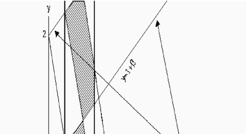
FIG. 1.: Regions (shown as shaded) of acceptable values of $\beta$ and $\gamma$. These values of $\beta$ and $\gamma$ are acceptable because they give positive $\alpha$ in Eq. (23).

REFERENCES

- [1] C. M. Bender and S. Boettcher, Phys. Rev. Lett. 80, 5243 (1998).
- [2] E. Gozzi, M. Reuter and W. Thacker, Phys. Lett. A 183, 29 (1993); F. Cooper, J. Dawson and H. Shepard, Phys. Lett. A 187, 140 (1994).
- [3] F. Cooper, A. Khare, U. Sukhatme, Phys. Reports 251, 267 (1995).
- [4] The conventional product decomposition of the Hamiltonian used in Refs. 2 and 3 has the form . However, such a factorization does not respect symmetry; in order to maintain symmetry it is necessary for each to be accompanied by a factor of . By the factorization used in Eq. (7) we have a decomposition that is simultaneously supersymmetric and symmetric. Field theoretic Hamiltonians that are both supersymmetric and symmetric are examined in C. M. Bender and K. A. Milton, Phys. Rev. D 57, 3595 (1998).
- [5] In -symmetric quantum mechanics we use the integral of the square of the wave function rather than the integral of the absolute square of the wave function because the statement of orthogonality is if . Unlike the case of conventional quantum mechanics the orthogonality condition involves a complex integral of an analytic function and thus the integration path may be deformed. In conventional quantum mechanics the corresponding integral is restricted to the real axis and the path cannot be deformed. See C. M. Bender, S. Boettcher, and P. N. Meisinger, J. Math. Phys. 40, 2201 (1999).
- [6] C. M. Bender, K. A. Milton, and V. M. Savage, submitted.