Abstract

Suppose that we are given a quantum computer programmed ready to perform a computation if it is switched on. Counterfactual computation is a process by which the result of the computation may be learnt without actually running the computer. Such processes are possible within quantum physics and to achieve this effect, a computer embodying the possibility of running the computation must be available, even though the computation is, in fact, not run. We study the possibilities and limitations of protocols for the counterfactual computation of decision problems (where the result $r$ is either 0 or 1). If $p_{r}$ denotes the probability of learning the result $r$ “for free” in a protocol then one might hope to design a protocol which simultaneously has large $p_{0}$ and $p_{1}$. However we prove that $p_{0}+p_{1}\leq 1$ in any protocol of this type and derive further constraints on $p_{0}$ and $p_{1}$ in terms of $N$, the number of times that the computer is not run. In particular we show that any protocol with $p_{0}+p_{1}=1-\epsilon$ must have $N$ tending to infinity as $\epsilon$ tends to 0. We show that “interaction-free” measurements can be regarded as counterfactual computations, and our results then imply that $N$ must be large if the probability of interaction is to be close to zero. Finally, we consider some ways in which our formulation of counterfactual computation can be generalised.

Keywords: quantum computation,measurement, counterfactual,interaction-free

1 Introduction

There is a set of remarkable phenomena that seem to be special to quantum mechanics. Their common theme is counterfactuality: the fact that an event might have happened enables one to obtain some information about that event, even though it did not actually take place. Examples of such counterfactual phenomena include the Elitzur-Vaidman bomb testing problem (Elitzur & Vaidman 1993, Penrose 1994) and the use of so-called interaction-free measurements (Kwiat et al. 1995, Renninger 1960, Dicke 1981, Geszti 1998) to determine the presence or absence of an object by means of a test particle, even though no “interaction” may have occurred between the object and the particle. With some protocols, the probability of an interaction occurring can be made arbitrarily small. By carrying out a raster-scan of such measurements, it is possible to form an image of an object in an interaction-free manner (White et al. 1998).

One can extend these ideas and imagine the object being replaced by a quantum computer (Jozsa 1999). In that case, it turns out that one can determine the outcome of a computation without the computer ever being switched on. This is counterfactual computation. In the quantum formalism the computer may be in a superposition of being on and off, and we will need to clarify the sense in which the computer is “not switched on”. This is the content of our precise definition of counterfactual computation given below. There are many possible protocols for counterfactual computation which give various probabilities of gaining information ‘for free’. The aim of this paper is to show that there are limits on these probabilities which hold for all possible protocols; there are also limits for protocols depending on how often the computer is given the opportunity to run (in a sense to be made precise). As we shall see, counterfactual computation includes interaction-free measurement as a special case, and our limits then translate into statements about the probability of interaction.

It is well known that quantum physics has a profound bearing on issues of computation as described for example in (Bernstein & Vazirani 1993, Deutsch 1985, Deutsch & Jozsa 1992, Ekert & Jozsa 1996, Grover 1996, Simon 1994, Shor 1994). Much of that work is directed towards questions of computational complexity, in particular devising quantum algorithms that exhibit an exponential speedup over any known classical algorithm for the computational task. Counterfactual computation is a novel quantum computational effect of an entirely different sort. It does not involve a speedup but highlights in a particularly poignant way, some of the interpretational enigmas of quantum mechanics and its theory of measurement. It remains to be seen whether it can be exploited for real practical benefit.

2 Defining counterfactual computation

We begin by formalising the idea of counterfactual (henceforth abbreviated to CF) computation. Consider a quantum computer with an ‘on-off’ switch programmed ready to solve a decision problem when the switch is turned to ‘on’. This computer has an output register that represents the binary result of the computation. The switch and the output register will be denoted by a pair of qubits ${\cal S}\otimes{\cal O}$, with $\cal S$ the switch qubit and $\cal O$ the output register. The switch states ‘off’ and ‘on’ are labelled respectively as $\left|0\right\rangle$ and $\left|1\right\rangle$.

The computer will generally require extra storage qubits for its programming and extra working qubits for its computational processing. If $\cal R$ denotes the state space of these extra qubits then the total state space of the computer is ${\cal S}\otimes{\cal O}\otimes{\cal R}$. As is customary in idealised quantum computation, we will assume that the computer operates in a fully reversible manner and that the initial and final states of $\cal R$ are equal. Also the binary result $r$ of the computation is deposited in the output register qubit as an addition modulo 2. Thus the computational process may be written

$$\begin{array}[]{ll}\left|0\right\rangle\left|j\right\rangle\left|R\right\rangle\rightarrow\left|0\right\rangle\left|j\right\rangle\left|R\right\rangle&\mbox{(computer `off')}\\ \left|1\right\rangle\left|j\right\rangle\left|R\right\rangle\rightarrow\left|1\right\rangle\left|j\oplus r\right\rangle\left|R\right\rangle&\mbox{(computer `on')}\end{array}$$ (1)

and it is completed in some finite known time $T$.

If the computer is switched on, after a time $T$ it will have carried out one of two unitary operations $U_{0}$ or $U_{1}$ on ${\cal S}\otimes{\cal O}$ corresponding to the two possible outputs $r=0$ or $r=1$. Here $U_{0}$ is the identity on the switch and register qubits and $U_{1}$ is the C-NOT operation on these two qubits (cf eq. (1)). Thus $U_{0}$ takes $|10\rangle$ into $|10\rangle$ and $U_{1}$ takes $|10\rangle$ into $|11\rangle$ but if the computer is not switched on then the evolution is the same for both possible values of $r$ (in fact, being then $U_{0}$).

We will assume that the computer is given as a device with the switch and output qubits ${\cal S}\otimes{\cal O}$ initially set to $\left|0\right\rangle\left|0\right\rangle$. If the switch is set to $\left|1\right\rangle$ the computer will effect either the transformation $U_{0}$ or $U_{1}$ and we wish to determine which it is, without switching it on. We will assume that we are unable to access the qubits in $\cal R$.

We begin with a row of qubits (as long as required) all initialised in a standard state $\left|0\right\rangle$. A protocol consists of a sequence of steps where each step is one of the following:
(a) A unitary operation (not involving the computer) on a finite number of specified qubits.
(b) A measurement on a finite number of specified qubits.
(c) An “insertion of the computer”, where the state of two selected qubits is swapped into the registers ${\cal S}\otimes{\cal O}$ of the computer, a time $T$ is allowed to elapse and finally the states are swapped back out into the two selected qubits.
The steps of the protocol are implemented by selecting the designated qubits from the row, applying the operation and then returning the qubits to their positions in the row. The whole protocol may be thought of as a network of operations with the computer being inserted at various places via (c). The same $U_{r}$ is used throughout the protocol. The outcomes of the measurements in (b) are the source of our information about the computation and its result.

To understand how a protocol works and to provide a definition of counterfactual computation, we introduce a notation which records whether the computer was on or off on the various occasions when it was inserted. At the beginning of any such step the entire state space can be partitioned into two orthogonal subspaces, the ‘off’ and ‘on’ subspaces, corresponding to the switch states $|0\rangle$ and $|1\rangle$, respectively, and we will separate the total state into its two superposition components in these subspaces.

Imagine that, after each insertion of the computer, we carried out a measurement that projects into these subspaces, with outcomes which we write compactly as $f$ (for off) or $n$ (for on). Then each possible list of $f/n$ outcomes, together with outcomes of the measurements in the protocol, defines what we shall call a history. One can depict this imaginary protocol as a branching structure. At each node we give the un-normalised state vector, the result of the projections occurring at each measurement step of the protocol or at the imaginary measurement following an insertion of the computer. If $v_{n}$ denotes the un-normalised state vector at the final node of the history $h$, the probability of $h$ is $|v_{h}|^{2}$. The initial node is assumed to correspond to the specified initial state of the row of qubits. Note that there will be a different branching structure depending on whether $U_{0}$ or $U_{1}$ is being used.

In the real protocol, we do not necessarily carry out the $f/n$ measurement (though of course a protocol could include such a measurement). Thus in contrast to actual measurement steps of type (b), the unnormalised state vectors at the $f/n$ branchings still retain the information of relative phases between them i.e. the branching gives two coherent superposition components of the state vector. Then we can utilise the branching structure of the imaginary protocol to compute probabilities for the real protocol as follows. Let $m$ denote a sequence of measurement outcomes, one for each measurement step of type (b) in the protocol. There will be various histories $h$ that include those outcomes (we write $m\subset h$). For instance, in Example 1 below, with $U_{0}$ the histories $f0f00$ and $n0f00$ both include the measurement outcomes $m=0,00$. (Here the first measurement in the protocol is of one qubit, giving the ‘0’, whereas the second measurement is of two qubits, giving ‘00’; see Figure 1). The probability of $m$ is just $|\sum_{m\subset h}v_{h}|^{2}$, the sum being taken over all histories including $m$. The contributions from these histories parameterised by $f/n$ sequences, are added coherently as the $f/n$ branchings do not correspond to actual measurements. (If an $f/n$ measurement is actually performed, its designated outcome will be listed in $m$ instead).

Note that our use of the term ‘history’ differs from the more conventional use (e.g. in the so-called consistent histories approach to quantum mechanics). In the latter, every node is viewed as a measurement and different paths (histories) are always added incoherently (i.e. as a sum of squares rather than a square of a sum) in computing the probability of a sequence $m$ of specified outcomes of a subset of all the measurements performed.

We are now ready to define a CF computation. Let $m$ denote a sequence of measurement outcomes. We say that $m$ is a CF outcome of type $r$, where $r=0$ or $1$, if a history $h$ including $m$ satisfies $v_{h}\neq 0$ with $U_{r}$ only if $h$ is all-off, and if the probability of $m$ with $U_{1-r}$ is zero. This means that if we observe the measurement sequence $m$ then we can infer that the computation result is certainly $r$ even though the computer has not run at any stage of the protocol (since $m$ can only occur via an all-off history). More formally we have:

Definition: $m$ is a CF outcome of type $r$, where $r=0$ or 1, if
1) With $U_{r}$, $v_{h}=0$ for all $h$ with $m\subset h$, except for that $h$ that has only $f$’s (in addition to $m$).
2) With $U_{1-r}$, $\sum_{h,m\subset h}v_{h}=0$, the sum being over all $h$ that include the measurement outcomes $m$; i.e. with $U_{1-r}$, $m$ is seen with probability zero.

Let us pause to elaborate on the sense in which “the computer has not been run at any stage” if the CF outcome sequence $m$ is observed. The reader may object that the computer has certainly been in a superposition of ‘off’ and ‘on’ and in this sense, has actually been run! But the sequence $m$ can arise only via all-off histories so if it is seen then we have been confined to a part of the total quantum state in which the computer is never run. For example, in the language of the many worlds interpretation, we will have evolved in a world in which the computer was never run yet in that world we learn the result of the computation. The fact that the computer may have run in another world is of no consequence for us. The validity of this point is especially emphasised in the original Elitzur-Vaidman bomb testing problem (Elitzur & Vaidman 1993) (which we will later see as a special case of our CF formalism): there is always a world in which a good bomb will explode but (with a suitable measurement outcome) we are confined to another world in which the bomb is left unexploded and yet we have the knowledge that it is, in fact, a good bomb, available for future explosive applications.

This issue is at the heart of the so-called measurement problem of quantum theory. Consider the proverbial Schrödinger cat in state $\frac{1}{\sqrt{2}}(\left|\rm alive\right\rangle+\left|\rm dead\right\rangle)$. What happens upon a measurement of alive versus dead? Suppose that the outcome is seen to be “alive”. Then in the conventional “collapse of wavefunction” formalism, the state of the cat changes discontinuously into $\left|\rm alive\right\rangle$ and the $\left|\rm dead\right\rangle$ component ceases to have any further physical reality or existence or any further consequence. In a many-worlds or decoherence view (Zurek 1991) of the measurement process both components $\left|\rm alive\right\rangle$ and $\left|\rm dead\right\rangle$ persist and may be thought of as existing in separate “parallel” worlds. The measurer similarly passes into all these parallel worlds, registering respectively all possible measurement outcomes. Since $\left|\rm alive\right\rangle$ and $\left|\rm dead\right\rangle$ are macroscopically distinct states they rapidly interact with many other subsystems in the external universe, spreading orthogonality. This process is the decoherence of the initial superposition which we symbolically write as:

$$\begin{array}[]{lll}\left|\rm dead\right\rangle\left|0\right\rangle\left|0\right\rangle\ldots\left|0\right\rangle&\rightarrow&\left|\rm dead\right\rangle\left|0\right\rangle\left|0\right\rangle\ldots\left|0\right\rangle\\ \left|\rm alive\right\rangle\left|0\right\rangle\left|0\right\rangle\ldots\left|0\right\rangle&\rightarrow&\left|\rm alive\right\rangle\left|1\right\rangle\left|1\right\rangle\ldots\left|1\right\rangle\end{array}$$ (2)

Here $\left|0\right\rangle$ and $\left|1\right\rangle$ are orthogonal states and the (very long) string of kets after the leftmost ket represent a large number of subsystems in the universe. Hence the two worlds or branches will never again interfere in practice – re-interference would require an enormous correlated effect to undo the widespread interaction in eq. (2) and is extremely improbable. Hence although the cat exists dead in the other world, we in this world (having perceived the outcome “alive”) will never have to bother about or suffer any consequences of that other unfortunate outcome. In either interpretation we would be happy that the cat continues to exist fully alive, despite that fact that it was in a strange superposition in the past.

In a similar way in our definition of CF outcome, the desirable option (like cat alive) is the computer being off and the undesirable option (like cat dead) is the computer being on. Although we pass through a superposition of these states, the observation of a CF outcome means either that we have collapsed the state to an entirely “off” part of the total state and the “on” part ceases to have any further physical reality or consequences, or that we are in a world in which the computer has not run, yet in both cases we also have the result of the computation.

We note also that neither of the interpretations of the measurement problem described above is really satisfactory: in the first, no mechanism is given for the discontinuous “collapse” of the state and in the second, no explanation is given of why we actually perceive just one of the parallel worlds upon making a measurement – it is difficult to present tangible physical evidence for the existence of the other worlds.

Example 1

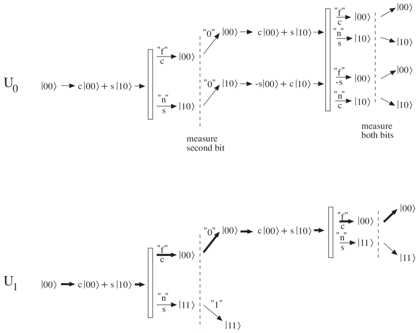
Figure 1: The protocol for Example 1, for the case $N=2$, shown as a branching structure, as described in the text. The thin boxes denote insertions of the computer and the dotted vertical lines measurements. Here $c=\cos\theta$ and $s=\sin\theta$. Arrows are labelled by $f$ or $n$, and by measurement outcomes (these are all shown in inverted commas). The sequence of labels defines the history associated to a path. For instance, the uppermost path with $U_{1}$, marked with heavy arrows, is the history $f0f00$. At each node the un-normalised state vector is shown. Under $U_{1}$, this is the only history including the measurement outcomes $m=0\mbox{ and }00$, and it is an all-$f$ history, so condition 1) for a CF outcome of type 1 is satisfied. Under $U_{0}$ there are two histories including $m$, namely $f0f00$ and $n0f00$, and the sum of their final un-normalised state vectors is $(c^{2}-s^{2})\left|00\right\rangle$. If we chose $\theta=\pi/4$ so $c^{2}-s^{2}=0$, the probability of $m$ under $U_{0}$ is zero, so condition 2) for a CF outcome is satisfied.

The following example is given in (Jozsa 1999) but we re-express it here in terms of our formalism. The only variables that concern us are the switch and output register qubits. Starting with $|00\rangle$, the state is rotated to $\cos\theta|00\rangle+\sin\theta|10\rangle$, where $\theta=\frac{\pi}{2N}$ for some integer $N$. A time $T$ is then allowed for the computer to run, if it is going to. This gives the state $\cos\theta|00\rangle+\sin\theta|1r\rangle$, assuming $U_{r}$ is used ($r=0$, $1$). The second qubit is now measured. If $r=1$, the measurement either gives $|00\rangle$ with probability $\cos^{2}\theta$, or $|11\rangle$ with probability $\sin^{2}\theta$. If the latter occurs, we know that $r=1$ and the computer has run; the protocol therefore halts. If $r=0$ the measurement yields $\cos\theta|00\rangle+\sin\theta|10\rangle$, and we repeat the preceding steps, rotating by $\theta$, allowing the machine to run, then measuring. The branching structures for $U_{0}$ and $U_{1}$ are shown in Figure 1.

After $N$ repeats, if $r=0$ the state will have rotated to $|10\rangle$ with certainty. If $r=1$, the state will be $|00\rangle$ with probability $\cos(\pi/2N)^{2N}$. In this case the computer has not run, yet we know that $r=1$. This is therefore an example of a CF computation. (In Figure 1, the history that gives the CF result is shown by bold arrows.) By making $N$ large enough, $\cos(\pi/2N)^{2N}$ can be brought arbitrarily close to 1. Thus if $r=1$ we obtain the CF result with a probability approaching 1.

Example 2

We describe next a protocol where both types of CF outcome occur (see Figure 2). In addition to the switch and output qubits, we require a third, ancillary, qubit. To start with, the initial state $|000\rangle$ is rotated to $c|000\rangle+s|100\rangle$, where $c=\cos\theta$, $s=\sin\theta$. Next we insert the computer on the first two qubits and finally measure all qubits in the following basis:

$|x_{1}\rangle=t(s|000\rangle-c|100\rangle+s|001\rangle)$,
$|x_{2}\rangle=t(s|000\rangle-c|110\rangle-s|001\rangle)$,
$|x_{3}\rangle=u(c|000\rangle+2s|100\rangle+c|001\rangle)$,
$|x_{4}\rangle=u(c|000\rangle+2s|110\rangle-c|001\rangle)$,
$|x_{5}\rangle=|010\rangle$, $|x_{6}\rangle=|101\rangle$,
$|x_{7}\rangle=|011\rangle$, $|x_{8}\rangle=|111\rangle$,

where $t=1/\sqrt{1+s^{2}}$, $u=1/\sqrt{2+2s^{2}}$. There are two CF outcomes, $\left|x_{1}\right\rangle$ with $r=1$ and $\left|x_{2}\right\rangle$ with $r=0$. They satisfy our two conditions, namely: 1) the history leading to $\left|x_{1}\right\rangle$ under $U_{1}$ has only ‘f’s, as does that leading to $\left|x_{2}\right\rangle$ under $U_{0}$, and 2) $\left|x_{1}\right\rangle$ has probability zero under $U_{0}$ as does $\left|x_{2}\right\rangle$ under $U_{1}$. The probabilities of these CF outcomes are both $(cst)^{2}$. This is maximised by $c^{2}=2-\sqrt{2}$ which gives $(cst)^{2}=0.172$, or $p_{0}+p_{1}=0.344$.

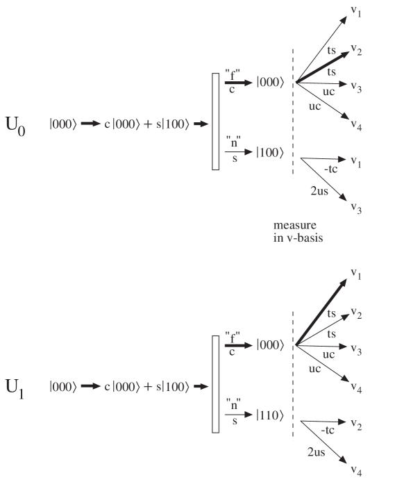
Figure 2: The protocol for Example 2. Here the first two qubits are, as usual, the switch and output register, and the third qubit corresponds to an ancilla. The only vectors in the $x$-basis relative which have non-zero probability of being final outcomes are those shown in the figure. The bold arrows show the histories that give CF outcomes; there is one of type 0 and one of type 1.

3 Limits on counterfactual computation

Let us write $p_{0}$, $p_{1}$ for the probabilities of getting a CF outcome of type 0 or type 1, respectively in any given protocol. Example 1 shows that there is a protocol for which $p_{1}$ approaches 1, but in this case $p_{0}=0$. Could one devise a protocol that allowed both $p_{0}$ and $p_{1}$ to approach 1? Less ambitiously, can one devise a protocol giving $p_{0}+p_{1}>1$? These questions were posed in Jozsa (1999), and we answer them here.

First note that, since the subdivision into on-off subspaces corresponds to an orthogonal decomposition of the entire state space (and the same is true of each measurement step of type (b)), we have, for each $U_{r}$

$$\sum_{h}|v_{h}|^{2}=1.$$ (3)

In Figure 1, for instance, under $U_{0}$ we have $\sum_{h}|v_{h}|^{2}=c^{4}+c^{2}s^{2}+s^{4}+c^{2}s^{2}=1$, for any $\theta$. This is true despite the fact that the final states of the histories may not be orthogonal for the original protocol e.g. $c^{2}\left|00\right\rangle$ and $-s^{2}\left|00\right\rangle$ for $U_{0}$ in figure 1; we are using the fact that each step in the histories is either a measurement in the protocol, or can be regarded as one (as in our imaginary protocol).

This basic fact may be alternatively expressed as follows. We imagine a supply of extra qubits, as many of them as there are insertions of the computer in our protocol. If we carry out a C-NOT operation between the switch qubit and the $n$-th extra qubit at the $n$-th insertion, the resultant states at each branching of the imaginary protocol will be mutually orthogonal in the extended space. Hence the branching tree corresponds to a probabilistic process, and eq. (3) expresses the certainty of following some path through the tree.

Now we know from condition 1) above that the all-off history $h$ alone determines the probability $|v_{h}|^{2}$ of the CF outcome. But, for an all-off history $h$, $v_{h}$ must be the same whether $U_{0}$ or $U_{1}$ is used, since the computer is never switched on! Thus, in forming the sum $p_{0}+p_{1}$, i.e. in collecting terms $|v_{h}|^{2}$ for all possible CF outcomes, one can assume that all of these terms come from the list of $v_{h}$’s for one of the $U_{r}$, say $U_{0}$. Note that condition 1) implies that there is no possible overlap: one can only get a CF outcome with one of the $U_{r}$ for a given $m$.

Thus $p_{0}+p_{1}=\sum_{h\in\cal F}|v_{h}|^{2}$, where the sum is over the set $\cal F$ of all-off terms from CF outcomes. These terms can be assumed to be derived using $U_{0}$, so equation (3) implies:

Theorem 3.1. $p_{0}+p_{1}\leq 1$.

This answers the conjecture in Jozsa (1999). We now look at some subsidiary questions.

In Example 1, one can only approach the bound of 1 closely by having a large number, $N$, of insertions of the computer. Could there be protocols which reach the bound of 1, or come close, with only a few insertions? The following argument shows that this is not possible.

Consider first the situation shown in Table 1. There is only one CF outcome, and we ask how many insertions of the computer we need to get the probability of this result, $p_{1}$, to satisfy $p_{1}=1-\epsilon$.

Table 1: One CF outcome, $M_{1}$.

	$U_{0}$	$U_{1}$
$M_{1}$	0	off only
$M_{2}$	x	x
..	..	..

Let $h(i)$ denote a history consistent with measurement outcome sequence $M_{i}$. Under $U_{0}$ we have:

$$\sum_{h(1)}|v_{h(1)}|^{2}=1-\sum_{h(i),i\geq 2}|v_{h(i)}|^{2}\leq 1.$$

Let $F(1)$ denote the all-$f$ history consistent with $M_{1}$. Then

$$p_{1}=|v_{F(1)}|^{2}\leq 1-\sum_{h(1)\neq F(1)}|v_{h(1)}|^{2},$$

so,

$$\sum_{h(1)\neq F(1)}|v_{h(1)}|^{2}\leq\epsilon.$$ (4)

On the other hand the total un-normalised state vector (under $U_{0}$ still) for $M_{1}$ is zero, so

$$\sum_{h(1)}v_{h(1)}=0.$$ (5)

Thus

$$\sum_{h(1)\neq F(1)}v_{h(1)}=-v_{F(1)},$$ (6)

and hence

$$\left|\sum_{h(1)\neq F(1)}v_{h(1)}\right|^{2}=|v_{F(1)}|^{2}=1-\epsilon.$$ (7)

Now, for any vectors $x_{i}$, the minimum of $\sum_{i=1}^{K}|x_{i}|^{2}$ given $|\sum_{i=1}^{K}x_{i}|^{2}=S$ is $S/K$. There are $2^{N}$ histories consistent with $M_{1}$ for $N$ computer insertions, so

$$\sum_{h(1)\neq F(1)}|v_{h(1)}|^{2}\geq(1-\epsilon)2^{-N}.$$

Using equation (4), $(1-\epsilon)2^{-N}\leq\epsilon$, or

$$N\geq\log_{2}\left(\frac{1-\epsilon}{\epsilon}\right).$$ (8)

Table 2: Both CF outcomes: $r=1$ ($M_{1}$) and $r=0$ ($M_{2}$).

	$U_{0}$	$U_{1}$
$M_{1}$	0	off only
$M_{2}$	off only	0
$M_{3}$	x	x
..	..	..

Consider next the situation shown in Table 2. Here both types of counterfactual result occur, and we assume $p_{0}+p_{1}=1-\epsilon$. Under $U_{0}$ we have

$$|v_{F(1)}|^{2}+|v_{F(2)}|^{2}+\sum_{h(1)\neq F(1)}|v_{h(1)}|^{2}\leq 1.$$

Since $p_{0}=|v_{F(1)}|^{2}$ and $p_{1}=|v_{F(2)}|^{2}$, we obtain (4) as before. Furthermore, equations (5) and (6) hold, but now the equivalent of (7) is

$$\left|\sum_{h(1)\neq F(1)}v_{h(1)}\right|^{2}=|v_{F(1)}|^{2}=p_{1}.$$ (9)

We therefore obtain, in place of (8), $N\geq\log(p_{1}/\epsilon)$. On the other hand, under $U_{1}$ we have $N\geq\log(p_{0}/\epsilon)$. Since $\max(p_{0},p_{1})\geq(1-\epsilon)/2$ we conclude that

$$N\geq\log_{2}\left(\frac{1-\epsilon}{2\epsilon}\right).$$ (10)

In Tables 1 and 2 only one CF outcome of each type is shown. However, no real extra generality is gained by allowing several CF outcomes of the same type. To see this, note that in each measurement step of type (b), instead of collapsing the state, we may leave it entangled with an auxiliary system representing the measurement pointer. Thus each measurement step becomes a unitary operation of type (a). Finally at the end of the protocol we read all of the pointers together. This may be viewed as a single measurement whose possible outcomes are the possible measurement sequences of the original protocol. All CF outcomes of one type can then be grouped into a single final measurement outcome.

We summarise these results as follows:

Theorem 3.2. The number of insertions $N$ must tend to infinity as $p_{0}+p_{1}$ tends to 1.

It is possible that the inequalities (8) and (10) can be sharpened. This is certainly true when $N=1$. Consider first the situation where only one type of CF outcome occurs (Table 1). The only possible histories are $fi$ or $ni$, where $i$ denotes outcome $M_{i}$. With $U_{0}$, (3) gives

$$\sum_{i}|v_{fi}|^{2}+|v_{ni}|^{2}=1.$$

Since $v_{f1}+v_{n1}=0$ we have

$$2|v_{f1}|^{2}=1-\sum_{i>=2}\left(|v_{fi}|^{2}+|v_{ni}|^{2}\right).$$ (11)

We can also add the un-normalised state vectors leading to $M_{1}$, $M_{2}$, etc, and consider just the projections onto the subspaces of the final measurement. This gives:

$$\sum_{i>=2}|v_{fi}+v_{ni}|^{2}=1,$$ (12)

where the sum goes from $i=2$ because $v_{f1}+v_{n1}=0$. From equations (11) and (12) we get

$$p_{1}=|v_{f1}|^{2}=1/4-1/2\sum_{i>=2}|v_{fi}-v_{ni}|^{2}\leq\frac{1}{4}.$$ (13)

For $N=1$, (8) implies $\epsilon\geq 1/3$, or $p_{1}\leq 2/3$, so (13) is an improvement; in fact, (13) is best possible because Example 1 with $N=1$ gives $p_{1}=1/4$. (More precisely we would need an extra final rotation step, omitted from figure 1, at the end of the protocol before measuring both bits.)

Consider next the case where both types of CF outcome occur (Table 2). With $U_{0}$, (3) gives

$$\sum_{i}|v_{fi}|^{2}+|v_{ni}|^{2}=1.$$

and now $v_{f1}+v_{n1}=0$ and $v_{n2}=0$, so

$$2|v_{f1}|^{2}+|v_{f2}|^{2}=1-\sum_{i>=3}\left(|v_{fi}|^{2}+|v_{ni}|^{2}\right).$$ (14)

Again, we can add the un-normalised state vectors leading to $M_{1}$, $M_{2}$, etc, which gives:

$$|v_{f2}|^{2}=1-\sum_{i>=3}|v_{fi}+v_{ni}|^{2},$$ (15)

Equations (14) and (15) imply

$$4|v_{f1}|^{2}+|v_{f2}|^{2}=1-\sum_{i>=3}|v_{fi}-v_{ni}|^{2}.$$

With $U_{1}$ we get

$$|v_{f1}|^{2}+4|v_{f2}|^{2}=1-\sum_{i>=3}|v_{fi}-\tilde{v}_{ni}|^{2}.$$

the tilde in $\tilde{v}_{ni}$ distinguishing the state vector with $U_{1}$ from that with $U_{0}$. Adding the last two equations gives:

$$5|v_{f1}|^{2}+5|v_{f2}|^{2}=2-(\mbox{positive terms}),$$

so

$$p_{0}+p_{1}\leq 2/5.$$ (16)

For $N=1$, (10) implies $\epsilon\geq 1/5$, or $p_{0}+p_{1}\leq 4/5$, so (16) is an improvement. We do not know, however, whether it is best possible. In Example 2, $p_{0}+p_{1}=0.344$. Can we attain the bound of (16) with some other protocol?

4 ‘Interaction-free’ measurements

Our formalisation of counterfactual computation provides a general framework that includes ‘interaction-free’ measurements (IFM) (Elitzur & Vaidman 1993, White et al. 1998, Vaidman 1996) as a special case which is characterised as follows. Suppose we have an apparatus and an object. We interpret the switch qubit as defining configurations in which the apparatus cannot interact with the object (switch=$\left|0\right\rangle$), or can (switch=$\left|1\right\rangle$), and we interpret the output register qubit as defining the state of the object, with $\left|0\right\rangle$ signifying ‘no interaction’ and $\left|1\right\rangle$ ‘interaction has occurred’. The additional constraint that defines an IFM is that each insertion of the computer, now viewed as a potential interaction between apparatus and object, is followed by a measurement of the output register. If this is $\left|1\right\rangle$, an interaction has occurred and the protocol halts. In contrast, in a general CF protocol, the output register may be set to $\left|1\right\rangle$ also by other unitary steps (not involving the computer) and the $\left|1\right\rangle$ branches may be used in subsequent interferences.

In an IFM protocol we interpret $U_{0}$ as the computation corresponding to the object being absent, and $U_{1}$ to that when it is present. Thus $p_{1}$ is the probability of an IFM occurring. As for $p_{0}$, it can be interpreted as the probability of the system being confined to the non-interactive configuration when the object is absent. This is a rather artificial concept, and theorem 3.1 does not translate into a very meaningful result. More interesting is the implication of theorem 3.2:

Theorem 4.1. The number of times $N$ an interaction with an object does not occur must tend to infinity as the probability of an IFM tends to 1.

Our Example 1 can be interpreted as an IFM, since the output register is measured after every insertion. Example 2 cannot be so interpreted, however, since the measurement following the insertion leaves the output register in a superposition of the states $\left|0\right\rangle$ and $\left|1\right\rangle$.

5 More general CF computation

Our definition of CF computation may be generalised in various natural ways such as the following. We may be given more than two unitary operations $U_{r}$ on a product space ${\cal S}\otimes{\cal O}$, whose parts may be larger than just qubits. Each operation $U_{r}$ is required to have and “on” and “off” subspace defined by an orthogonal partition of $\cal S$ and $U_{r}$ is the identity on its “off” subspace. Given an unknown one of the $U_{r}$’s we wish to determine $r$ while being confined to its “off” subspace.

We now describe an explicit example of this type of generalisation which allows the switch space $\cal S$ to have an arbitrary number of dimensions, and which also allows more than two operations $U_{r}$, but $\cal O$ is still taken to be a qubit. We consider later in more detail the case where there are only two $U_{r}$’s but an arbitrary dimensional switch space, and prove an analogue of theorem 3.2.

Our example is motivated by thinking of an interferometer in which the incoming photon is split into an equal superposition of $K$ arms, numbered 0 to $K-1$, with absorbing objects blocking all the arms except for arm 0 and arm $r$ ($r\neq 0$). The problem is to identify the value of $r$ without an interaction occurring. Our protocol below will also be an IFM in the sense of section 4 i.e. the protocol measures the output register after each potential interaction and halts if an interaction is seen to have occurred. However this IFM problem differs from standard IFM, where no prior assumption is made about the object being present or absent; here we consider a special set of configurations of objects.

More formally we consider a $K$ dimensional switch with state space $\cal S$ spanned by $\{\left|0\right\rangle,\ldots,\left|K-1\right\rangle\}$. The output register $\cal O$ is still a qubit and we define $K-1$ unitary operators $U_{r}$ for $r=1,\ldots,K-1$ on ${\cal S}\otimes{\cal O}$ by:

$U_{r}(\left|ij\right\rangle)=\left|ij\right\rangle$, if $i=0,r$ (the ‘off’-subspace),
$U_{r}(\left|ij\right\rangle)=\left|i,1-j\right\rangle$, if $i\neq 0,r$ (the ‘on’-subspace).

Thus $U_{r}$ corresponds to arms 0 and $r$ being unblocked. The “off” subspace for $U_{r}$ (on which $U_{r}$ is the identity) is ${\rm span}(\left|0\right\rangle,\left|r\right\rangle)\otimes{\cal O}$ while the “on” subspace (on which $U_{r}$ negates the output qubit value) is the orthogonal complement. Given an unknown one of the $U_{r}$’s we wish to identify $r$ while confining ourselves to its “off” subspace. More formally we modify our original definition of CF outcome as follows:

Definition: $m$ is a CF outcome of type $r$ if
1) With $U_{r}$, $v_{h}=0$ for all $h$ with $m\subset h$, except for that $h$ that has only $f$’s.
2) With $U_{s}$, $s\neq r$, $m$ is seen with probability zero.

Consider now the following protocol. Starting with $\left|00\right\rangle$, we apply to the switch a unitary transformation $R$ given by

$$R(\left|00\right\rangle)=a\left|00\right\rangle+\sum_{i=1}^{K-1}b\left|i0\right\rangle,$$

and

$$R(\left|j0\right\rangle)=-b\left|00\right\rangle+\left|j0\right\rangle+\sum_{i=1}^{K-1}\frac{(a-1)}{(K-1)}\left|i0\right\rangle,j\neq 0.$$

where $a^{2}+(K-1)b^{2}=1$. We now insert $U_{r}$, then measure the output register. If it is $\left|1\right\rangle$ the protocol terminates; otherwise the protocol continues by repeating the above. After $\pi/2b$ steps the protocol halts. We may show (cf the geometric interpretation of the process below) that as $b$ decreases, the probability of interaction occurring decreases. In a way that is similar to example 1, for small enough $Kb$ the final state is, with high probability, $\left|r0\right\rangle$. According to our definition above, this will then be a CF outcome of type $r$.

The workings of the protocol may be understood in terms of a geometrical interpretation of its operations. Consider first the case $K=3$. Looking at the switch variable, $R$ is just a rotation in the plane of $\left|0\right\rangle$ and $\left|1\right\rangle+\left|2\right\rangle$, i.e. about the axis $\left|1\right\rangle-\left|2\right\rangle$ which is orthogonal to those two states. To see this just note that $R$ is some rotation (as columns are orthonormal and det$(R)=1$) and $R$ leaves $\left|1\right\rangle-\left|2\right\rangle$ fixed. The angle of rotation is given by $\cos\theta=\langle v|Rv\rangle$ for any choice of $v$ in the rotation plane; taking $v=\left|0\right\rangle$ gives $\cos\theta=a$. The protocol can then be thought of as follows: $R$ repeatedly applied gradually pushes the state $\left|0\right\rangle$ around to the equal superposition of all the other basis states, except that after each incremental rotation $R$, the state is projected into the 2D space of $\left|0\right\rangle$ and $\left|r\right\rangle$ (so long as the output register is always measured to be $\left|0\right\rangle$). It is clear that $\left|0\right\rangle$ will be pushed around to $\left|r\right\rangle$ and we get $p_{r}$ near $1$ for all $r$’s if $b$ is sufficiently small, keeping the state always close to the rotation plane. This 2D motion is not a simple rotation because of the repeated projections (which do not commute with $R$). If the output register is ever measured to be $\left|1\right\rangle$, the state has been projected orthogonal to the rotation space and we abort the process.

For general $K$ the operation $R$ on the switch variable is just the same rotation in the 2D subspace of $\left|0\right\rangle$ and $\left|1\right\rangle+\left|2\right\rangle+\ldots\left|K-1\right\rangle$, being the identity in the orthogonal $(K-2)$-dimensional complement $C$. To see this note that $R$ leaves invariant all $K-2$ vectors of the form $\left|1\right\rangle-\left|r\right\rangle$, $r=2,\ldots,K-1$. These vectors are all orthogonal to both $\left|0\right\rangle$ and $\left|1\right\rangle+\left|2\right\rangle+\ldots\left|K-1\right\rangle$ so they span $C$. The angle of rotation is as given above and again we get a 2D motion in the plane of $\left|0\right\rangle$ and $\left|r\right\rangle$.

Now consider $K=3$ again: As in our original definition of CF computation, there are two operations, here $U_{1}$ and $U_{2}$, but now the switch variable’s dimension is three (i.e. the switch is a “qutrit”). Both $p_{1}$ and $p_{2}$ have a natural interpretation, (the probability of an IFM if an object is in arm 2 or 1, respectively), so one might hope that theorem 3.1 would yield a meaningful result. However, the theorem (stating that $p_{1}+p_{2}\leq 1$) evidently fails in this generalised setting since both $p_{1}$ and $p_{2}$ tend to 1 for small enough $b$. The reason for this failure is that the proof assumes that the two $U_{r}$’s have the same ‘off’ subspace. This was true of the original $U_{r}$’s but is not true in the present case as the switch qutrit is $\left|0\right\rangle$ or $\left|1\right\rangle$ in the ‘off’ space of $U_{1}$, and is $\left|0\right\rangle$ or $\left|2\right\rangle$ in the ‘off’ space of $U_{2}$. We therefore cannot hope to prove an equivalent of theorem 3.1. However, we show next that a version of theorem 3.2 does hold, namely that the number of steps must be large for $p_{0}+p_{1}$ to approach its upper bound. This bound is 2 in the present example rather than 1.

This new theorem holds not only for IFMs, but for any CF computations, given certain restrictions on the ‘on’- and ‘off’-subspaces of the $U_{r}$’s. We label the two $U_{r}$’s as $U_{0}$ and $U_{1}$ again, but now allow any finite dimensional switch space ${\cal S}$. We assume that $\cal S$ is partitioned into orthogonal ‘on’- and ‘off’-subspaces for each of $U_{0}$ and $U_{1}$, and we also assume that these decompositions are compatible in the sense that the subspaces

${\cal S}_{a}$= [$U_{0}$ ‘off’ & $U_{1}$ ‘on’],
${\cal S}_{b}$= [$U_{0}$ ‘on’ & $U_{1}$ ‘off’],
${\cal S}_{f}$= [$U_{0}$ ‘off’ & $U_{1}$ ‘off’],
${\cal S}_{n}$= [$U_{0}$ ‘on’ & $U_{1}$ ‘on’],

span the whole of ${\cal S}$. We also assume that $U_{0}$ is the identity on ${\cal S}_{a}\otimes{\cal O}$ and ${\cal S}_{f}\otimes{\cal O}$, and $U_{1}$ is the identity on ${\cal S}_{b}\otimes{\cal O}$ and ${\cal S}_{f}\otimes{\cal O}$. With these assumptions we have

Theorem 5.1. The number $N$ of insertions must tend to infinity as $p_{0}+p_{1}$ tends to its maximum value.

The proof is given in the Appendix. Note that the theorem applies to the 3-armed interferometer as ${\cal S}_{a}=\{\left|1\right\rangle\}$, ${\cal S}_{b}=\{\left|2\right\rangle\}$, ${\cal S}_{f}=\{\left|0\right\rangle\}$ and ${\cal S}_{n}=\emptyset$, and these subspaces span S. Here there are two operations $U_{r}$, but it seems likely that theorem 5.1 can be generalised to any number of operations satisfying appropriate compatibility conditions on their ‘on’ and ‘off’ subspaces.

6 Discussion

Our starting point was the enticing notion of being able to run a quantum computer ‘for free’. The quotation marks here were very necessary, however, for it is not at all clear what if anything comes for free. A CF protocol requires the computer to be present, and due time must allowed for the machine not to run. If the computer does not run, then we might expect to gain protection against decoherence. However, this appears not to be the case because our computer has to eschew all dissipative processes if running it is to constitute a unitary operation (as is necessary in a CF protocol to correctly generate the destructive interferences which allow us to conclude that an outcome is CF for a value of $r$), even though it might not actually be run. Perhaps the computer owner could determine whether the machine had run and levy a charge accordingly; we would then at least make a financial gain from a CF computation. Suppose, for instance, at each step where there was an ‘on’-‘off’ choice the owner arranged for the switch state to be entangled with an extra qubit. At the end of the run he could measure the extra qubits to see what path the computation had taken. However, it is easy to see (in example 1 for instance) that this measurement generally destroys the interference that gives rise to a CF outcome.

Thus the naive notion of gain from a general CF computation has to be abandoned. It does not follow, however, that CF computation is a meaningless abstraction. As we have seen, the framework includes ‘interaction-free’ measurement, where (despite the quotation marks) the practical gain is real, since it includes such potential benefits as X-ray images with reduced radiation damage (Vaidman 1996). By making the definition of CF computation sufficiently broad, we might hope to capture other types of interesting counterfactuality. In the last section we took some steps towards generalising our initial definition. We conclude by suggesting two further steps in this direction. These are both probabilisitic extensions of CF computation.

First, suppose the output register is extended to $K+1$ values, and that running the computer takes the state $|10\rangle\otimes|x\rangle$ to $|1r\rangle\otimes|x\rangle$ under $U_{r}$, for $r=0,\ldots,K$, where $|x\rangle=|0\ldots 0\rangle$ in a $2^{K}$-dimensional ancillary Hilbert space. By analogy with Example 2, one can rotate $|00\rangle\otimes|x\rangle$ to $(c|00\rangle+s|10\rangle)\otimes|x\rangle$, insert the computer, then measure in a basis including $|v_{r}\rangle=t(s|00\rangle-c|1r\rangle)\otimes|x\rangle+ts|00\rangle\otimes|y_{r}\rangle$, where the $|y_{r}\rangle$ are vectors from the barycentre of a $K$-simplex to its vertices satisfying $\langle y_{i}|y_{j}\rangle=-1$, $|y_{i}|^{2}=K$ and $t=1/\sqrt{1+Ks^{2}}$. If we see the outcome corresponding to $|v_{s}\rangle$, we know that the output register did not take the value $s$, and also that the computer did not run. Thus we have some counterfactual information, but do not know precisely what value the output register took. However, given prior probabilities for the $U_{r}$, we can compute posterior probabilities for output $r$.

The other type of probabilistic extension is obtained by relaxing the conditions (1) and (2) in the definition of CF computation. We may define a measurement outcome sequence $m$ to be “approximately CF for $r$” if it has the following properties. For some (small) $\epsilon$:
($1^{\prime}$) With $U_{r}$, $\sum|v_{h}|^{2}<\epsilon$ where the sum is over all histories consistent with $m$ except for the all-off history (the latter history having probability significantly larger than $\epsilon$).
($2^{\prime}$) With $U_{1-r}$, $m$ is seen with probability less than $\epsilon$.
Hence if $m$ is seen then with high probability the computational result is $r$ and also with high probability, no computation has been done.
Appendix A.
We give here a proof of theorem 5.1.

Proof. The upper bound here is 2, so suppose $p_{0}+p_{1}=2-\epsilon$, for small $\epsilon>0$.

We decompose ${\cal S}\otimes{\cal O}$ into subspaces ${\cal S}_{r}\otimes{\cal O}$, where $r=a,b,f,n$, and label each component before an insertion with the appropriate subscript. Just as we previously wrote histories as chains of $f$’s and $n$’s (and measurement outcomes, which we suppress), we can now write histories as chains of $a$’s, $b$’s, $f$’s and $n$’s. We have

$$p_{0}\leq|\sum_{a,f}v_{s}|^{2},$$ (17)

where $s$ ranges over all strings composed of $a$’s and $f$’s, and $v_{s}$ is obtained under $U_{0}$. Similarly for $p_{1}$ we have,

$$p_{1}\leq|\sum_{b,f}v_{s}|^{2},$$ (18)

with $b$’s and $f$’s, under $U_{1}$.

Now consider a protocol with $N$ insertions. After the first insertion (17) and (18) imply

$p_{0}\leq|v_{a}+v_{f}|^{2}=|v_{a}|^{2}+|v_{f}|^{2}$, (under $U_{0}$)
$p_{1}\leq|v_{b}+v_{f}|^{2}=|v_{b}|^{2}+|v_{f}|^{2}$, (under $U_{1}$).

Also,

$$|v_{a}|^{2}+|v_{b}|^{2}+|v_{f}|^{2}\leq 1,$$

where the first term is derived under $U_{0}$, the second under $U_{1}$ and the third under either. This holds because the $U_{r}$ are all the identity on the subspaces in question. These inequalities imply $|v_{f}|^{2}\geq p_{0}+p_{1}-1$ and $|v_{a}|^{2}+|v_{b}|^{2}\leq 2-p_{0}-p_{1}$, which implies $|v_{a}|+|v_{b}|\leq\sqrt{4-2p_{0}-2p_{1}}$. Since $p_{0}+p_{1}=2-\epsilon$, we get

$|v_{f}|^{2}\geq 1-\epsilon$.
$|v_{a}|+|v_{b}|\leq\sqrt{2\epsilon}$.

Note that the first inequality implies ${\cal S}_{f}$ is non-empty.

Now look at the situation after n insertions. From (17) we have, under $U_{0}$:

$$p_{0}\leq|\sum_{k=0}^{k=n-2}\sum_{s}v_{f^{k}as^{n-k-1}}+v_{f^{n-1}a}+v_{f^{n}}|^{2}.$$ (19)

Here $f^{k}as^{n-k-1}$ denotes a history beginning with $k$ $f$’s, followed by an $a$, then followed by some string of $n-k-1$ a’s or $f$’s. A similar inequality holds for $p_{1}$.

We make the inductive hypothesis:

$$|v_{f^{k}a}|+|v_{f^{k}b}|\leq\delta_{k},\mbox{ for k }\leq n-1,$$

where $\delta_{k}$ can be made as small as desired by taking $\epsilon$ small enough. We have established this for $n=1$.

Applying the triangle inequality to (19), we get

$$p_{0}\leq\left[|\sum_{k=0}^{k=n-2}\sum_{s}v_{f^{k}as^{n-k-1}}|+|v_{f^{n-1}a}+v_{f^{n}}|\right]^{2},$$

and using the orthogonality of ${\cal S}_{a}$ and ${\cal S}_{f}$ and the bound $|v_{f^{n-1}a}+v_{f^{n}}|\leq 1$ we get

$$p_{0}\leq\left(\sum_{k=0,s}^{k=n-2}|v_{f^{k}as^{n-k-1}}|\right)^{2}+2\sum_{k=0,s}^{k=n-2}|v_{f^{k}as^{n-k-1}}|+|v_{f^{n-1}a}|^{2}+|v_{f^{n}}|^{2},$$

with a similar expression for $p_{1}$. Applying our inductive hypothesis gives

$$p_{0}+p_{1}\leq|v_{f^{n-1}a}|^{2}+|v_{f^{n-1}b}|^{2}+2|v_{f^{n}}|^{2}+2\sum_{k=0}^{k=n-2}u_{k}\delta_{k}+\left(\sum_{k=0}^{k=n-2}u_{k}\delta_{k}\right)^{2},$$

where $u_{k}$ counts the number of strings $s$ for $k$. If we write this as

$$|v_{f^{n-1}a}|^{2}+|v_{f^{n-1}b}|^{2}+2|v_{f^{n}}|^{2}\geq p_{0}+p_{1}-y$$

where $y$ can be made small by choosing $\epsilon$ small enough (by the inductive hypothesis), we can subtract

$$|v_{f^{n-1}a}|^{2}+|v_{f^{n-1}b}|^{2}+|v_{f^{n}}|^{2}\leq 1$$

to obtain

$$|v_{f^{n}}|^{2}\geq 1-\epsilon-y.$$ (20)

We also get

$$|v_{f^{n-1}a}|+|v_{f^{n-1}b}|\leq\sqrt{2(\epsilon+y)},$$

and putting $\delta_{n-1}=\sqrt{2(\epsilon+y)}$ establishes the inductive hypothesis.

Now we reintroduce measurement outcomes in the notation. Asumme $p_{i}$ is determined from the measurement $M_{i}$. We can write

$$p_{i}=|v_{f^{n}i}+\sum_{a,f}v_{si}|^{2},$$ (21)

for $i=$0 or 1. As we are assuming $p_{0}+p_{1}=2-\epsilon$ we have $p_{i}\geq 1-\epsilon$ for $i=$0 or 1, and hence, taking the square root in (21)

$$|v_{f^{n}i}+\sum_{a,f}v_{si}|\geq 1-\epsilon.$$

Using the triangle inequality and adding the results for $i=$0 and 1 gives

$$|v_{f^{n}0}|+|v_{f^{n}1}|+|\sum_{a,f}v_{s0}|+|\sum_{b,f}v_{s1}|\geq 2-2\epsilon.$$

As the subspaces for $M_{0}$ and $M_{1}$ are orthogonal, $|v_{f^{n}0}|^{2}+|v_{f^{n}1}|^{2}\leq 1$, implying $|v_{f^{n}0}|+|v_{f^{n}1}|\leq\sqrt{2}$. So we have

$$|\sum_{a,f}v_{s0}|+|\sum_{b,f}v_{s1}|\geq 2-\sqrt{2}-2\epsilon.$$ (22)

Eq. (3) implies $\sum_{a,f}|v_{s0}|^{2}+\sum_{b,f}|v_{s1}|^{2}+|v_{f^{n}}|^{2}\leq 1$ so from (20) we infer

$$\sum_{a,f}|v_{s0}|^{2}+\sum_{b,f}|v_{s1}|^{2}\leq\epsilon+y.$$ (23)

We now use the minimisation result that gave us theorem 3.2, namely that, for any vectors $x_{i}$, $\sum_{i=1}^{K}|x_{i}|^{2}\geq|\sum_{i=1}^{K}x_{i}|^{2}/K$. Applying this to either of the terms on the left-hand side of (22) and (23) gives $\epsilon+y\geq(2-\sqrt{2}-2\epsilon)^{2}/2^{N}$, and by choosing $\epsilon$ small enough we can ensure that $N$ must be as large as we please.

References

- [1]
- [2] Bernstein, E. and Vazirani, U. 1993 Quantum complexity theory. Proc. 25th Annual ACM Symposium on the Theory of Computing, (ACM Press, New York), pp. 11-20.
- [3]
- [4] Deutsch, D. 1985 Quantum-theory, the Church-Turing principle and the universal quantum computer. Proc. Roy. Soc. London Ser. A, vol. 400, pp. 97-117.
- [5]
- [6] Deutsch, D. and Jozsa, R. 1992 Rapid solution of problems by quantum computation. Proc. Roy. Soc. London Ser A, vol. 439, pp. 553-558.
- [7]
- [8] Dicke, R. H., Interaction-free quantum measurements – a paradox. 1981 Am. J. Phys. 49, pp. 925-930.
- [9]
- [10] Ekert, A. and Jozsa, R. 1996 Quantum computation and Shor’s factoring algorithm. Rev. Mod. Phys., vol. 68, pp. 733-753.
- [11]
- [12] Elitzur, A. C. and Vaidman, L. 1993 Quantum mechanical interaction-free measurements. Found. of Phys., vol. 23, pp. 987-997.
- [13]
- [14] Geszti, T. 1998 Interaction-free measurement and forward scattering. Phys. Rev. A, vol. 58, pp. 4206-4209.
- [15]
- [16] Grover, L. 1996 A fast quantum mechanical algorithm for database search. Proc. 28th Annual ACM Symposium on the Theory of Computing, (ACM Press, New York), pp. 212-219.
- [17]
- [18] Jozsa, R. 1999 Quantum effects in algorithms. Chaos, Solitons and Fractals, vol. 10, pp. 1657-1664. Also available at http://xxx.lanl.gov/quant-ph/9805086.
- [19]
- [20] Kwiat, P. G., Weinfurter, H., Herzog, T., Zeilinger, A. and Kasevich, M. A. 1995 “Interaction-free” measurement. Phys. Rev. Lett., vol. 74, pp. 4763-4766.
- [21]
- [22] Penrose, R. 1994 Shadows of the Mind, Oxford University Press.
- [23]
- [24] Renninger, M. 1960 Messungen ohne Stoerung des Meszobjekts. Z. Phys., vol. 158, pp. 417-420.
- [25]
- [26] Shor, P. 1994 Algorithms for quantum computation: Discrete logarithms and factoring. Proc. of 35th Annual Symposium on the Foundations of Computer Science, (IEEE Computer Society, Los Alamitos), pp. 124-134.
- [27]
- [28] Simon, D. 1994 On the power of quantum computation. Proc. of 35th Annual Symposium on the Foundations of Computer Science, (IEEE Computer Society, Los Alamitos), pp. 116-123.
- [29]
- [30] Vaidman, L. 1996 Interaction-free meaurement. Preprint available at http://xxx.lanl.gov/quant-ph/9610033.
- [31]
- [32] White, G. A., Mitchell, F. R., Nairz, O. and Kwiat, P. G. 1998 “Interaction-free” Imaging. Preprint available at http://xxx.lanl.gov/quant-ph/9803060.
- [33]
- [34] Zurek, W. H. 1991 Decoherence and the transition from quantum to classical. Physics Today, October, pp. 36-44.
- [35]