Non-Markovian dynamics in pulsed and continuous wave atom lasers

Abstract

The dynamics of atom lasers with a continuous output coupler based on two-photon Raman transitions is investigated. With the help of the time-convolutionless projection operator technique the quantum master equations for pulsed and continuous wave (cw) atom lasers are derived. In the case of the pulsed atom laser the power of the time-convolutionless projection operator technique is demonstrated through comparison with the exact solution. It is shown that in an intermediate coupling regime where the Born-Markov approximation fails the results of this algorithm agree with the exact solution. To study the dynamics of a continuous wave atom laser a pump mechanism is included in the model. Whereas the pump mechanism is treated within the Born-Markov approximation, the output coupling leads to non-Markovian effects. The solution of the master equation resulting from the time-convolutionless projection operator technique exhibits strong oscillations in the occupation number of the Bose-Einstein condensate. These oscillations are traced back to a quantum interference which is due to the non-Markovian dynamics and which decays slowly in time as a result of the dispersion relation for massive particles.

I Introduction

Nowadays it is a standard technique to produce a Bose-Einstein condensate in the laboratory [5, 6]. In order to build a coherent source of atoms, an atom laser, a major achievement was the coherent extraction of atoms from an atomic trap. At first a pulsed atom laser was built [7, 8], recently also continuous wave atom lasers have been realized [9, 10]. A short survey over the experimental situation is given in [11, 12].

The theoretical treatment of an atom laser is usually based on the Born-Markov approximation [13, 14, 15, 16, 17], which has been used in quantum optics with great success. However, as it has been shown recently by Moy and coworkers [18], this approximation fails in a realistic parameter regime. In this article we will outline a different approach, which is based on the time-convolutionless (TCL) projection operator technique [19, 20, 21] to study non-Markovian effects resulting from the output coupling. This technique is based on a perturbative expansion in powers of the output coupling strength.

The master equation resulting from the perturbative expansion has a form similar to the Born-Markov master equation and is also local in time. This makes the equation of motion easy to solve. As we will see the second order perturbation theory corresponds to the Born-Markov approximation. By taking higher orders of the expansion non-Markovian effects can be studied in a systematic way. It is demonstrated that the perturbative expansion holds in an intermediate coupling regime, which corresponds to realistic parameters, while the Born-Markov approximation fails for these parameters.

This paper consists of two parts and is structured as follows. In section II we investigate the validity of the time-convolutionless projection operator technique (TCL) for a pulsed atom laser. The model investigated was discussed by Moy et al. [18]. They showed that the Born-Markov approximation fails for realistic parameters. We demonstrate that the time-convolutionless projection operator technique agrees with the exact solution for these parameters. Afterwards we apply the TCL algorithm to a simple model of a continuous wave atom laser in section III. The numerical results obtained from a simulation using a perturbation expansion including 4th order clearly reveal strong oscillations in the occupation number of the Bose-Einstein condensate (BEC). As will be shown these oscillations can be interpreted as a quantum interference effect which clearly reveals departures from the golden rule and demonstrating the non-Markovian dynamics of the atom laser. A short summary concludes the article.

II Pulsed atom lasers

In this part we will investigate the dynamics of a pulsed atom laser. This means that there is an output coupling mechanism which transfers the atoms out of the trap but there is no pump mechanism which supplies the BEC with new atoms. When the trap is empty it is replenished and a new cycle starts. Therefore our starting point is an existing BEC inside an atomic trap and we study only the output coupling.

This part is organized as follows. We briefly introduce our atom laser model and derive the exact equation of motion for the expectation value of the atomic number operator of the BEC in section II A. In section II B we discuss the Born-Markov approximation. The TCL-algorithm is then applied to the model in section II C. Afterwards the numerical results are discussed in section II D. A model of a continuous wave atom laser which includes a pumping mechanism to compensate losses by the output coupling will be introduced in part III.

A Exact solution

Usually, the output coupling from a BEC to a large reservoir is described within the Born-Markov approximation. This description is based upon a master equation of the form

$$\frac{d}{dt}\rho_{\text{sys}}(t)=\gamma_{M}\;{\cal D}[a]\,\rho_{\text{sys}}(t)\;,$$ (1)

where the single trap mode occupied by the BEC is described by the creation and annihilation operators $a^{\dagger},a$ and $\gamma_{M}$ is the Markovian decay rate. The superoperator ${\cal D}$ is of Lindblad form [22] and is defined by

$${\cal D}[a]\,P=aPa^{\dagger}-\frac{1}{2}(a^{\dagger}aP+Pa^{\dagger}a)\;.$$ (2)

In the Markovian approach one obtains a master equation containing only system variables. Two basic assumptions underlying the Born-Markov approximation are that (i) if the system and the reservoir are uncorrelated at the beginning they remain uncorrelated for later times and (ii) that the evolution of the system is Markovian. The Markovian property means that the future evolution of the system depends only on the present state and is independent of the previous history of the system. As it is shown in Ref. [18] the Born-Markov approximation is not valid in a realistic parameter regime of atom lasers.

We want to investigate a Raman output coupler through state change, which was suggested by Moy et al. [18, 23, 24, 25]. Two lasers are tuned to a two-photon resonance to couple an initial atomic state inside the trap to a final atomic state outside the trap. Due to the conservation of linear momentum the atoms receive momentum kicks during the Raman transitions which pushes the atoms out of the trap. If we assume that the lasers are detuned far from single photon resonances, then all initially empty modes of the atomic trap remain empty and we can neglect all modes besides the ground state mode occupied from the BEC. In addition, we also ignore the effects of atom-atom interactions. The resulting Hamiltonian $H$ is of the form

$$H = H_{\text{sys}}+H_{\text{res}}+H_{\text{int}},$$ (4)

$$H_{\text{sys}} = \hbar\omega_{0}\,a^{\dagger}a,$$ (5)

$$H_{\text{res}} = \int_{-\infty}^{+\infty}dk\,\hbar\omega_{k}\;b_{k}^{\dagger}b_{k},$$ (6)

$$H_{\text{int}} = -i\hbar\,(Ba^{\dagger}-B^{\dagger}a)\;,$$ (7)

where we have defined

$$B=\int_{-\infty}^{+\infty}dk\,\kappa(k)b_{k}\;,\quad\quad\omega_{k}=\frac{\hbar k^{2}}{2M}\;.$$ (8)

The bosonic creation and annihilation operators for the free atomic state are denoted by $b_{k}^{\dagger},b_{k}$. The ground state trap energy is denoted by $\hbar\omega_{0}$ and $\hbar\omega_{k}$ is the energy of the free output atomic state, $M$ is the atomic mass. The function $\kappa(k)$ describes the strength and spectral form of the coupling. In the specific case of a Raman output coupler and a harmonic trap with a Gaussian ground state [24, 25] of width $\sigma_{k}$ in $k$-space given by

$$\Psi(k)=(2\pi\sigma_{k})^{-1/4}\;\exp(-k^{2}/(4\sigma_{k}^{2}))\;,$$ (9)

one obtains together with Eq. (7) for the interaction Hamiltonian $H_{\text{int}}$

$$\kappa(k)=\frac{i\,\Gamma^{1/2}}{\sqrt[4]{2\pi\sigma_{k}^{2}}}\exp(-(k-k_{0})^{2}/(4\sigma_{k}^{2}))\;.$$ (10)

Here $\Gamma^{1/2}$ denotes the coupling strength of the output coupling and $\hbar k_{0}$ is the momentum transferred through the Raman transition. For the sake of simplicity we assume that we have two counter propagating laser beams with the wave vectors $k_{L1}\approx-k_{L2}$. Therefore we have $k_{0}\approx 0$. With the atomic dispersion relation from Eq. (8) one derives the spectral density $J(\omega)$ of the output coupling strength,

$$J(\omega)=\frac{\Gamma}{\sqrt{\pi\alpha\omega}}\;e^{-\omega/\alpha}\;,$$ (11)

which diverges at $\omega=0$. The quantity $\alpha$ is given by

$$\alpha=\frac{\hbar\sigma_{k}^{2}}{2M}\;.$$ (12)

With the help of the function $J(\omega)$ we can deduce the Heisenberg equations of motion for the system operators $a^{\dagger}$ and $a^{\dagger}a$. Assuming that the reservoir is empty at the beginning, $\langle b_{k}^{\dagger}b_{k}\rangle(0)=0$, we obtain

$$\frac{d}{dt}\langle a^{\dagger}(t)\rangle = i\omega_{0}\langle a^{\dagger}(t)\rangle-$$ (15)

$${}\int_{0}^{t}d\tau\;f^{*}(\tau)\langle a^{\dagger}(t-\tau)\rangle e^{i\omega_{0}\tau},$$

$$\frac{d}{dt}\langle a^{\dagger}(t)a(t)\rangle = -\int_{0}^{t}d\tau\;f^{*}(\tau)\langle a^{\dagger}(t)\;a(t-\tau)\rangle e^{-i\omega_{0}\tau}$$ (17)

$${}+\textrm{h.c.}$$

The function

$$f(\tau) = \text{Tr}\{\rho_{\text{res}}B(\tau)B^{\dagger}(0)\}e^{i\omega_{0}\tau}$$ (18)

$$= \int_{0}^{\infty}d\omega\;J(\omega)e^{i(\omega_{0}-\omega)\tau}$$ (19)

$$= {}\frac{e^{i\omega_{0}\tau}\Gamma}{\sqrt{1+i\alpha\tau}}\;,$$ (20)

is the reservoir correlation function apart from a factor $e^{i\omega_{0}\tau}$.

The formal solution of the integro-differential equations (12) can be expressed in terms of inverse Laplace transforms. However, the numerical evaluation of the inverse Laplace transforms is very difficult [26]. As is easily shown, the solution of Eq. (17) can be written as

$$\langle a^{\dagger}\,a\rangle(t)=c(t)\;c^{*}(t)\;.$$ (21)

where $c^{*}(t)$ is a solution of Eq. (15) with the initial value $c(0)=\sqrt{\langle a^{\dagger}\,a\rangle(0)}$. Hence one solves Eq. (15) through direct numerical integration and obtains the expectation value of the atom number by taking the squared absolute value.

B Born-Markov approximation

Now we apply the Born-Markov approximation to the above model of an atom laser. The Born-Markov approximation consists in making the Born approximation that is, one assumes that system and reservoir are uncorrelated initially and that they remain so for later times. Hence the total density operator $\rho_{\text{tot}}(t)$ can be written as

$$\rho_{\text{tot}}(t)=\rho_{\text{sys}}(t)\otimes\rho_{\text{res}}(0)\;,$$ (22)

where $\rho_{\text{sys}}(t)$ denotes the system density operator. In addition, it is assumed here that the reservoir density operator does not change in time $\rho_{\text{res}}(t)=\rho_{\text{res}}(0)$. The Markov approximation is based on the assumption that the time scale $t_{\text{sys}}$, which describes the relaxation of the reduced system, is much greater than the time scale $t_{\text{res}}$ which represents a measure for the width of the reservoir correlation function, i. e.,

$$t_{\text{sys}}\gg t_{\text{res}}\;.$$ (23)

The time scale $t_{\text{res}}$ is obtained from the reservoir correlation function $f(\tau)$. Because of the slow decaying shape of $f(\tau)$ in Eq. (20) the atom laser shows a strong non-Markovian behavior. A more detailed discussion of the application of the Born-Markov approximation to atom lasers can be found in Ref. [18, 27]. Within the Born-Markov approximation we get from Eqs. (II A) the following master equation:

$$\frac{\partial}{\partial t}\rho_{\text{sys}}(t) = -\frac{i}{2}S_{M}[a^{\dagger}a,\rho_{\text{sys}}(t)]+\gamma_{M}\left\{-\frac{1}{2}a^{\dagger}a\rho_{\text{sys}}(t)\right.$$ (25)

$${}\left.-\frac{1}{2}\rho_{\text{sys}}(t)a^{\dagger}a+a\rho_{\text{sys}}(t)a^{\dagger}\right\}\;.$$

Here, the Markovian Lamb shift $S_{M}$ and the Markovian decay rate $\gamma_{M}$ take the form

$$\gamma_{M}=\int_{0}^{+\infty}dt\;\phi(t)\;,\quad S_{M}=\int_{0}^{+\infty}dt\;\psi(t)\;.$$ (26)

The functions $\phi(t)$ and $\psi(t)$ are proportional to the real and imaginary part of $f(t)$,

$$f(t)=\frac{1}{2}(\phi(t)+i\,\psi(t))\;.$$ (27)

From the master equation (25) we easily get the expectation value of the atom number operator $a^{\dagger}a$

$$\langle a^{\dagger}a\rangle(t)=\langle a^{\dagger}a\rangle(0)\;e^{-\gamma_{M}t}\;.$$ (28)

The above results enable one to derive from inequality (23) an explicit condition for the Born-Markov approximation. The system time scale $t_{\text{sys}}$ is given by

$$t_{\text{sys}}=\frac{1}{\gamma_{M}}=\sqrt{\frac{\omega_{0}\alpha}{4\pi}}\frac{e^{\omega_{0}/\alpha}}{\Gamma}\;.$$ (29)

This result is easily obtained by performing the first integral in (26). As discussed in [18] we define $t_{\text{res}}$ as the half-width of the integral of the real part of $f(\tau)$. The resulting equation is solved numerically. In the considered parameter regime one obtains $t_{\text{res}}\approx 0.4/\omega_{0}$. Hence the time scale condition

$$\frac{t_{\text{sys}}}{t_{\text{res}}}\approx\omega_{0}^{3/2}\sqrt{\frac{\alpha}{\pi}}\frac{e^{\omega_{0}/\alpha}}{\Gamma}\gg 1$$ (30)

must be satisfied for the Born-Markov approximation to be valid.

In our simulations we take similar parameters as discussed in [18]. The atom mass is $M\approx 2\times 10^{-26}\;\mathrm{kg}$. Realistic parameters for the system frequency $\omega_{0}$ and the coupling strength $\Gamma$ are $\omega_{0}/(2\pi)\approx 123\;\mathrm{s}^{-1}$, $\Gamma\approx 10^{5}\;\mathrm{s}^{-2}$ [8, 9, 10, 24, 28]. The standard deviation $\sigma_{k}$ in $k$-space of the coupling function $\kappa(k)$ is assumed to be $\sigma_{k}\approx 10^{6}\mathrm{m}^{-1}$ corresponding to a wave length $\lambda\approx 2\mu\!\mathrm{m}$.

The only parameter which is varied is the coupling strength $\Gamma$, thereby we can systematically change the ratio of the time scale condition (30). In Fig. 6 we depict the normalized expectation value of the atomic number operator obtained from the exact solution and from the Born-Markov approximation for $\Gamma=5\times 10^{4}\mathrm{s}^{-2}$ leading to a ratio of time scales $t_{\text{sys}}/t_{\text{res}}=16$. Obviously the Born-Markov approximation is not valid in this parameter regime. Attenuating the coupling constant $\Gamma$ about a factor of $5$ suffices to reach parameters where the Born-Markov approximation holds.

In the following section we apply the time-convolutionless projection operator technique to our model. This leads to a perturbative expansion for the master equation, which allows us to analyze the behavior of an atom laser in the non-Markovian parameter regime. As we will see in section II D the solution of this master equation agrees very well with the exact solution for the parameters mentioned above.

C Time-convolutionless projection operator technique

It is usually assumed that a non-Markovian dynamics necessarily involves a density matrix equation containing a time-convolution kernel. However, employing the time-convolutionless projection operator technique we can derive an equation of motion for the system density operator which is local in time. The following discussion briefly summarizes this approach. A more detailed discussion can be found in [19, 20, 21]. Especially a discussion of the range of validity of this approach is given in Ref. [21].

The starting point is the Liouville-von Neumann equation for the density matrix of the total system $\rho_{\text{tot}}$

$$\frac{\partial}{\partial t}\rho_{\text{tot}}(t)=-i\alpha[H_{\text{int}}(t),\rho_{\text{tot}}(t)]\equiv\alpha L(t)\rho_{\text{tot}}(t)\;.$$ (31)

Here $\alpha$ denotes the strength of the coupling, and $H_{\text{int}}(t)$ is the interaction Hamiltonian in the interaction picture. If we define the projection operator ${\cal P}$

$${\cal P}\rho_{\text{tot}}(t)=\text{Tr}_{\text{res}}\{\rho_{\text{tot}}(t)\}\otimes\rho_{\text{res}}=\rho_{\text{sys}}(t)\otimes\rho_{\text{res}}\;,$$ (32)

it is possible to deduce an equation of motion for the system density operator $\rho_{\text{sys}}(t)$

$$\frac{\partial}{\partial t}{\cal P}\rho_{\text{tot}}(t)=K(t){\cal P}\rho_{\text{tot}}(t)\;.$$ (33)

Here $\text{Tr}_{\text{res}}$ denotes the trace over the reservoir. Under certain conditions which are always satisfied for short times and in the weak coupling regime (see e.g. Ref. [21]) it is possible to derive a perturbative expansion for the generator $K(t)$ of the time-convolutionless master equation in powers of the coupling strength $\alpha$

$$K(t)=\alpha^{2}K^{(2)}(t)+\alpha^{4}K^{(4)}(t)+\alpha^{6}K^{(6)}(t)+\dots\;.$$ (34)

The superoperators $K^{(n)}(t)$ are given by

$$K^{(n)}(t)=\int\limits_{0}^{t}dt_{1}\int\limits_{0}^{t_{1}}dt_{2}\ldots\int\limits_{0}^{t_{n-2}}dt_{n-1}k_{n}(t,t_{1}\ldots,t_{n-1})\;,$$ (35)

where

$$k_{n}(t,t_{1},\ldots,t_{n-1}) = \sum(-1)^{q-1}{\cal P}L(t)\dots L(t_{i})$$ (37)

$${}{\cal P}L(t_{j})\dots L(t_{l}){\cal P}L(t_{m})\dots\;.$$

The sum in (37) is to be taken over all possible insertions of ${\cal P}$’s in between the $n$ factors L, while keeping the chronological order in time between two successive insertions of ${\cal P}$ [20]. This means $t>\dots>t_{i}$ and $t_{j}>\ldots>t_{l}$. The constant $q$ is the number of inserted projection operators ${\cal P}$’s. Assuming that all odd moments of $H_{\text{int}}(t)$ with respect to $\rho_{\text{res}}$ vanish we have ${\cal P}L(t_{1})\dots L(t_{2k+1}){\cal P}=0$. Therefore, all terms containing odd powers of the coupling strength $\alpha$ disappear in equation (34). With the help of Eqs. (35) and (37) we obtain the superoperators

$$K^{(2)}(t)=\int_{0}^{t}dt_{1}\;{\cal P}L(t)L(t_{1}){\cal P}\;,$$ (38)

and

$$K {}^{(4)}(t)=\int_{0}^{t}dt_{1}\int_{0}^{t_{1}}dt_{2}\int_{0}^{t_{2}}dt_{3}$$ (39)

$$\times\{{\cal P}L(t)L(t_{1})L(t_{2})L(t_{3}){\cal P}-{\cal P}L(t)L(t_{1}){\cal P}L(t_{2})L(t_{3}){\cal P}$$ (40)

$$- {\cal P}L(t)L(t_{2}){\cal P}L(t_{1})L(t_{3}){\cal P}-{\cal P}L(t)L(t_{3}){\cal P}L(t_{1})L(t_{2}){\cal P}\}\;.$$ (41)

We have determined also the sixth order superoperator $K^{(6)}$. Because of its length the expression for $K^{(6)}(t)$ is not presented here: it is a fivefold integral of 45 terms, each containing 6 superoperators $L(t)$.

The above superoperators can be expressed in terms of commutators whose evaluation is simplified by invoking the bosonic commutation relations. For the present study we have determined $K^{(2)}$, $K^{(4)}$, and $K^{(6)}$ with the help of the computer algebra system Mathematica. This system enables the evaluation of the expansion coefficients $K^{(n)}(t)$.

Transforming Eqs. (7) and (8) to the interaction picture, the interaction Hamiltonian $H_{\text{int}}(t)$ reads

$$H_{\text{int}}(t)=-i\hbar\;\{B(t)a^{\dagger}(t)-B^{\dagger}(t)a(t)\}\;,$$ (42)

where

$$B(t)=\int_{-\infty}^{\infty}dk\;\kappa(k)b_{k}e^{-i\omega_{k}t}\;,\quad a(t)=a\;e^{-i\omega_{0}t}\;.$$ (43)

The expansion parameter in the case of the atom laser is the coupling strength $\Gamma^{1/2}$. With the assumption of an initially empty Gaussian reservoir, $\text{Tr}_{\text{res}}\{\rho_{\text{res}}B^{\dagger}(t)B(t_{1})\}=0$, we obtain a master equation in Lindblad form

$$\frac{\partial}{\partial t}\rho_{\text{sys}}(t)=-\frac{i}{2}S(t)[a^{\dagger}a,\rho_{\text{sys}}(t)]$$ (44)

$$+ \frac{1}{2}\gamma(t)\left\{-a^{\dagger}a\rho_{\text{sys}}(t)-\rho_{\text{sys}}(t)a^{\dagger}a+2a\rho_{\text{sys}}(t)a^{\dagger}\right\}\;.$$ (45)

Here the Lamb shift $S(t)$ and the decay rate $\gamma(t)$ are given by

$$S(t) = S^{(2)}(t)+S^{(4)}(t)+S^{(6)}(t)\;,$$ (46)

$$\gamma(t) = \gamma^{(2)}(t)+\gamma^{(4)}(t)+\gamma^{(6)}(t)\;.$$ (47)

The functions $S^{(n)}(t)$ and $\gamma^{(n)}(t)$ can be easily evaluated as integrals over the known functions $\phi(t),\;\psi(t)$ [see Eq. (27)]. We find

$$S^{(2)}(t) = \int_{0}^{t}dt_{1}\psi(t-t_{1})\;,$$ (49)

$$S^{(4)}(t) = \frac{1}{2}\int_{0}^{t}dt_{1}\int_{0}^{t_{1}}dt_{2}\int_{0}^{t_{2}}dt_{3}\;[\psi(t-t_{2})\phi(t_{1}-t_{3})$$ (52)

$${}+\phi(t-t_{2})\psi(t_{1}-t_{3})+\psi(t-t_{3})\phi(t_{1}-t_{2})$$

$${}+\phi(t-t_{3})\psi(t_{1}-t_{2})]\;,$$

and

$$\gamma^{(2)}(t) = \int_{0}^{t}dt_{1}\phi(t-t_{1})\;,$$ (54)

$$\gamma^{(4)}(t) = \frac{1}{2}\int_{0}^{t}dt_{1}\int_{0}^{t_{1}}dt_{2}\int_{0}^{t_{2}}dt_{3}\;[\phi(t-t_{2})\phi(t_{1}-t_{3})$$ (57)

$${}+\phi(t-t_{3})\phi(t_{1}-t_{2})-\psi(t-t_{3})\psi(t_{1}-t_{2})$$

$${}-\psi(t-t_{2})\psi(t_{1}-t_{3})]\;.$$

Again we refrain from presenting the sixth order terms because of their length, but they are also given as simple integrals.

Note that we have derived a master equation in Lindblad form without making the Born-Markov approximation. If we keep only the second order terms and extend the range of integration in Eqs. (49) and (54) to infinity we get the Born-Markov master equation (25). Hence our master equation has the same simple form as equation (25), but the parameter regime in which Eq. (44) is valid is much larger. This will be demonstrated in section II D.

From Eq. (44) one derives the equation of motion for the occupation number of the BEC. We are only interested in the normalized occupation number $n(t)=\langle a^{\dagger}a\rangle(t)/\langle a^{\dagger}a\rangle(0)$. One easily demonstrates that $n(t)$ is given by

$$n(t)=\exp\left(-\int_{0}^{t}\gamma(t_{1})dt_{1}\right)\;.$$ (58)

Hence it suffices to evaluate the integrals over the time dependent decay rates $\gamma^{(n)}(t)$ in the different orders of the coupling strength $\Gamma^{1/2}$ to get the normalized occupation number of the BEC. Provided $\gamma^{(n)}(t)$ is positive the quantity $F(t)=1-n(t)$ can be interpreted as the waiting time distribution [29, 30] for a transition of a single atom out of the trap.

D Numerical results

In our simulation we take the parameters as mentioned at the end of section II B. Through variation of the coupling strength $\Gamma$ we will go beyond the parameter regime in which the Born-Markov approximation is valid and compare the results obtained from the time-convolutionless projection operator technique with the exact solution.

In Fig. 6 the occupation number of the BEC is plotted for a coupling strength $\Gamma=5\times 10^{4}\;s^{-2}$. While the Born-Markov approximation fails to render the exact solution, the depicted 4th order is a very good approximation. Although it is not shown here the 6th order would be almost perfect.

Fig. 6 shows the results for a coupling strength $\Gamma=10^{5}\;\mathrm{s}^{-2}$. Here we clearly see that for realistic parameters the Born-Markov approximation fails, whereas the time-convolutionless projection operator technique to 6th order in the coupling strength reproduces the exact solution. Our numerical results show that the Born-Markov approximation begins to fail at a coupling strength $\Gamma\approx 10^{4}\mathrm{s}^{-2}$. This corresponds to a ratio of the time scales given by $t_{\text{sys}}/t_{\text{res}}=80$. The TCL algorithm to 4th order provides reliable results until about $\Gamma\approx 5\times 10^{4}\mathrm{s}^{-2}$. For stronger couplings to about $\Gamma\approx 10^{5}\mathrm{s}^{-2}$ corresponding to a ratio of time scales $t_{\text{sys}}/t_{\text{res}}=8$ the 6th order is needed.

For very strong coupling with $\Gamma\approx 10^{6}\mathrm{s}^{-2}$ the 6th order provides reliable results only for short times. The rise in the atom number after the first collapse shown in Fig. 6 can not be reproduced by any algorithm which is based on a perturbative expansion because the transition rate diverges at this point, and the equation of motion is no longer analytic [21]. Nevertheless the short time behavior is very important for the evaluation of correlation functions.

Fig. 6 compares the decay rates for the coupling strength $\Gamma=10^{5}\mathrm{s}^{-2}$. As expected, the decay rate is valid for longer times if we include higher order terms in the perturbation expansion. Although the decay rate in 6th order does not exactly render the exact solution, it gives a good approximation over a wide range until about $\gamma_{M}t\approx 4$. It constitutes an essential improvement compared to the constant Born-Markov decay rate. It is important to emphasize that the TCL technique is much simpler to perform than the solution of the exact equation of motion.

III Continuous wave atom lasers

The next step after the realization of a pulsed atom laser was to build a continuous wave (cw) atom laser which was recently achieved [9, 10]. As in the case of the pulsed atom laser we model the output coupler through a two-photon Raman transition. Such an output coupler has recently been experimentally realized by Hagley et al. [9]. Because of the momentum transferred by the Raman transitions this is the first atom laser with a highly directional output.

In addition to the pulsed atom laser discussed in the first part we include a pumping mechanism to describe a cw atom laser. In this section we extend the model of a pulsed atom laser to a pump mechanism already proposed in [13, 14, 15, 31]. While in these papers the output coupler is treated within the Born-Markov approximation we will use the same output coupling mechanism as discussed in section II to study the effects of a non-Markovian output coupler. The coupling to the pump reservoir is a fast process and may therefore be treated within the Born-Markov approximation.

A Model of a continuous wave atom laser

We use a binary-collision atom laser scheme based on the near resonant dipole-dipole interaction. The atomic trap from which we want to study the output coupling consists of many atomic modes. Under certain experimental conditions it is possible to restrict ourselves to three modes of the trap, as discussed in [14, 15]. Atoms of a thermal source - the first reservoir - are transferred into the pump mode of the trap. As shown in Fig. 6 these atoms enter the trap mode 1 with a rate $\kappa_{1}N$. They can also leave the trap from this mode with the rate $\kappa_{1}(1+N)$. The bosonic creation and annihilation operators of the first reservoir are denoted by $Q^{\dagger},Q$ and $N$ is the stationary occupation number of the mode 1 if there were no transitions inside the trap. After the mode 1 is occupied by more than one atom, two atoms can interact via the near resonant dipole-dipole interaction through which one atom is transferred to the weakly bound mode 2 and the other to the mode 0 of the atomic trap.

The atoms in the mode 2 are out-coupled to the second reservoir with a rate $\kappa_{2}$. To enable evaporative cooling which is needed to achieve the necessary low temperatures for Bose-Einstein condensation the condition $\kappa_{2}\gg\kappa_{1}$ must hold. This means that each atom which is transferred to the highest mode leaves the trap very fast, such that this mode is most strongly depleted. Just as in section II A the atoms are out-coupled through a Raman transition from the ground state of the atomic trap. To achieve a steady occupation number of the ground mode the condition $\kappa_{1}\gg\kappa_{0}$ must hold. This output coupling to the 0 reservoir will be described taking into account the non-Markovian character of the dynamics, whereas the coupling to the other two reservoirs is treated in the Born-Markov approximation. This is a reasonable assumption because of the condition $\kappa_{2}\gg\kappa_{1}\gg\kappa_{0}$.

In general we find for the binary-collision atom laser scheme the Hamiltonian

$$H=H_{\text{sys}}+V+H_{I,0}+H_{I,1}+H_{I,2}\;,$$ (59)

where $H_{\text{sys}}$ is the system Hamiltonian and $V$ describes the collisions between two atoms. The operators $H_{I,0},H_{I,1},H_{I,2}$ are responsible for the coupling to the three reservoirs. $H_{\text{sys}}$ and the most general form of the interaction Hamiltonian $V$ can be written as

$$H_{\text{sys}} = \sum^{2}_{j=0}\hbar\omega_{j}a^{\dagger}_{j}a_{j}\;,$$ (60)

$$V = \hbar\sum^{2}_{j,k,l,m=0}g_{j,k,l,m}\;a^{\dagger}_{j}a^{\dagger}_{k}a_{l}a_{m}\;.$$ (61)

In the interaction Hamiltonian $V$ we do not consider effects which are negligible at low densities, as the annihilation of two ground state atoms and the creation of two atoms in the highest modes. Such transitions are energetically unfavoured at low densities. Moreover, since $\kappa_{2}\gg\kappa_{1}$ the strongly depleted mode 2 can be eliminated adiabatically [13]. We introduce an effective reservoir which describes the annihilation of two atoms in the mode 1, the creation of an atom in mode 0 and 2, and the immediate loss of the atom in the mode 2. This effective reservoir includes the terms describing collision with atoms in the mode 2 which were included in $V$. With these assumptions the remaining terms in $V$ are

$$V=\hbar\{\;g_{0000}\;a^{\dagger}_{0}a^{\dagger}_{0}a_{0}a_{0} + g_{1111}\;a^{\dagger}_{1}a^{\dagger}_{1}a_{1}a_{1}$$ (62)

$$+ {}g_{0101}\;a^{\dagger}_{0}a_{0}a^{\dagger}_{1}a_{1}\}\;.$$ (63)

As shown in [13, 14] the first two terms in the above equation cause a broadening of the output spectrum. In this paper we are only interested in the occupation number of the BEC, and we will not study the output spectrum. Because of this we can ignore these terms since $V$ affects only the off-diagonal terms of the reduced density matrix $\rho_{\text{sys}}$. Hence we obtain in the interaction picture

$$H(t)=H_{I,0}(t)+H_{I,1}(t)+H_{\text{eff}}(t),$$ (64)

where the operators describing the coupling to the three reservoirs are given by

$$H_{I,0}(t) = -i\hbar\sqrt{\frac{\kappa_{0}}{2}}\;\left(B(t)a_{0}^{\dagger}e^{i\omega_{0}t}-a_{0}B^{\dagger}(t)e^{-i\omega_{0}t}\right)\;,$$ (66)

$$H_{I,1}(t) = \sqrt{\frac{\kappa_{1}}{2}}\;\left(Q(t)a_{1}^{\dagger}e^{i\omega_{1}t}-a_{1}Q^{\dagger}(t)e^{-i\omega_{1}t}\right)\;,$$ (67)

$$H_{\text{eff}}(t) = \sqrt{\frac{\Omega}{2}}\;\left(R^{\dagger}(t)a_{0}^{\dagger}a_{1}^{2}e^{i(\omega_{0}-2\omega_{1})t}\right.$$ (69)

$${}\left.\qquad\qquad-a_{0}a_{1}^{\dagger 2}R(t)e^{-i(\omega_{0}-2\omega_{1})t}\right)\;.$$

The operators $B,Q,R$ and $B^{\dagger},Q^{\dagger},R^{\dagger}$ are the annihilation and creation operators, respectively, for the reservoirs shown in Fig. 6. The energies of atoms in the two atomic trap modes 0 and 1 are given by $\hbar\omega_{0}$ and $\hbar\omega_{1}$. The coupling constant $\Omega$ describes the strength of the dipole-dipole interaction.

Summarizing, the atomic trap in which the Bose-Einstein condensate is built couples to three reservoirs. The first reservoir provides the pump mode of the trap with atoms from a thermal source. Through near resonant dipole-dipole interaction the atomic trap modes 0 and 2 get occupied. The immediate loss from atoms in the second atomic trap mode to the corresponding reservoir is necessary to enable evaporation cooling. Just as in the case of the pumped atom laser the Bose-Einstein condensate is coupled out from the mode 0 through a two-photon Raman transition.

B Derivation of quantum master equations

In this section we apply the time-convolutionless projection operator technique to the case of the continuous wave atom laser. With the help of Eqs. (35) and (64) we obtain to second order in the coupling strength $\Gamma^{1/2}$

$$\frac{\partial}{\partial t}\rho_{\text{sys}}(t)=({\cal L}_{0}^{(2)}+{\cal L}_{\text{out}}^{(2)}+{\cal L}_{\text{in}}+{\cal L}_{\text{coll}})\rho_{\text{\text{sys}}}(t)\;.$$ (70)

The superoperators describing the Lamb shift ${\cal L}_{0}^{(2)}$ and the output coupling ${\cal L}_{\text{out}}^{(2)}$ to second order are defined through Eqs. (70). The operators ${\cal L}_{\text{in}}$ and ${\cal L}_{\text{coll}}$ describe the coupling to the thermal reservoir from which the atoms enter the trap mode 1, and the coupling to the effective reservoir which enables the evaporative cooling mechanism from the trap mode 2. These operators are treated within the Born-Markov approximation, and are thus independent of the expansion parameter. Hence we have

$${\cal L}_{0}^{(n)}R = -\frac{i}{2}S^{(n)}(t)[a_{0}^{\dagger}a_{0},R]\;,$$ (72)

$${\cal L}_{\text{out}}^{(n)}R = \gamma^{(n)}(t)\left\{a_{0}\,R\,a_{0}^{\dagger}-\frac{1}{2}a_{0}^{\dagger}a_{0}\,R-\frac{1}{2}R\,a_{0}^{\dagger}a_{0}\right\}\;,$$ (73)

$${\cal L}_{\text{in}}R = N\kappa_{1}\left\{a_{1}^{\dagger}R\,a_{1}-\frac{1}{2}a_{1}\,a_{1}^{\dagger}R-\frac{1}{2}R\,a_{1}\,a_{1}^{\dagger}\right\}$$ (74)

$$+(1 + N)\kappa_{1}\left\{a_{1}\,R\,a_{1}^{\dagger}-\frac{1}{2}a_{1}^{\dagger}\,a_{1}\,R-\frac{1}{2}R\,a_{1}^{\dagger}\,a_{1}\right\}\;,$$ (75)

$${\cal L}_{\text{coll}}R = \Omega\;\left\{a_{0}^{\dagger}a_{1}^{2}\,R\,a_{1}^{\dagger 2}a_{0}-\frac{1}{2}a_{1}^{\dagger 2}a_{1}^{2}\,a_{0}\,a_{0}^{\dagger}R\right.$$ (77)

$${}\left.-\frac{1}{2}Ra_{1}^{\dagger 2}a_{1}^{2}\,a_{0}\,a_{0}^{\dagger}\right\}\;.$$

The functions $\gamma^{(2)}(t)$ and $S^{(2)}(t)$ are given by Eqs. (49) and (54). From the above master equation we obtain the Born-Markov approximation by replacing the time dependent functions $\gamma^{(2)}(t)$ and $S^{(2)}(t)$ through the Markovian Lamb shift and the Markovian decay rate from Eq. (26).

In the limit of an atom number in the Bose-Einstein condensate which is much greater than 1 we get the stationary occupation number of the ground state within the Born-Markov approximation

$$\langle a^{\dagger}_{0}a_{0}\rangle=\frac{\kappa_{1}}{2\gamma_{M}}\;\left(N-\frac{1}{2}-\sqrt{\frac{1}{4}+\frac{\gamma_{M}}{\Omega}}\;\right)\;.$$ (78)

Before solving the Born-Markov master equation and the equation to second order perturbation theory we evaluate the 4th order term $K^{(4)}$ from Eq. (39). We obtain after some algebra

$$\frac{\partial}{\partial t}\rho_{\text{sys}}(t)=\left({\cal L}_{0}^{(4)}+{\cal L}_{\text{out}}^{(4)}+{\cal L}_{\text{in}}+{\cal L}_{\text{coll}}+{\cal L}_{\text{oc}}\right)\rho_{\text{\text{sys}}}(t)\;.$$ (79)

Here, the superoperators ${\cal L}_{0}^{(4)}$ and ${\cal L}_{\text{out}}^{(4)}$ are defined through Eqs. (70) and the corresponding functions $\gamma^{(4)}(t)$ and $S^{(4)}(t)$ are given in Eq. (52) and (57), respectively. Naturally the operators ${\cal L}_{\text{in}}$ and ${\cal L}_{\text{coll}}$ do not change compared to the second order expansion. In contrast to the second order perturbative expansion (70) in the coupling strength $\Gamma^{1/2}$ the fourth order does not only change the functions $\gamma^{(n)}(t)$ and $S^{(n)}(t)$ to the appropriate order, it also adds a new superoperator ${\cal L}_{\text{oc}}$ to the master equation. ${\cal L}_{\text{oc}}$ is given by

$${\cal L}_{\text{oc}}R = r(t)\;(\;a_{0}^{\dagger}a_{1}^{2}Ra_{0}a_{1}^{\dagger 2}-a_{1}^{2}Ra_{0}a_{0}^{\dagger}a_{1}^{\dagger 2}\;)$$ (83)

$$+r^{*}(t)\;(\;a_{0}^{\dagger}a_{1}^{2}Ra_{0}a_{1}^{\dagger 2}-a_{0}a_{0}^{\dagger}a_{1}^{2}Ra_{1}^{\dagger 2}\;)$$

$$+\frac{1}{2}\;r(t)\;(\;a_{0}a_{1}^{\dagger 2}a_{1}^{2}Ra_{0}^{\dagger}-a_{0}^{\dagger}a_{0}a_{1}^{\dagger 2}a_{1}^{2}R\;)$$

$$+\frac{1}{2}r^{*}(t)\;(\;a_{0}Ra_{0}^{\dagger}a_{1}^{\dagger 2}a_{1}^{2}-Ra_{0}^{\dagger}a_{0}a_{1}^{\dagger 2}a_{1}^{2}\;)\;.$$

The complex functions $r(t)$ are defined by

$$r(t)=\Omega\int_{0}^{t}dt_{1}\int_{0}^{t_{1}}dt_{2}\;f(t_{0}-t_{2})\;.$$ (84)

The operator ${\cal L}_{\text{oc}}$ appears in the 4th order perturbation theory due to a mixture of ${\cal L}_{\text{out}}^{(2)}$ and ${\cal L}_{\text{coll}}$. Note that this master equation is not in Lindblad form. Eq. (79) was solved by integrating the closed system of differential equations for the diagonal elements of the reduced density operator.

C Numerical Results

In our simulations we have chosen the parameters similar to the pulsed atom laser. The new parameters for the pumping and the coupling to the effective reservoir are taken to be these of Ref. [13, 14]. They are chosen such that the stationary occupation number $n$ of the ground mode is $n\approx 100$. The strength of the dipole-dipole coupling is $\Omega=15\,\gamma_{M}$ and the coupling constant to the pump reservoir is $\kappa_{1}=10\,\gamma_{M}$. The parameter $N=20.3$ describes the stationary occupation number of the pump mode 1 of the atomic trap, assuming there were no transitions inside the trap.

The only variable parameter in the simulation is the strength of the coupling $\Gamma^{1/2}$, which determines the strength of the coherent output coupling $\gamma_{M}$. This parameter is varied in our simulations from a value where we expect the Born-Markov approximation to hold, to parameters where the time-convolutionless projection operator technique for the pulsed atom laser was valid in the first part of this paper.

Fig. 6 shows the occupation number of the Bose-Einstein condensate for a value $\Gamma=5\times 10^{4}\mathrm{s}^{-2}$. For this coupling strength the TCL algorithm agreed very well with the exact solution in the case of the pulsed atom laser. In the case of the cw atom laser we see strong oscillations in the occupation number of the BEC. Note also, that in 4th order the mean occupation number increased compared to the stationary occupation number resulting from the Born-Markov approximation.

If we reduce the coupling strength $\Gamma$ to $\Gamma=1\times 10^{4}\mathrm{s}^{-2}$, then there are only very weak oscillations around the stationary value obtained from the Born-Markov approximation and the fourth order perturbation theory agrees well with the second order expansion. In the case of the pulsed atom laser the Born-Markov approximation also failed for coupling strengths $\Gamma>1\times 10^{4}\mathrm{s}^{-2}$.

As expected this suggests that for the cw atom laser the parameter regime in which the TCL-algorithm is valid coincides with that of the pulsed atom laser. Thus the parameters in Fig. 6 are chosen such that the TCL algorithm to 4th order should provide reliable results.

The depicted oscillations in the atom number can be interpreted as an interference effect between two favored transition modes. The physical origin of this interference phenomena can be seen already from the second order term $\gamma^{(2)}(t)$ which takes the form

$$\gamma^{(2)}(t) = \int_{0}^{t}ds\;\phi(s)$$ (85)

$$= 2\int_{0}^{\infty}d\omega\;J(\omega)\frac{\sin[(\omega_{0}-\omega)t]}{\omega_{0}-\omega}\;.$$ (86)

Here the first factor of the integrand, namely the spectral density $J(\omega)$, has a $\omega^{-1/2}$ singularity at $\omega=0$ [see Eq. (11)], whereas the second factor is concentrated around the ground state frequency $\omega=\omega_{0}$. Thus, the main contribution to this integral stems from transitions with frequencies near $\omega=0$ and $\omega=\omega_{0}$. The corresponding transition amplitudes interfere and lead to the observed oscillations in the decay rate and therefore to the oscillations in the occupation number.

In a Markovian system, where the spectral density of the coupling strength $J(\omega)$ is bounded, the second factor of the integral (85) quickly approaches a $\delta$-function in the limit $t\rightarrow\infty$, and the oscillations decay on a time scale $t_{\text{res}}$. This is known as Fermis golden rule.

In contrast, in the case of an atom laser, the contribution near $\omega=0$ is also important for long times. This can be seen by the asymptotic behavior of $\gamma^{(2)}(t)$ which can be evaluated explicitly from Eq. (85) and is given through

$$\gamma^{(2)}(t)=\gamma_{\text{M}}-\frac{2\Gamma}{\sqrt{\alpha\omega_{0}^{2}t}}\cos(\omega_{0}t+\pi/4)\;.$$ (87)

According to this relation the decay rate $\gamma^{(2)}(t)$ approaches the Markovian rate $\gamma_{M}$ very slowly as $t^{-1/2}$. It is important to note that this behavior is due to the $\omega^{-1/2}$ singularity of $J(\omega)$ at $\omega=0$ which, in turn, is a direct consequence of the dispersion relation (8) of massive particles. Thus we observe that non-Markovian effects decay only slowly in time with an algebraic behavior. This clearly demonstrates that the golden rule limit $\gamma_{M}$ is relevant only for extremely long times and shows the importance of a non-Markovian treatment of the atom laser.

From Eq. (85) one clearly sees that the oscillations will also appear if we abandon the assumption $k_{0}\approx 0$. The function $J(\omega)$ will then be peaked around $\omega_{L}=\hbar k_{0}^{2}/(2M)$ but still has a $\omega^{-1/2}$ singularity at $\omega=0$. Hence a significant contribution to the integral in Eq. (85) comes from $\omega=0$ and, therefore, the time dependence of $\gamma^{(2)}(t)$ again shows an oscillatory behavior. These oscillations are also present in the case of the damped Jaynes-Cummings model with detuning (see, e.g., Ref. [21]), but there they are damped exponentially.

IV Summary

We have demonstrated that in the case of a pulsed atom laser with a Raman output coupler in a realistic parameter regime in which the Born-Markov approximation fails, the time-convolutionless projection operator technique is able to reproduce the exact solution.

If we leave the intermediate coupling regime and take the 6th order terms in the output coupling strength we are able to render the exact solution for short times to about $t=4/\gamma_{M}$ in the strong coupling regime. This short time behavior is important for the evaluation of correlation functions. The long time behavior after the first collapse of the atom number can not be reproduced with the TCL algorithm, because the decay rate diverges at such a point.

In the case of a cw atom laser we have chosen the coupling strength such that the perturbative expansion for the pulsed atom laser agreed with the exact solution for the considered times. We found strong oscillations of the occupation number of the BEC and the mean atom number increased. Our results clearly suggest that these oscillations survive for very long times because of the slow algebraic decay of the relaxation rate.

Acknowledgment

BK would like to thank the DFG-Graduiertenkolleg “Nichtlineare Differentialgleichungen” at the Albert-Ludwigs-Universität Freiburg for financial support of the research project.

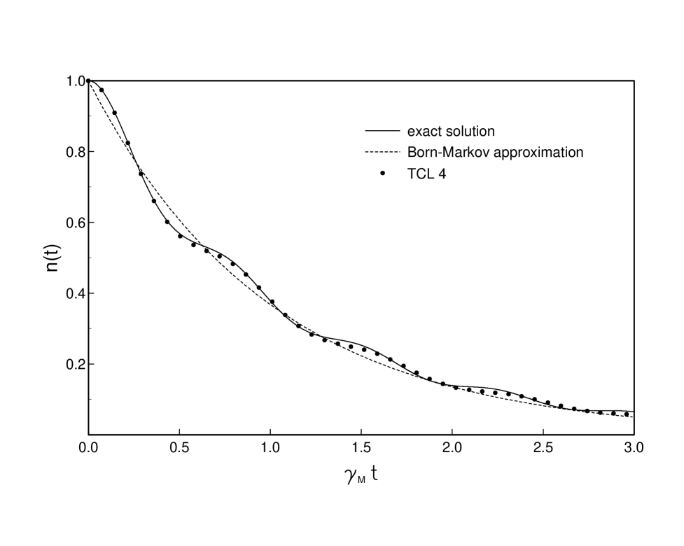
FIG. 1.: Normalized occupation number $n(t)=\langle a^{\dagger}a\rangle(t)/\langle a^{\dagger}a\rangle(0)$ of the BEC in the atomic trap. Plotted are Born-Markov approximation, exact solution and perturbation expansion to 4th order in the coupling strength $\Gamma=5\times 10^{4}s^{-1}$. This leads to a ratio of time scales $t_{\text{sys}}/t_{\text{res}}=16$.

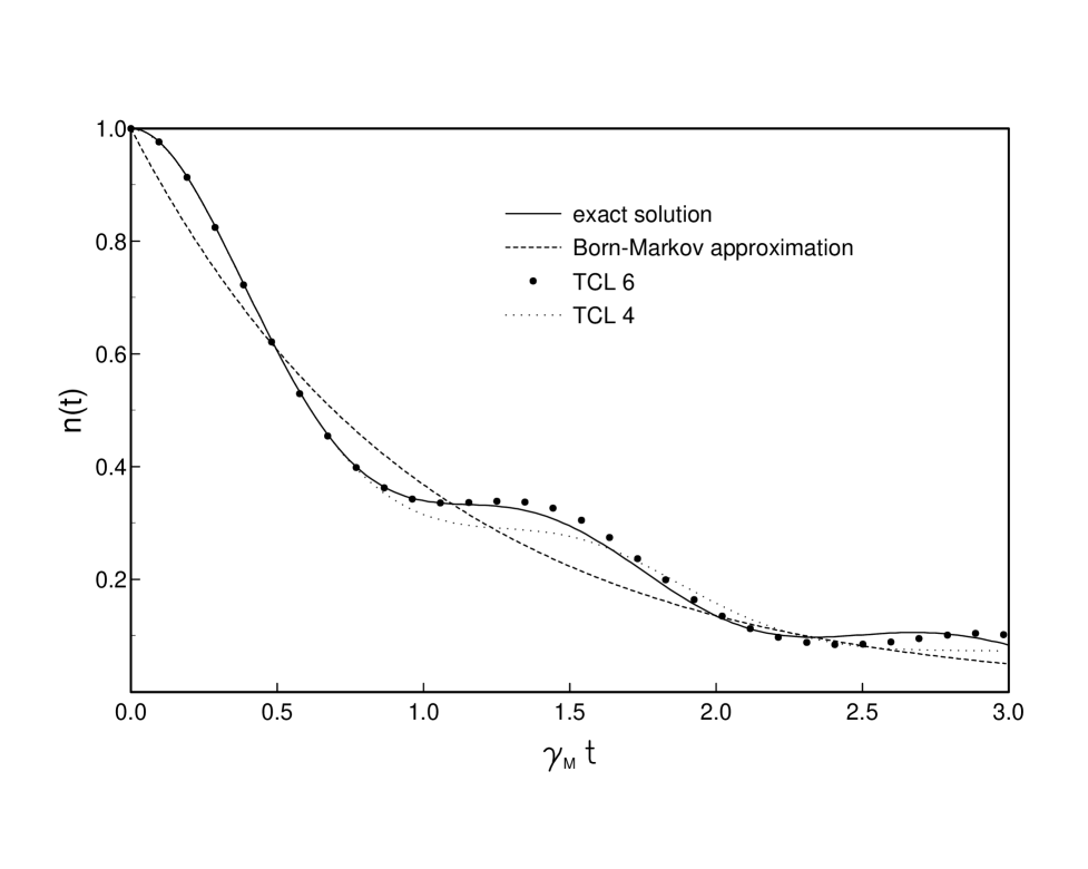
FIG. 2.: The normalized occupation number $n(t)=\langle a^{\dagger}a\rangle(t)/\langle a^{\dagger}a\rangle(0)$ of the BEC: exact results and the results from the Born-Markov approximation, resp., from 4th and 6th order perturbation theory. The parameter $\Gamma=10^{5}s^{-1}$ is chosen such that the ratio of time scales becomes $t_{\text{res}}/t_{\text{sys}}=8$.

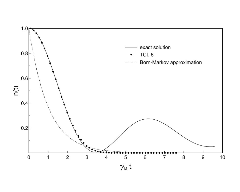
FIG. 3.: Normalized occupation number $n(t)=\langle a^{\dagger}a\rangle(t)/\langle a^{\dagger}a\rangle(0)$ of the BEC: Born-Markov approximation, exact solution and perturbation expansion to 6th order in the coupling strength $\Gamma=10^{6}s^{-1}$. This leads to a ratio of time scales $t_{\text{res}}/t_{\text{sys}}=0.8$.

FIG. 4.: Comparison of decay rates. Plotted are Born-Markov, exact decay rates and the decay rates in 4th and 6th order perturbation theory. The value of the coupling strength is $\Gamma=5\times 10^{4}s^{-1}$.

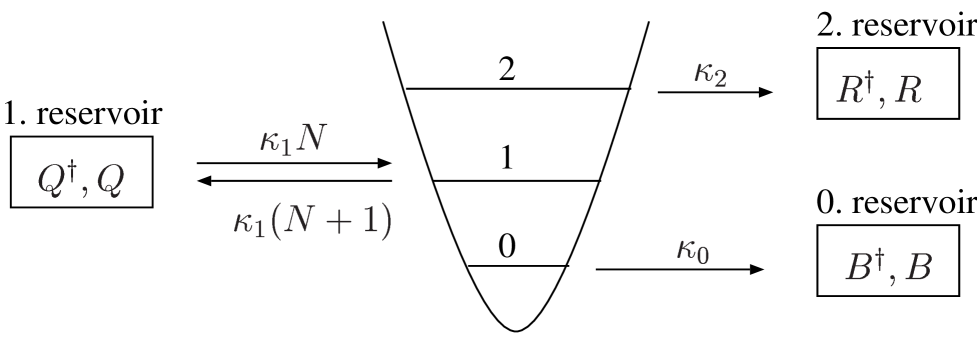
FIG. 5.: Our simplified model of a cw atom laser consists of a pump mode 1, the ground state mode 0 which is occupied from the Bose-Einstein condensate and the weakly bound mode 2 from which the atoms are strongly coupled out.

FIG. 6.: Occupation number $n(t)=\langle a^{\dagger}a\rangle(t)$ of the BEC in an atomic trap in the case of a continuous wave atom laser. Plotted are the Born-Markov approximation and the results of a non-Markovian perturbative expansion of the output coupling to second and fourth order in the coupling strength.

REFERENCES

- [1] E.mail: Heinz-Peter.Breuer@physik.uni-freiburg.de
- [2] E.mail: Daniel.Faller@physik.uni-freiburg.de
- [3] E.mail: Bernd.Kappler@physik.uni-freiburg.de
- [4] E.mail: Francesco.Petruccione@physik.uni-freiburg.de
- [5] K. B. Davis et al., Phys. Rev. Lett. 75, 3969 (1995).
- [6] M. H. Anderson et al., Science 269, 198 (1995).
- [7] M.-O. Mewes et al., Phys. Rev. Lett. 78, 582 (1997).
- [8] M. R. Andrews et al., Science 275, 637 (1997).
- [9] E. W. Hagley et al., Science 283, 1706 (1999).
- [10] I. Bloch, T. W. Hänsch, and T. Esslinger, Phys. Rev. Lett. 82, 3008 (1999).
- [11] D. S. Durfee and W. Ketterle, Optics Express 2, 299 (1998).
- [12] G. B. Lubkin, Physics Today 52, 17 (1999).
- [13] M. Holland et al., Phys. Rev. A 54, 1757 (1996).
- [14] O. Zobay and P. Meystre, Phys. Rev. A 57, 4710 (1998).
- [15] M. G. Moore and P. Meystre, Journal of Modern Optics 44, 1815 (1997).
- [16] A. M. Guzman, M. G. Moore, and P. Meystre, Phys. Rev. A 53, 977 (1996).
- [17] H. M. Wiseman and M. J. Collett, Phys. Lett. A 202, 246 (1995).
- [18] G. M. Moy, J. J. Hope, and C. M. Savage, Phys. Rev. A 59, 667 (1999).
- [19] S. Chaturvedi and F. Shibata, Zeitschrift für Physik B 35, 297 (1979).
- [20] F. Shibata and T. Arimitsu, Journal of the Physical Society of Japan 49, 891 (1980).
- [21] H. P. Breuer, B. Kappler, and F. Petruccione, Phys. Rev. A 59, 1633 (1999).
- [22] G. Lindblad, Commun. Math. Phys. 48, 119 (1976).
- [23] G. M. Moy, J. J. Hope, and C. M. Savage, Phys. Rev. A 55, 3631 (1997).
- [24] G. M. Moy and C. M. Savage, Phys. Rev. A 56, 1087 (1997).
- [25] J. J. Hope, Phys. Rev. A 55, 2531 (1997).
- [26] J. J. Hope, Ph.D. thesis, The Australian National University, 1998, unpublished.
- [27] M. W. Jack, M. Naraschewski, M. J. Collett, and D. F. Walls, Phys. Rev. A 59, 2962 (1999).
- [28] M. O. Mewes, Phys. Rev. Lett. 77, 416 (1996).
- [29] H. Carmichael, An Open Systems Approach to Quantum Optics, Lecture Notes in Physics m18 (Springer-Verlag, Berlin, Heidelberg, New York, 1993).
- [30] H. P. Breuer and F. Petruccione, Phys. Rev. Lett. 74, 3788 (1995), Phys. Rev. E 52, 428 (1995)
- [31] M. G. Moore and P. Meystre, Phys. Rev. A 56, 2989 (1997).