BA-TH/00-390

Decoherence vs entropy in neutron interferometry

P. Facchi,¹ A. Mariano² and S. Pascazio²

¹Atominstitut der Österreichischen Universitäten, Stadionallee 2, A-1020, Wien, Austria

²Dipartimento di Fisica, Università di Bari

and Istituto Nazionale di Fisica Nucleare, Sezione di Bari

I-70126 Bari, Italy

PACS: 03.65.Bz, 03.75.Be, 03.75.Dg

Abstract

We analyze the coherence properties of polarized neutrons, after they have interacted with a magnetic field or a phase shifter undergoing different kinds of statistical fluctuations. We endeavor to probe the degree of disorder of the distribution of the phase shifts by means of the loss of quantum mechanical coherence of the neutron. We find that the notion of entropy of the shifts and that of decoherence of the neutron do not necessarily agree. In some cases the neutron wave function is more coherent, even though it has interacted with a more disordered medium.

I Introduction

The notion of decoherence has attracted increasing attention in the literature of the last few years [1, 2]. The loss of quantum mechanical coherence undergone by a quantum system, as a consequence of its interaction with a given environment, can be discussed in relation to many different physical phenomena and has deepened our comprehension of fundamental issues, disclosing unexpected applications as well as innovative technology.

Neutron physics (neutron optics in particular) has played an important role in this context, both on theoretical and experimental grounds. Non-classical states are readily obtained, for instance by splitting and then superposing wavepackets in an interferometer [3] or different spin states in a magnetic field [4, 5], and are of great significance in the investigation of fundamental quantum mechanical properties. The aim of this paper is to investigate the coherence features of neutron wave packets, by making use of the Wigner function [6], in analogy with concepts and techniques that are routinely used in quantum optics [7]. The studies of the last few years have shown that non-classical states are fragile against statistical fluctuations [8, 9]: the analysis of situations where these states display robustness during the interaction with noisy environments is therefore of great practical interest.

The main motivation of this work is to use the coherence properties of the wave function as a “probe” to check the degree of disorder of an environment. A similar idea was first proposed, as far as we know, in the context of quantum chaos and Feynman integrals [10]. One might naively expect that a neutron ensemble suffers a greater loss of quantum coherence by interacting with an increasingly disordered environment: intuitively, a more disordered environment should provoke more randomization of the phase of the wave function, which in turn implies more quantum decoherence. As we shall see, this is not always true: some of the results to be discussed below are rather counterintuitive and at variance with naive expectation. In some cases the neutron wave function is more coherent, even though it has interacted with a more disordered medium. This statement can be given a precise quantitative meaning in terms of the entropy of the medium and of a “decoherence parameter” that will be defined for the neutron density matrix.

II Preliminaries

The Wigner quasidistribution function [6] can be defined in terms of the density matrix $\rho$ as

$$W(x,k)=\frac{1}{2\pi}\int d\xi\;e^{-ik\xi}\langle x+\xi/2|\rho|x-\xi/2\rangle,$$ (1)

where $x$ and $p=\hbar k$ are the position and momentum of the particle. One easily checks that the Wigner function is normalized to unity and its marginals represent the position and momentum distributions

$${\rm Tr}\rho=\int dx\;dk\;W(x,k)=1,$$ (2)

$$P(x)=\langle x|\rho|x\rangle=\int dk\;W(x,k),$$ (3)

$$P(k)=\langle k|\rho|k\rangle=\int dx\;W(x,k).$$ (4)

Notice that

$$\int dx\;dk\;W(x,k)^{2}=\frac{{\rm Tr}\rho^{2}}{2\pi}.$$ (5)

In this paper we shall consider a one-dimensional system (the extension to 3 dimensions is straightforward) and assume that the wave function is well approximated by a Gaussian

$$\psi(x) = \langle x|\psi\rangle=\frac{1}{(2\pi\delta^{2})^{1/4}}\exp\left[-\frac{(x-x_{0})^{2}}{4\delta^{2}}+ik_{0}x\right],$$ (6)

$$\phi(k) = \langle k|\psi\rangle=\frac{1}{(2\pi\delta_{k}^{2})^{1/4}}\exp\left[-\frac{(k-k_{0})^{2}}{4\delta_{k}^{2}}-i(k-k_{0})x_{0}\right]$$ (7)

$$= \left(\frac{2\delta^{2}}{\pi}\right)^{1/4}\exp\left[-\delta^{2}(k-k_{0})^{2}-i(k-k_{0})x_{0}\right],$$ (8)

where $\psi(x)$ and $\phi(k)$ are the wave functions in the position and momentum representation, respectively, $\delta$ is the spatial spread of the wave packet, $\delta_{k}\delta=1/2$, $x_{0}$ is the initial average position of the particle and $p_{0}=\hbar k_{0}$ its average momentum. The two functions above are both normalized to one: normalization will play an important role in our analysis and will never be neglected. The Wigner function for the state (6)-(8) is readily calculated

$$W(x,k)=\frac{1}{\pi}\exp\left[-\frac{(x-x_{0})^{2}}{2\delta^{2}}\right]\exp\left[-2\delta^{2}(k-k_{0})^{2}\right].$$ (9)

In this paper we will focus on two physical situations. In the first one, a polarized neutron acquires a phase shift $\Delta$, either by going through a phase shifter or by crossing a magnetic field parallel to its spin. In the second one, a polarized neutron is divided in two states, either in an interferometer or by crossing a magnetic field perpendicular to its spin. The latter situation is physically most interesting, for it yields non-classical states, whose coherence properties are of great interest.

A Single Gaussian

If a Gaussian wave packet undergoes a phase shift $\Delta$, the resulting Wigner function reads

$$W(x,k,\Delta)=\frac{1}{\pi}\exp\left[-\frac{(x-x_{0}+\Delta)^{2}}{2\delta^{2}}\right]\exp\left[-2\delta^{2}(k-k_{0})^{2}\right].$$ (10)

Physically, this is achieved either by placing a phase shifter in the neutron path, or by injecting a polarized neutron in a constant magnetic field parallel to its spin. In both cases, the total energy of the neutron is conserved. In the latter case, if the field has intensity $B$ and is contained in a region of length $L$, the neutron kinetic energy in the field changes by $\Delta E=-|\mu|B$, where $|\mu|$ is the neutron magnetic moment. This entails a change in average momentum $\Delta k=m\mu B/\hbar^{2}k_{0}$ and a phase shift proportional to $\Delta\equiv L\Delta k/k_{0}$. When it leaves the field, the neutron acquires again the initial kinetic energy.

B Double Gaussian

Consider now a neutron wave packet that is split and then recombined in an interferometer, with a phase shifter placed in one of the two routes. The Wigner function in the ordinary channel (transmitted component) is readily computed:

$$W^{\rm int}(x,k,\Delta) = \frac{1}{4\pi}\exp[-2\delta^{2}(k-k_{0})^{2}]\left[\exp\left(-\frac{\left(x-x_{0}+\Delta\right)^{2}}{2\delta^{2}}\right)\right.$$ (12)

$$\left.+\exp\left(-\frac{\left(x-x_{0}\right)^{2}}{2\delta^{2}}\right)+2\exp\left(-\frac{\left(x-x_{0}+\frac{\Delta}{2}\right)^{2}}{2\delta^{2}}\right)\cos(k\Delta)\right].$$

Notice that, for $\Delta\neq 0$, it is not normalized to unity (some neutrons end up in the extraordinary channel—reflected component) and that for $\Delta=0$ (no phase shifter) one recovers (9).

A similar result is obtained when a polarized (say, $+y$) neutron crosses a magnetic field aligned along an orthogonal direction (say, $+z$). The total neutron energy is conserved, but due to Zeeman splitting the two spin states in the direction of the $B$ field have different kinetic energies and travel with different speeds. This is a situation typically encountered in the so-called longitudinal Stern-Gerlach effect [4] and in neutron spin-echo experiments [5] (except that we are not considering the second half of the evolution, with an opposite $B$ field that recombines the two spin states). An experimental realization of this situation was investigated very recently [11]. If the initial wave function is

$$|\Psi\rangle=|\psi\rangle\otimes|+\rangle_{y}=|\psi\rangle\otimes\left(\frac{1}{\sqrt{2}}|+\rangle_{z}+\frac{i}{\sqrt{2}}|-\rangle_{z}\right),$$ (13)

where $|\pm\rangle_{\alpha}\;(\alpha=x,y,z)$ represents spin up/down in direction $\alpha$, the final state in the position representation, after crossing the $B$-field, reads

$$\langle x|\Psi\rangle=\frac{1}{\sqrt{2}}\;\psi\left(x+\frac{\Delta}{2}\right)\otimes|+\rangle_{z}+\frac{i}{\sqrt{2}}\;\psi\left(x-\frac{\Delta}{2}\right)\otimes|-\rangle_{z}.$$ (14)

If only the $+y$-spin component is observed (“post selection” of the initial spin component [12]) the probability amplitude is

$$_{y}\langle+,x|\Psi\rangle=\frac{1}{2}\left[\psi\left(x+\frac{\Delta}{2}\right)+\psi\left(x-\frac{\Delta}{2}\right)\right],$$ (15)

and the Wigner function is readily computed as

$$W^{\rm magn}(x,k,\Delta) = \frac{1}{4\pi}\exp[-2\delta^{2}(k-k_{0})^{2}]\left[\exp\left(-\frac{\left(x-x_{0}-\frac{\Delta}{2}\right)^{2}}{2\delta^{2}}\right)\right.$$ (17)

$$\left.+\exp\left(-\frac{\left(x-x_{0}+\frac{\Delta}{2}\right)^{2}}{2\delta^{2}}\right)+2\exp\left(-\frac{(x-x_{0})^{2}}{2\delta^{2}}\right)\cos(k\Delta)\right].$$

This result is slightly different from (12), because in this case both spin components undergo a phase shift ($\pm\Delta/2$). Once again, for $\Delta=0$ (no magnetic field) one reobtains (9).

We stress that in both cases the neutron wave packet has a natural spread $\delta_{t}=\sqrt{\delta^{2}+(\hbar t/2m\delta)^{2}}$ (due to its free evolution for a time $t\simeq mL/\hbar k_{0}$); however, this additional effect will be neglected, because, as proved in Appendix A, it is not relevant for the loss of quantum coherence.

III Fluctuating phase shift

The previous analysis refers to a rather idealized case, in which every neutron in the beam acquires a constant phase shift. This is clearly not a realistic situation, for it does not take into account the statistical fluctuations of the $B$ field or of the shifter in the transverse section of the beam. If, for any reason, the phase shift $\Delta$ fluctuates, the neutron beam will partially loose its quantum coherence and the Wigner function will be affected accordingly. We shall consider the case of “slow” fluctuations, in the sense that each neutron crosses an approximately static $B$ field (or a phase shifter of uniform length $L$), but the intensity of the field (or the length of the shifter) varies for different neutrons in the beam (different “events”). We will suppose that every neutron undergoes a shift $\Delta$ that is statistically distributed according to a distribution law $w(\Delta)$. The collective “degree of disorder” of the shifts $\Delta$ can be given a quantitative meaning in terms of the entropy

$$S=-\int d\Delta\;w(\Delta)\;\log(w(\Delta)).$$ (18)

On the other hand, the average Wigner function reads

$$W_{\rm m}(x,k)=\int d\Delta\;w(\Delta)\;W(x,k,\Delta)$$ (19)

and represents a partially mixed state. The coherence properties of the neutron ensemble can be analyzed in terms of a decoherence parameter [13]

$$\varepsilon=1-\frac{\mbox{Tr}\rho^{2}}{(\mbox{Tr}\rho)^{2}}=1-\frac{2\pi\int dx\;dk\;W_{\rm m}(x,k)^{2}}{\left(\int dx\;dk\;W_{\rm m}(x,k)\right)^{2}}.$$ (20)

This quantity measures the degree of “purity” of a quantum state: it is maximum when the state is maximally mixed (Tr$\rho^{2}<$Tr$\rho$) and vanishes when the state is pure (Tr$\rho^{2}=$Tr$\rho$): in the former case the fluctuations of $\Delta$ are large and the quantum mechanical coherence is completely lost, while in the latter case $\Delta$ does not fluctuate and the quantum mechanical coherence is perfectly preserved. The parameter (20) was introduced within the framework of the so-called “many Hilbert space” theory of quantum measurements [8, 2] and yields a quantitative estimate of decoherence. The related quantity Tr$\rho-$Tr$\rho^{2}$ (that might be called “idempotency defect”) was first considered by Watanabe [14] many years ago. A measure of information for a quantum system has been recently introduced, which is related to $\varepsilon$ and is more suitable than the Shannon entropy [15].

One might naively think that the two quantities $S$ and $\varepsilon$ should at least qualitatively agree: in other words, the loss of quantum mechanical coherence should be larger when the neutron beam interacts with fluctuating shifts of larger entropy. Such a naive expectation turns out to be incorrect. Our purpose is to investigate this problem. To this end, it is useful to consider some particular cases.

A Gaussian noise

We first assume that the shifts $\Delta$ fluctuate around their average $\Delta_{0}$ according to a Gaussian law:

$$w(\Delta)=\frac{1}{\sqrt{2\pi\sigma^{2}}}\exp\left[-\frac{(\Delta-\Delta_{0})^{2}}{2\sigma^{2}}\right],$$ (21)

where $\sigma$ is the standard deviation. The ratio $\sigma/\Delta_{0}$ is simply equal to the ratio $\delta B/B_{0}$ (or $\delta L/L_{0}$), $\delta B$ ($\delta L$) being the standard deviation of the fluctuating magnetic field (length of phase shifter) and $B_{0}$ ($L_{0}$) its average. The entropy of (21) is readily computed from (18)

$$S=\frac{1}{2}\log(2\pi e\sigma^{2})$$ (22)

and is obviously an increasing function of $\sigma$.

1 Single Gaussian

Consider now a neutron described by a Gaussian wave packet. If the phase shift $\Delta$ fluctuates according to (21), the average Wigner function is readily computed by (19), (10) and (21),

$$W_{\rm m}(x,k)=\frac{1}{\pi}\;\sqrt{\frac{\delta^{2}}{\delta^{2}+\sigma^{2}}}\;\exp[-2\delta^{2}(k-k_{0})^{2}]\;\exp\left[-\frac{(x-x_{0}+\Delta_{0})^{2}}{2(\delta^{2}+\sigma^{2})}\right]$$ (23)

and its marginals (3)-(4) are easily evaluated

$$P(x) = \frac{1}{\sqrt{2\pi(\delta^{2}+\sigma^{2})}}\exp\left[-\frac{(x-x_{0}+\Delta_{0})^{2}}{2(\delta^{2}+\sigma^{2})}\right],$$ (24)

$$P(k) = \sqrt{\frac{2\delta^{2}}{\pi}}\exp\left[-2\delta^{2}(k-k_{0})^{2}\right].$$ (25)

Notice that the momentum distribution (25) is unaltered and identical to $|\phi(k)|^{2}$ in (8): obviously, the energy of each neutron does not change. Observe on the other hand the additional spread in position $\delta^{\prime}=\sqrt{\delta^{2}+\sigma^{2}}$ (Figure 1) and notice that the Wigner function and its marginals are always normalized to one.

The decoherence parameter (20) can be analytically evaluated

$$\varepsilon=1-\sqrt{\frac{\delta^{2}}{\delta^{2}+\sigma^{2}}}$$ (26)

and is a monotonic function of $\sigma$ for every value of $\delta$. This behavior is in qualitative agreement with that of the entropy (22). As expected, a more entropic distribution of phase shifts entails a greater loss of quantum mechanical coherence for the neutron ensemble. The behavior of $\epsilon$ vs $\delta$ and $\sigma$ is shown in Figure 2(a).

2 Double Gaussian in an interferometer

Consider now the double Gaussian state (12), obtained when a neutron beam crosses an interferometer. The average Wigner function (19) reads

$$W_{\rm m}^{\rm int}(x,k)=\frac{\exp[-2\delta^{2}(k-k_{0})^{2}]}{4\pi}\left\{\sqrt{\frac{\delta^{2}}{\delta^{2}+\sigma^{2}}}\exp\left[-\frac{(x+\Delta_{0})^{2}}{2(\delta^{2}+\sigma^{2})}\right]+\exp\left[-\frac{x^{2}}{2\delta^{2}}\right]\right.$$ (27)

$$\left.+2\sqrt{\frac{\delta^{2}}{\delta^{2}+\frac{\sigma^{2}}{4}}}\exp\left[-\frac{\left(x+\frac{\Delta_{0}}{2}\right)^{2}+k^{2}\delta^{2}\sigma^{2}}{2\left(\delta^{2}+\frac{\sigma^{2}}{4}\right)}\right]\cos\left(k\frac{2\delta^{2}\Delta_{0}-x\sigma^{2}}{2\left(\delta^{2}+\frac{\sigma^{2}}{4}\right)}\right)\right\},$$ (28)

where we set $x_{0}=0$ for simplicity. Its marginals (3)-(4) can both be computed analytically; in particular, the momentum probability distribution reads

$$P(k)=\sqrt{\frac{\delta^{2}}{2\pi}}\exp\left[-2\delta^{2}(k-k_{0})^{2}\right]\left[1+\exp\left(-\frac{k^{2}\sigma^{2}}{2}\right)\cos(k\Delta_{0})\right].$$ (29)

As one can see from Figure 3(a), interference is exponentially suppressed at high values of $k$ and the oscillating part of the Wigner function is bent towards the negative $x$-axis. This is due to the $x$-dependence of the cosine term in (28) that entails different frequencies for different values of $x$. The decoherence parameter (20) reads

$$\varepsilon = 1-\frac{1}{4N^{2}}\left[\frac{1}{4}\left(1+\sqrt{\frac{\delta^{2}}{\delta^{2}+\sigma^{2}}}\right)+\sqrt{\frac{\delta^{2}}{4\delta^{2}+2\sigma^{2}}}\left(\exp\left[-\frac{\Delta_{0}^{2}}{4\delta^{2}+2\sigma^{2}}\right]+\exp\left[-\frac{2k_{0}^{2}\delta^{2}\sigma^{2}}{2\delta^{2}+\sigma^{2}}\right]\right)\right]$$ (30)

$$- \frac{1}{2N^{2}}\left[\sqrt{\frac{\delta^{2}}{4\delta^{2}+\sigma^{2}}}\exp\left[-\frac{\Delta_{0}^{2}+4k_{0}^{2}\delta^{2}\sigma^{2}}{2(4\delta^{2}+\sigma^{2})}\right]\cos\left[\frac{4k_{0}\Delta_{0}\delta^{2}}{4\delta^{2}+\sigma^{2}}\right]\right.$$ (32)

$$\left.+\frac{\delta^{2}}{4\delta^{2}+\sigma^{2}}\exp\left[-\frac{\Delta_{0}^{2}+4k_{0}^{2}\delta^{2}\sigma^{2}}{4\delta^{2}+\sigma^{2}}\right]\cos\left[\frac{8k_{0}\Delta_{0}\delta^{2}}{4\delta^{2}+\sigma^{2}}\right]\right]$$

$$- \frac{\delta^{2}}{N^{2}\sqrt{16\delta^{4}+12\delta^{2}\sigma^{2}+\sigma^{4}}}\exp\left[\frac{(2\delta^{2}+\sigma^{2})(\Delta_{0}^{2}+4k_{0}^{2}\delta^{2}\sigma^{2})}{16\delta^{4}+12\delta^{2}\sigma^{2}+\sigma^{4}}\right]\cos\left[\frac{4k_{0}\Delta_{0}\delta^{2}(4\delta^{2}+3\sigma^{2})}{16\delta^{4}+12\delta^{2}\sigma^{2}+\sigma^{4}}\right],$$ (33)

where the normalization

$$N = \int dx\;dk\;W_{\rm m}(x,k)$$ (34)

$$= \frac{1}{2}\left[1+\sqrt{\frac{\delta^{2}}{\delta^{2}+\frac{\sigma^{2}}{4}}}\exp\left(-\frac{\Delta_{0}^{2}+4\delta^{2}\sigma^{2}k_{0}^{2}}{8\left(\delta^{2}+\frac{\sigma^{2}}{4}\right)}\right)\cos\left(\frac{\delta^{2}}{\delta^{2}+\frac{\sigma^{2}}{4}}k_{0}\Delta_{0}\right)\right]$$ (35)

represents the probability of detecting a neutron in the ordinary channel. The explicit expression (33) of the decoherence parameter is involved and difficult to understand. Therefore, $\varepsilon$ is shown in Figure 2(b) as a function of $\delta$ and $\sigma$ for fixed values of $k_{0}$ and $\Delta_{0}$: somewhat surprisingly, for some values of $\delta$, even though the noise $\sigma$ increases, the decoherence $\varepsilon$ decreases.

Observe also that $\varepsilon$ never reaches unity: $\varepsilon\leq 3/4$. This is due to the fact that one of the two Gaussians does not undergo any fluctuations (there is a fluctuating phase shifter in only one of the two routes of the interferometer): therefore a part of the Wigner function is not affected by noise, as one can see in Figure 3(a). We shall comment again on the peculiar features of $\varepsilon$ in a while.

3 Double Gaussian in a magnetic field

If we consider a polarized neutron beam interacting with a $B$ field perpendicular to its spin, Eq. (17) yields

$$W_{\rm m}^{\rm magn}(x,k,\Delta)=\frac{\exp[-2\delta^{2}(k-k_{0})^{2}]}{4\pi}\left\{\sqrt{\frac{\delta^{2}}{\delta^{2}+\frac{\sigma^{2}}{4}}}\exp\left[-\frac{(x-\frac{\Delta_{0}}{2})^{2}}{2(\delta^{2}+\frac{\sigma^{2}}{4})}\right]\right.$$ (36)

$$\left.\;+\;\sqrt{\frac{\delta^{2}}{\delta^{2}+\frac{\sigma^{2}}{4}}}\exp\left[-\frac{(x+\frac{\Delta_{0}}{2})^{2}}{2(\delta^{2}+\frac{\sigma^{2}}{4})}\right]+2\exp\left[-\frac{x^{2}}{2\delta^{2}}-\frac{k^{2}\sigma^{2}}{2}\right]\cos(k\Delta_{0})\right\},$$ (37)

This Wigner function has the same $k$-marginal (29) as the previous one (although the $x$-marginals are different). Also in this case, one observes a strong suppression of interference at large values of momentum [9, 11, 13], but without $x$-dependence in the cosine. See Figure 3(b). In this case, the decoherence parameter (20) reads

$$\varepsilon = 1-\frac{1}{4N^{2}}\;\sqrt{\frac{\delta^{2}}{4\delta^{2}+\sigma^{2}}}\;\exp\left(-\frac{\Delta_{0}^{2}+4k_{0}^{2}\delta^{2}\sigma^{2}}{4\delta^{2}+\sigma^{2}}\right)\;\cos\left(\frac{8k_{0}\Delta_{0}\delta^{2}}{4\delta^{2}+\sigma^{2}}\right)$$ (40)

$$-\frac{1}{4N^{2}}\;\sqrt{\frac{\delta^{2}}{4\delta^{2}+\sigma^{2}}}\;\left[1+\exp\left(-\frac{\Delta_{0}^{2}}{4\delta^{2}+\sigma^{2}}\right)+\exp\left(-\frac{4k_{0}^{2}\delta^{2}\sigma^{2}}{4\delta^{2}+\sigma^{2}}\right)\right]$$

$$-\frac{4}{N^{2}}\;\frac{\delta^{2}}{8\delta^{2}+\sigma^{2}}\;\exp\left(-\frac{\Delta_{0}^{2}+4k_{0}^{2}\delta^{2}\sigma^{2}}{8\delta^{2}+\sigma^{2}}\right)\;\cos\left(\frac{8k_{0}\Delta_{0}\delta^{2}}{8\delta^{2}+\sigma^{2}}\right).$$

Again, the explicit expression of the decoherence parameter is complicated and depends on several physical parameters; it is therefore convenient to concentrate on a particular case. An experimental realization of a fluctuating shift (according to a given statistical law) is easier with the magnetic field arrangement discussed in Section II B. Let us therefore consider the experiment [11], in which a polarized ($+y$) neutron enters a magnetic field, perpendicular to its spin, of intensity $B_{0}=0.28$mT, confined in a region of length $L=57$cm. The average neutron wavenumber is $k_{0}=1.7\cdot 10^{10}$m^-1 and its coherence length (defined by a chopper) is $\delta=1.1\cdot 10^{-10}$m. By travelling in the magnetic field, the two neutron spin states are separated by a distance $\Delta_{0}=2m\mu B_{0}L/\hbar^{2}k_{0}^{2}=16.1\cdot 10^{-10}$m, one order of magnitude larger than $\delta$. The behavior of $\varepsilon$ in (40) is shown in Figure 2(c) for these experimental values: observe that for $\delta\gtrsim 3$Å  $\epsilon$ is not a monotonic function of $\sigma$: in other words, for some values of the parameters, even though the noise $\sigma$ increases, the decoherence $\epsilon$ decreases. This is at variance with the behavior of the entropy (22) and with what one might naively expect. We conclude that, in general, both for a double Gaussian in an interferometer and in a magnetic field, the behavior of $\varepsilon$ does not agree with that of the entropy.

B Sinusoidal fluctuations with increasingly less rational frequencies

In order to shed some more light on the results of the previous subsection, let us consider a different example, that is more convenient for an experimental perspective. Suppose that the phase shift changes according to the law

$$\Delta(t)=\Delta_{0}+\Delta_{1}[\sin(\Omega t)+\sin(r_{j}\Omega t)].$$ (41)

where $t$ is time, $\Omega$ a frequency much smaller than $v_{0}/L$, the inverse time of flight of the neutron in the shifter’s region, $\Delta_{0}$ the mean phase shift, $\Delta_{1}(\ll\Delta_{0})$ the “fluctuation” width (see below) and $r_{j}\;(0<r_{j}<1)$ a real number. For the neutron ensemble (the beam) the shifts will be distributed according to law

$$w(\Delta)=\int dt\;f(t)\;\delta(\Delta-\Delta(t)),$$ (42)

where $f(t)$ is the probability density function of the stochastic variable $t$. In our case, $f(t)=1/T$ in $(0,T)$, where $T(\gg\Omega^{-1})$ is a sufficiently large time interval. In such a case, by making use of (42), the Wigner function can be expressed as an ergodic average

$$W_{\rm m}(x,k)=\int d\Delta\;w(\Delta)\;W(x,k,\Delta)=\frac{1}{T}\int_{T}dt\;W(x,k,\Delta(t)).\quad(T\;\mbox{large})$$ (43)

We stress that $\Delta$ is treated like a random variable although, strictly speaking, the underlying process is deterministic. However, this is not a conceptual difficulty: in practice, one just treats the neutron ensemble in an experimental run without looking at the correlations among different neutrons. The same effects on the neutron ensemble would be obtained by first generating a random variable $t$, uniformly distributed in $(0,T)$, then constructing the additional random variable $\Delta$ according to (41) and finally accumulating all neutrons in the experimental run. In this way different neutrons are uncorrelated. The distribution law of the shifts (41) can be obtained by means of a $B$-field

$$B(t)=B_{0}+B_{1}\left[\sin(\Omega t)+\sin(r_{j}\Omega t)\right].$$ (44)

Like in the previous section, we assume that $B$ is a slowly varying function of time, so that each neutron experiences a static field during its interaction. Observe that the scheme proposed in (41)-(43) is not difficult to realize experimentally. On the other hand, it would be complicated to obtain the same distribution of shifts with a phase shifter placed in one of the two routes of an interferometer.

We will study the coherence properties of the neutron beam when it crosses a magnetic field made up of two “increasingly less rational” frequencies, by choosing

$$r_{j}=\frac{f_{j}}{f_{j+1}},$$ (45)

where $f_{j}$ are the Fibonacci numbers

$$f_{j+1}=f_{j}+f_{j-1}\qquad(f_{0}=f_{1}=1).$$ (46)

This particular choice is motivated by the (naive) expectation that an oscillating magnetic field (44) composed of mutually less rational frequencies should provoke more decoherence on the neutron ensemble. Once again, this expectation will turn out to be incorrect. The ratios (45) tend to the golden mean (the “most irrational” number [16]) as $j$ increases

$$r_{j}\stackrel{{\scriptstyle j\to\infty}}{{\longrightarrow}}r_{\infty}=\frac{\sqrt{5}-1}{2}.$$ (47)

In general, one cannot obtain an analytic expression for the probability density function (42); however, an accurate numerical evaluation of $w(\Delta)$ is possible: for every finite value of $j$, $r_{j}$ is a rational number, so that one can integrate (42) over the interval $T=f_{j+1}2\pi/\Omega$. In Figure 4 we show the results of our numerical analysis. The distribution function $w(\Delta)$ has a finite number of (integrable) divergences in its interval of definition; as the order in the Fibonacci sequence becomes higher, the number of divergences in the interval grows. In the $j\to\infty$ limit, i.e. for the golden mean $r_{\infty}=(\sqrt{5}-1)/2$, it is possible to apply the theorem on averages for the ergodic motion on a torus [17] and find an analytical expression of $w(\Delta)$ in terms of an elliptic integral of first kind (see Appendix B). The resulting distribution is a smooth function with only one (integrable) divergence in $\Delta=0$ and is plotted in Fig. 4(f).

By applying the same technique utilized for the numerical evaluation of $w$, the entropy is computed according to the formula

$$S=-\int d\Delta\;w(\Delta)\;\log(w(\Delta))=-\frac{1}{T}\int_{T}dt\;\log[w(\Delta(t))],$$ (48)

which is easily obtained by Eqs. (18) and (42) (using the value $T=f_{j+1}2\pi/\Omega$ for the numerical evaluation).

The decoherence parameter is computed from Eq. (20), first with the Wigner function (10) (single Gaussian) and then with the Wigner function (17) (double Gaussian in a magnetic field): in both formulas, we used Eq. (43) and set $\Delta_{0}=16.1\cdot 10^{-10}$m, $\Delta_{1}=2\cdot 10^{-10}$m and the same numerical values of the previous subsection for $k_{0}$ and $\delta$ [11]. Our results are summarized in Table 1 and Figure 5.

We notice that, although, for $j=1,...,5$, $S$ is a monotonically increasing function of the Fibonacci number in the sequence, $\varepsilon$ reaches a maximum for $r_{j}=3/5$ (i.e., $j=3$). It is remarkable that the maximum is obtained for the same Fibonacci ratio in both cases (single and double Gaussian). Once again, the behavior of entropy and decoherence are qualitatively different. Figure 5 should be compared to Figure 2: it is worth noting that in the case analyzed in this section, unlike in Section III A, the behavior of entropy and decoherence do not agree even when the neutron state is a single Gaussian (namely, a “classical” state).

IV Conclusions

Decoherence is a very useful concept, that has recently been widely investigated and has turned out to be very prolific. It is intuitively related to the loss of “purity” of a quantum mechanical state and can be given a quantitative definition, as in (20). However, we have seen that the very notion of decoherence is delicate: in particular, it is not correct to think that a quantum system, by interacting with an increasingly “disordered” environment, will suffer an increasing loss of quantum coherence. Our analysis has been performed by assuming that each neutron, during an experimental run, interacts with a constant magnetic field: the neutron beam, on the average, undegoes decoherence. This “quasistatic” approximation is only a working hypothesis and will be relaxed in future work. As emphasized at the beginning of Sec. III B, it is easy to achieve experimentally in the limit $\Omega\ll v_{0}/L$, where $\Omega$ is a characteristic frequency of the fluctuation and $(v_{0}/L)^{-1}$ the time of flight of the neutron in the phase shifter or in the magnetic field. This approximation also simplifies (both conceptually and technically) our theoretical analysis, without however having a substantial influence on our general conclusions. It is worth stressing, in this respect, that the decoherence parameter, defined in (20), depends on the interaction and not on the free Hamiltonian, at least in the physical situations investigated here (see Appendix A).

Our quantitative definition of decoherence depends, as it should, on the very characteristics of the experimental setup: the decoherence parameter is defined in terms of the average Wigner function (or equivalently the density matrix) of the neutron ensemble, after the interaction with the apparatus. An experimental check of the features of the Wigner functions discussed in this paper would require its tomographic observation. Similar techniques are commonly applied in quantum optics [18] and would be available in neutron optics as well, in particular for the experimental arrangement discussed in Section III B. However, we think that a better comprehension of the effects analyzed in this paper could probably be achieved by studying the marginals (or possibly some other tomographic projection) of the Wigner function and the visibility of the interference pattern. Additional work is in progress in this direction. From an experimental perspective, an analysis of decoherence effects along the guidelines discussed here would be challenging: although the concepts of decoherence and entropy are intuitively related, they display some interesting differences. If properly understood, those situations in which a larger noise yields a more coherent quantum ensemble might lead to unexpected applications.

Appendix A

We prove that the decoherence parameter (20), under rather general conditions, does not depend on the free evolution of a quantum system. Let the Hamiltonian of a quantum system be

$$H=H_{0}+H_{1}(\alpha),$$ (A.1)

where $H_{0}$ and $H_{1}$ are the free and interaction Hamiltonians, respectively, and $\alpha$ is a c-number (that can fluctuate according to a given statistical law). We assume that

$$[H_{0},H_{1}(\alpha)]=iC,\qquad\mbox{with}\qquad[H_{0},C]=[H_{1}(\alpha),C]=0,$$ (A.2)

where $C$ is in general an operator (independent of $\alpha$), so that ($\hbar=1$)

$$e^{-it(H_{0}+H_{1}(\alpha))}=e^{it^{2}C/2}e^{-itH_{0}}e^{-itH_{1}(\alpha)}.$$ (A.3)

Consider now the density matrix at time $t$,

$$\rho_{\alpha}(t)=e^{-it(H_{0}+H_{1}(\alpha))}\;\rho_{0}\;e^{it(H_{0}+H_{1}(\alpha))},$$ (A.4)

where $\rho_{0}$ is the initial density matrix. From Eq. (A.3)

$$\rho_{\alpha}(t)=e^{it^{2}C/2}\;e^{-itH_{0}}\;e^{-itH_{1}(\alpha)}\;\rho_{0}\;e^{itH_{1}(\alpha)}\;e^{itH_{0}}e^{-it^{2}C/2}$$ (A.5)

and the average over $\alpha$ yields

$$\overline{\rho(t)}=e^{it^{2}C/2}\;e^{-itH_{0}}\left(\int d\alpha\;w(\alpha)\;{\rm e}^{-itH_{1}(\alpha)}\;\rho_{0}\;{\rm e}^{itH_{1}(\alpha)}\right)e^{itH_{0}}e^{-it^{2}C/2},$$ (A.6)

where $w(\alpha)$ is the distribution function and the bar denotes average. Therefore

$${\rm Tr}\left[\overline{\rho(t)}\right]={\rm Tr}\left[\overline{\rho_{\rm int}(t)}\right],$$ (A.7)

where $\rho_{\rm int}$ is the density matrix in the following interaction picture:

$$\rho_{\rm int}(t)=e^{itH_{0}-it^{2}C/2}\;\rho(t)\;e^{-itH_{0}+it^{2}C/2}=e^{-itH_{1}(\alpha)}\;\rho_{0}\;e^{itH_{1}(\alpha)}.$$ (A.8)

This proves that the trace of the average density matrix does not depend on the free evolution. The result (A.7) can be generalized to any function of the average density matrix

$${\rm Tr}\left[f\left(\overline{\rho(t)}\right)\right]={\rm Tr}\left[f\left(\overline{\rho_{\rm int}(t)}\right)\right].$$ (A.9)

This shows that the decoherence parameter defined in (20) does not depend on the free evolution:

$$\varepsilon=\varepsilon_{\rm int},$$ (A.10)

as claimed at the end of Sec. II. This result can be applied to the case studied in Sec. III, where $H_{0}=\frac{p^{2}}{2m},H_{1}=-\mbox{\boldmath$\mu$}\cdot\mbox{\boldmath$B$}$ and the parameter $\alpha$ is the intensity of the magnetic field $B$ (whose direction is supposed constant). Notice that we are considering wave packets that interact with a constant and homogeneous field $B$ from the initial time $t=0$ to the final time $t\simeq mL/\hbar k_{0}$, so that condition (A.2) is fulfilled. The case of a neutron wave packet in an interferometer is analogous, if we assume that the phase shifter simply yields a phase (optical potential approximation).

Appendix B

We compute here the distribution function (42) when $f(t)=1/T$ and $\Delta(t)$ changes according to (41), in the $j=\infty$ limit (47). The function $w(\Delta)$ has a finite number of (integrable) divergences in its interval of definition. Notice that, as the order in the Fibonacci sequence becomes higher, the number of divergences in the interval grows and the numerical evaluation of the distribution function becomes more difficult. Let us introduce the two-component vector

$$\mbox{\boldmath$\varphi$}_{j}(t)=(\varphi_{1},\;\varphi_{2})=\mbox{\boldmath$\omega$}_{j}t,\quad\mbox{where}\quad\mbox{\boldmath$\omega$}_{j}=(\Omega,\;r_{j}\Omega).$$ (B.1)

The vector $\mbox{\boldmath$\varphi$}_{j}$ performs a (quasi)periodic motion on the two-dimensional torus $T^{2}$. In particular, for every finite value of $j$ the frequencies are dependent, i.e. $\omega_{2}/\omega_{1}=r_{j}\in\mathbb{Z}$, and the orbits are closed. For larger values of $j$ the number of windings in a period increases and the length of the periodic orbit becomes larger. In the $j\to\infty$ limit, the two frequencies become independent and the resulting motion on the 2-torus becomes ergodic: the trajectory is everywhere dense and uniformly distributed on $T^{2}$. In this case, according to the theorem on averages [17], the time average of every integrable function $f(\mbox{\boldmath$\varphi$})$ (where $\mbox{\boldmath$\varphi$}\equiv\mbox{\boldmath$\varphi$}_{\infty}$) coincides with its space average, i.e.

$$\lim_{T\to\infty}\frac{1}{T}\int_{0}^{T}dt\;f(\mbox{\boldmath$\varphi$}(t))=\frac{1}{(2\pi)^{2}}\int_{0}^{2\pi}d\varphi_{1}\int_{0}^{2\pi}d\varphi_{2}\;f(\mbox{\boldmath$\varphi$}).$$ (B.2)

Applying Eq. (B.2) to the function

$$f(\mbox{\boldmath$\varphi$})=\delta(\Delta-\Delta_{1}[\sin\varphi_{1}+\sin\varphi_{2}])$$ (B.3)

we obtain

$$w(\Delta) = \lim_{T\to\infty}\frac{1}{T}\int_{0}^{T}\;dt\;\delta(\Delta-\Delta_{1}[\sin(\Omega t)+\sin(r_{\infty}\Omega t]))$$ (B.4)

$$= \frac{1}{(2\pi)^{2}}\int_{0}^{2\pi}d\varphi_{1}\int_{0}^{2\pi}d\varphi_{2}\;\delta(\Delta-\Delta_{1}[\sin\varphi_{1}+\sin\varphi_{2}])$$ (B.5)

$$= \frac{1}{\Delta_{1}}\int_{-1}^{+1}ds\;P_{S}(s)\;P_{S}(\Delta/\Delta_{1}-s),$$ (B.6)

where $P_{S}$ is the sine distribution

$$P_{S}(s)=\frac{1}{2\pi}\int_{0}^{2\pi}d\varphi\;\delta(s-\sin\varphi)=\frac{1}{\pi\sqrt{1-s^{2}}}.$$ (B.7)

After some algebraic manipulation one finds

$$w(\Delta)=\frac{2}{\pi^{2}\Delta_{1}}\;F\left(\arcsin\frac{1}{\sqrt{1+\frac{|\Delta|}{2\Delta_{1}}}},\sqrt{1-\left(\frac{\Delta}{2\Delta_{1}}\right)^{2}}\right),$$ (B.8)

where $F(\beta,\gamma)$ is the elliptic integral of first kind [19]

$$F(\beta,\gamma)=\int_{0}^{\beta}\;d\alpha\;\frac{1}{\sqrt{1-\gamma^{2}\sin^{2}\alpha}}.$$ (B.9)

The limiting distribution function (B.8) is plotted in Fig. 4(f).

Observe that in Fig. 4(a-f) the number of divergences increases so quickly that, in the $j=\infty$ limit (golden mean), $w(\Delta)$ becomes a smooth function with only one (integrable) divergence in $\Delta=0$ (indeed $w(\Delta)\sim\log(8\Delta_{1}/|\Delta|)/\pi^{2}\Delta_{1}$ for $\Delta\to 0$). In this sense Berry et al. coined the epigram “stocasticity is the ubiquity of catastrophe” [20]. (Incidentally, notice the similarity of Fig. 4 with Fig. 12 of [20].)

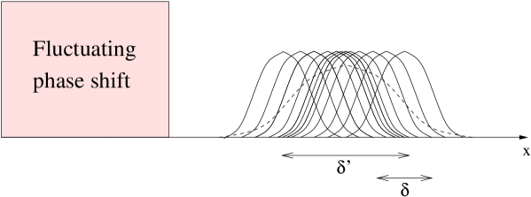
FIG. 1.: If the phase shift fluctuates, each wave packet acquires a different shift. This is pictorially represented in the figure, where different outgoing wave packets are displayed, each associated with a single neutron (“event”). The average Wigner function is given by Eq. (23).

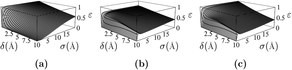
FIG. 2.: Decoherence parameter vs coherence length of the wave packet $\delta$(Å) and standard deviation of the fluctuation $\sigma$(Å). (a) Gaussian wave packet. (b) Double Gaussian in an interferometer, with $\Delta_{0}=16.1$Å. (c) Double Gaussian in a magnetic field, with $\Delta_{0}=16.1$Å. In all cases $k_{0}=1.7$Å^-1. Observe that in case (a) the decoherence parameter is a monotonic function of $\sigma$ for every value of $\delta$, while this is not true for cases (b) and (c). Notice also that in case (b) the decoherence parameter never reaches unity ($\varepsilon\leq 3/4$): this is due to the fact that only one Gaussian (in one branch of the interferometer) undergoes statistical fluctuations [see Figure 3(a)].

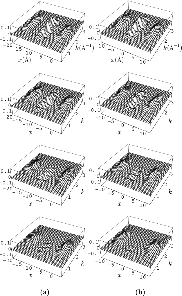
FIG. 3.: Wigner functions for different values of the standard deviation $\sigma$ in (21). (a) Double Gaussian in an interferometer (28). (b) Double Gaussian in a magnetic field (37). From top to bottom, $\sigma=0,0.6,1.2,1.8$Å. The values of the other parameters are $x_{0}=0$, $k_{0}=1.7$Å^-1, $\delta=1.1$Å, $\Delta_{0}=16.1$Å. Position $x$ and momentum $k$ are measured in Å and Å^-1, respectively. Notice the strong suppression of interference at large values of momentum, both in (a) and (b). In case (a) only one of the two Gaussians interacts with the fluctuating phase shifter; moreover, the interference term in (28) depends on $x$ and the oscillating part of the Wigner function is bent towards the negative $x$-axis.

FIG. 4.: Phase shift $\Delta$ in (41) and distribution function $w(\Delta)$ in (42), for different values of $r_{j}$: (a) $r_{1}=1/2$; (b) $r_{2}=2/3;$ (c) $r_{3}=3/5;$ (d) $r_{4}=5/8;$ (e) $r_{5}=8/13;$ (f) $r_{\infty}=(\sqrt{5}-1)/2$. In each figure $\Delta_{1}=2$ (we set $\Delta_{0}=0$ for clarity of presentation): above, phase shift $\Delta(t)$; below, distribution function $w(\Delta)$. Notice that, by increasing $j$ (index of the Fibonacci sequence), the two frequencies become mutually “less rational,” the phase shift $\Delta(t)$ becomes more irregular and its distribution function $w(\Delta)$ more uniform. [The entropy behaves accordingly, increasing for $j=1,\ldots,5$ (see Fig. 5(a))]. Notice that the number of divergences of the distribution function increases with $j$; as shown in Appendix B, in the $j=\infty$ limit, the distribution becomes continuous with only one (logarithmic) divergence in $\Delta=0$ and can be expressed as an elliptic integral (B.8).

FIG. 5.: (a) Entropy (48) vs $j$ (index in the Fibonacci sequence). (b) Decoherence parameter (20) vs $j$: case of a single Gaussian. (c) Decoherence parameter (20) vs $j$: case of a double Gaussian in a magnetic field. Notice that, while the entropy is an increasing function of $j$ for $j=1,\ldots,5$, the decoherence parameter displays a maximum at $j=3$, both for a single and a double Gaussian.

TABLE I.: Entropy and Decoherence

$j$	$r_{j}$	$S$	$\varepsilon$ (single Gaussian)	$\varepsilon$ (double Gaussian)
1	1/2	1.6165	0.52894	0.59545
2	2/3	1.7398	0.53166	0.62478
3	3/5	1.7458	0.53199	0.63184
4	5/8	1.9051	0.53173	0.62695
5	8/13	1.9434	0.53173	0.62695

REFERENCES

- [1] D. Giulini et al, Decoherence and the Appearance of a Classical World in Quantum Theory (Springer, Berlin, 1996).
- [2] M. Namiki, S. Pascazio and H. Nakazato, Decoherence and Quantum Measurements (World Scientific, Singapore, 1997).
- [3] H. Bonse and H. Rauch, eds., Neutron Interferometry (Clarendon, Oxford, 1979); G. Badurek, H. Rauch and A. Zeilinger, Matter Wave Interferometry (North-Holland, Amsterdam, 1988); H. Rauch and S. A. Werner, Neutron Interferometry: Lessons in Experimental Quantum Mechanics (Oxford University Press, Oxford, 2000).
- [4] F. Mezei, Physica B151, 74 (1988); R. Golub, R. Gähler and T. Keller, Am. J. Phys. 62, 779 (1994).
- [5] F. Mezei, Z. Phys. 25, 146 (1972); Neutron Spin Echo, Lecture Notes in Physics 128 (Springer Verlag, Berlin, 1980).
- [6] E. Wigner, Phys. Rev. 40, 749 (1932); M. Hillery et al, Phys. Rep. 106, 121 (1984).
- [7] R. J. Glauber, Phys. Rep. 130, 2766 (1963).
- [8] M. Namiki and S. Pascazio, Phys. Lett. A147, 430 (1990); Phys. Rev. A44, 39 (1991).
- [9] H. Rauch and M. Suda, Physica B241-243, 157 (1998); J. Appl. Phys. B60, 181 (1995); H. Rauch, M. Suda and S. Pascazio, Physica B267, 277 (1999).
- [10] N. Saito in Quantum Physics, Chaos Theory and Cosmology, M. Namiki ed. (AIP, New York, 1996) p. 275; M. Namiki (private communication); H. Nakazato et al, Phys. Lett. A222, 130 (1996); N. Saito and H. Makino, Quantum chaos, ergodicity, and quantum measurement. General considerations, preprint Waseda University, Japan (2000).
- [11] G. Badurek et al, Optics Comm. 179, 13 (2000).
- [12] H. Rauch et al, Phys. Rev. A53, 902 (1996).
- [13] P. Facchi, A. Mariano and S. Pascazio, Acta Phys. Slov. 49, 677 (1999); Physica B276-278, 970 (2000).
- [14] S. Watanabe, Z. Phys. 113, 482 (1939).
- [15] Č. Brukner and A. Zeilinger, Phys. Rev. Lett. 83, 3354 (1999).
- [16] A. M. Ozorio de Almeida, Hamiltonian Systems: Chaos and Quantization (Cambridge University Press, Cambridge, 1988), Section 5.3.
- [17] V. I. Arnol’d, Mathematical methods of classical mechanics (Springer Verlag, Berlin, 1989), §51.
- [18] W. Vogel and D. G. Welsh, Lectures on Quantum Optics (Akademie Verlag/VCH Publishers, Berlin, 1994); W. P. Schleich, M. Pernigo and F. Le Kien, Phys. Rev. A44 2172 (1991); G. Breitenbach, S. Schiller and J. Mlynek, Nature 387, 471 (1997); D. Vitali, P. Tombesi and G. J. Milburn, Phys. Rev. A57, 4930 (1998).
- [19] I. S. Gradshteyn and I. M. Ryzhik, Table of Integrals, Series, and Products (Academic Press, San Diego, 1994), §8.111.
- [20] M. V. Berry, N. L. Balazs, M. Tabor and A. Voros, Ann. Phys. 122, 26 (1979).