Geometric Quantum Mechanics

Abstract

The manifold of pure quantum states can be regarded as a complex projective space endowed with the unitary-invariant Riemannian geometry of Fubini and Study. According to the principles of geometric quantum mechanics, the detailed physical characteristics of a given quantum system can be represented by specific geometrical features that are selected and preferentially identified in this complex manifold. In particular, any specific feature of projective geometry gives rise to a physically realisable characteristic in quantum mechanics. Here we construct a number of examples of such geometrical features as they arise in the state spaces for spin-$\frac{1}{2}$, spin-1, and spin-$\frac{3}{2}$ systems, and for pairs of spin-$\frac{1}{2}$ systems. A study is undertaken on the geometry of entangled states, and a natural measure is assigned to the degree of entanglement of a given state for a general multi-particle system. The properties of this measure are analysed in detail for the entangled states of a pair of spin-$\frac{1}{2}$ particles, thus enabling us to determine the structure of the space of maximally entangled states. With the specification of a quantum Hamiltonian, the resulting Schrödinger trajectories induce an isometry of the Fubini-Study manifold. For a generic quantum evolution, the corresponding Killing trajectory is quasiergodic on a toroidal subspace of the energy surface. When the dynamical trajectory is lifted orthogonally to Hilbert space, it induces a geometric phase shift on the wave function. The uncertainty of an observable in a given state is the length of the gradient vector of the level surface of the expectation of the observable in that state, a fact that allows us to calculate higher order corrections to the Heisenberg relations. A general mixed state is determined by a probability density function on the state space, for which the associated first moment is the density matrix. The advantage of the idea of a general state is in its applicability in various attempts to go beyond the standard quantum theory, some of which admit a natural phase-space characterisation.

Keywords: Quantum phase space; projective geometry;
quantum entanglement; Kibble-Weinberg theory

1 Introduction

The line of investigation which we refer to as ‘Geometric Quantum Mechanics’ originated over two decades ago in the work of Kibble (1978, 1979), who showed how quantum theory could be formulated in the language of Hamiltonian phase-space dynamics. This was a remarkable development inasmuch as previously it was believed by physicists that classical mechanics has a natural Hamiltonian phase-space structure, to which one had to apply a suitable quantisation procedure to produce a very different kind of structure, namely, the complex Hilbert space of quantum mechanics together with a family of linear operators, corresponding to physical observables. However, with the advent of geometric quantum mechanics it has become difficult to sustain this point of view, and quantum theory has come to be recognised much more as a self-contained entity.

A notable attempt to codify the quantisation procedure in a rigourous mathematical framework was pursued in the geometric quantisation program (see, e.g., Woodhouse 1992). Geometric quantum mechanics, however, is not concerned with the quantisation procedure, as such, but accepts quantum theory as given. Indeed, from a modern perspective the current flows in reverse, and a major objective is to understand how the classical world emerges from quantum theory. Thus, in contrast to the aforementioned ‘geometric quantisation’ program, what we really need might be more appropriately called a ‘geometric classicalisation’ program.

To this extent, there may even be grounds for arguing that the notion of quantisation is superfluous. Present thinking on these issues is based on a special relationship between classical and quantum mechanics distinct from the quantisation idea, namely, that quantum theory possesses an intrinsic mathematical structure equivalent to that of Hamiltonian phase-space dynamics, only the underlying phase-space is not that of classical mechanics, but rather the quantum mechanical state space itself, i.e., what we call the ‘space of pure states’.

The approach to quantum mechanics via its natural phase-space geometry initiated by Kibble offers insights into many of the more enigmatic aspects of the theory: linear superposition of states, Schrödinger evolution, quantum entanglement, quantum probability laws, uncertainty relations, geometric phases, and the collapse of the wave function. One of the goals of this article is to illustrate in geometrical terms the interplay between these aspects of quantum theory.

The plan of the paper is as follows. In §2-4 we introduce the projective geometric framework, and review the main features of the quantum phase space. In §5 the phase space of a spin-1 system is studied, and in §6 we look at a spin-$\frac{3}{2}$ system, relating the properties of this system to the geometry of the twisted cubic curve in $CP^{3}$. In §7 we develop a geometric theory of entangled states and discuss the properties of quantum measurements made on such systems. This theory is extended in §8-10 where we introduce a new measure of entanglement, and explore its applications.

In §11-14 we consider quantum dynamics from a geometric view, and demonstrate in particular a quasiergodic property satisfied by the Schrödinger trajectories. We show that the theory of geometric phase has a natural characterisation in this setting, thus allowing us to introduce a quantum mechanical analogue of the Poincare integral invariant. Then in §15 we examine the status of mixed states in the geometric framework of relevance to quantum statistical mechanics, and discuss the merits of general states characterised by density functions on the quantum phase space.

Following the original observations of Kibble, many authors (see, e.g., Heslot 1985; Anandan $\&$ Aharonov 1990; Cirelli, et. al. 1990; Gibbons 1992, 1997; Gibbons $\&$ Phole 1993; Hughston 1995, 1996; Ashtekar $\&$ Schilling 1998; Brody $\&$ Hughston 1999a; Field $\&$ Hughston 1999; Adler $\&$ Horwitz 1999) have contributed to the further development of geometric quantum mechanics, and in doing so have demonstrated that this methodology not only provides new insights into the workings of the quantum world as we presently understand it, but also acts as a base from which extensions of standard quantum theory can be developed, some of which we shall touch upon briefly towards the end of this article, in §16.

2 Projective state space

Let us begin by reviewing briefly how quantum mechanics is ordinarily formulated. A physical system is represented by a wave function $\psi({\bf x},t)$, which for each time $t$ belongs to a complex Hilbert space ${\cal H}$. We also require a set of linear operators on ${\cal H}$, corresponding to observables. The wave function characterises the ‘state’ of the system at time $t$. In the case of a single particle of mass $m$ moving in Euclidean 3-space under the influence of a potential $\phi({\bf x})$, the evolution of the system is given by Schrödinger’s wave equation

$${\rm i}\hbar\frac{\partial}{\partial t}\psi({\bf x},t)\ =\ \left(-\frac{1}{2m}\nabla^{2}+\phi({\bf x})\right)\psi({\bf x},t)\ .$$

Given an initial condition $\psi({\bf x},0)$, the Schrödinger equation determines the development of the state, in terms of which we can then calculate the expectation of any observable.

Physical properties of the system depend on the wave function only up to an overall complex factor. For instance, suppose we consider an observation to determine whether the particle lies in a region $D$ in ${\bf R}^{3}$. We define the linear operator $\chi_{{}_{D}}$, the characteristic function for $D$, by the property $\chi_{{}_{D}}\psi({\bf x})=\psi({\bf x})$ for ${\bf x}\in D$ and $\chi_{{}_{D}}\psi({\bf x})=0$ for ${\bf x}\notin D$. Thus $\chi_{{}_{D}}$ ‘truncates’ the wave function outside $D$. In particular, $\chi_{{}_{D}}$ has two eigenvalues, 1 and 0, corresponding to eigenfunctions concentrated on $D$ and on the complement of $D$ in ${\bf R}^{3}$. The probability of an affirmative result for a measurement to determine whether the particle lies in $D$ is given by the expectation of the operator $\chi_{{}_{D}}$, that is,

$${\rm E}[\chi_{{}_{D}}]\ =\ \frac{\int_{{\bf R}^{3}}{\bar{\psi}}({\bf x})\chi_{{}_{D}}\psi({\bf x})d^{3}x}{\int_{{\bf R}^{3}}{\bar{\psi}}({\bf x})\psi({\bf x})d^{3}x}\ .$$

In this case, we note that the probability density function

$$p({\bf x})\ =\ \frac{{\bar{\psi}}({\bf x})\psi({\bf x})}{\int_{{\bf R}^{3}}{\bar{\psi}}({\bf x})\psi({\bf x})d^{3}{\bf x}}$$

on ${\bf R}^{3}$ is independent of the phase and scale of $\psi({\bf x})$. In other words, the state of the system is not given by $\psi({\bf x})$ itself, but rather by an equivalence class modulo transformations of the form

$$\psi({\bf x},t)\ \rightarrow\ e^{{\rm i}\lambda(t)}\psi({\bf x},t)$$

for any complex time-dependent function $\lambda(t)$. For this reason, we say the state is given, at any time, by a ‘ray’ through the origin in ${\cal H}$. The space of such rays is called projective Hilbert space, denoted ${\cal PH}$. All of the operations of quantum mechanics can be referred to ${\cal PH}$ directly, without consideration of ${\cal H}$ itself. For example, the Schrödinger equation is not invariant under a change of phase and scale for $\psi({\bf x})$, whereas the projective Schrödinger equation

$${\rm i}\hbar\left[\psi({\bf y})\frac{\partial\psi({\bf x})}{\partial t}-\psi({\bf x})\frac{\partial\psi({\bf y})}{\partial t}\right]\ = \ -\frac{1}{2m}\left[\psi({\bf y})\nabla^{2}\psi({\bf x})-\psi({\bf x})\nabla^{2}\psi({\bf y})\right]$$

$$\ +\left[\phi({\bf x})-\phi({\bf y})\right]\psi({\bf x})\psi({\bf y})$$

is, in fact, invariant under such transformations. Had Schrödinger elected to present this relation as his wave equation, none of the physical consequences would have differed.

3 Pure states

There is a beautiful geometry associated with the projective Hilbert space ${\cal PH}$ which is so compelling in its richness that, in our opinion, all physicists should become acquainted with it. The basic idea can be sketched as follows. For simplicity we use an index notation for the Hilbert space ${\cal H}$. Instead of $\psi({\bf x})$ we write $\psi^{\alpha}$, where the Greek index $\alpha$ labels components of the Hilbert-space vector with respect to a basis. This notation serves us equally well whether ${\cal H}$ is finite or infinite dimensional. The highly effective use of the index notation for Hilbert space was first popularised by Geroch (1970). For the complex conjugate of $\psi^{\alpha}$ we write ${\bar{\psi}}_{\alpha}$. The ‘downstairs’ index reminds us that ${\bar{\psi}}_{\alpha}$ is a ‘bra’ vector, i.e., it belongs to the dual of the vector space to which $\psi^{\alpha}$ belongs.

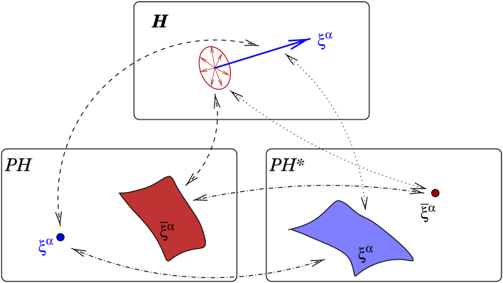
Figure 1: Hermitian correspondence. A pure quantum mechanical state corresponds to a ray through the origin $O$ in complex Hilbert space ${\cal H}$. Such a ray is given by a Hilbert space vector $\xi^{\alpha}$, specified up to proportionality, which can also be used as a set of ‘homogeneous coordinates’ for a point in the projective Hilbert space ${\cal PH}$. The states $\psi^{\alpha}$ orthogonal to $\xi^{\alpha}$ constitute a projective hyperplane in ${\cal PH}$, with the equation ${\bar{\xi}}_{\alpha}\psi^{\alpha}=0$. This hyperplane corresponds to a point ${\bar{\xi}}_{\alpha}$ in the dual projective space ${\cal PH}^{*}$.

The usual inner product between $\psi^{\alpha}$ and ${\bar{\psi}}_{\alpha}$ can be written ${\bar{\psi}}_{\alpha}\psi^{\alpha}$, with an implied summation over the repeated index. In the case of a wave function, this is equivalent to $\int_{{\bf R}^{3}}{\bar{\psi}}({\bf x})\psi({\bf x})d^{3}x$, which in the Dirac bra-ket notation is $\langle{\bar{\psi}}|\psi\rangle$. By use of the index notation the Schrödinger equation can be represented in the compact form ${\rm i}\hbar\partial_{t}\psi^{\alpha}=H^{\alpha}_{\beta}\psi^{\beta}$, where $H^{\alpha}_{\beta}$ is the Hamiltonian operator, $\partial_{t}=\partial/\partial t$, and for the projective Schrödinger equation we have

$${\rm i}\hbar\psi^{[\alpha}\partial_{t}\psi^{\beta]}\ =\ \psi^{[\alpha}H^{\beta]}_{\gamma}\psi^{\gamma},$$

where the skew brackets indicate antisymmetrisation.

A Hilbert space vector $\xi^{\alpha}$ can also represent homogeneous coordinates for the corresponding point in the projective Hilbert space ${\cal PH}$. This is valid when we consider relations homogeneous in $\xi^{\alpha}$, for which the scale is irrelevant. For example the complex conjugate ${\bar{\xi}}_{\alpha}$ of a ‘point’ in ${\cal PH}$ can be represented by the linear subspace (hyperplane) of points $\psi^{\alpha}$ in ${\cal PH}$ satisfying ${\bar{\xi}}_{\alpha}\psi^{\alpha}=0$. The set of all such hyperplanes constitutes the dual space ${\cal PH}^{*}$. The points of ${\cal PH}^{*}$ correspond to hyperplanes in ${\cal PH}$. Conversely, the points of ${\cal PH}$ correspond to hyperplanes in ${\cal PH}^{*}$, as illustrated in Figure 1.

One of the advantages of the use of projective geometry in the present context is that it allows us to represent states (points) and dual states (hyperplanes) as geometrical objects coexisting in the same space ${\cal PH}$. The complex conjugation operation, in particular, determines a Hermitian correspondence between points and their orthogonal hyperplanes.

4 Superposition of states

The join of two distinct points $\xi^{\alpha}$ and $\eta^{\alpha}$ in ${\cal PH}$ is a complex projective line, represented by points in ${\cal PH}$ of the form

$$\psi^{\alpha}\ =\ A\xi^{\alpha}+B\eta^{\alpha}\ ,$$

where $A$ and $B$ are complex numbers, not both zero. A neat way of characterising this line is the tensor $L^{\alpha\beta}=\xi^{[\alpha}\eta^{\beta]}$. Physically, $L^{\alpha\beta}$ represents the system of all possible quantum mechanical superpositions of the states $\xi^{\alpha}$ and $\eta^{\alpha}$. To see that $L^{\alpha\beta}$ represents a line, consider a finite dimensional case where ${\cal PH}=CP^{n}$. Then, because of the skew-symmetry of $L^{\alpha\beta}$ it has $\frac{1}{2}n(n+1)$ complex components, which can be viewed as the line coordinates of the given line. The fundamental property of these line coordinates is that their ratios are independent of the choice of the two points $\xi^{\alpha}$ and $\eta^{\alpha}$, in such a way that all points on the given line are treated on an equal footing.

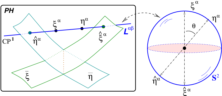
Figure 2: Transition probability. The join of two states $\xi^{\alpha}$ and $\eta^{\alpha}$ in projective Hilbert space ${\cal PH}$ is a complex projective line $CP^{1}$: $L^{\alpha\beta}=\xi^{[\alpha}\eta^{\beta]}$. The points on $L^{\alpha\beta}$ represent superpositions of $\xi^{\alpha}$ and $\eta^{\alpha}$. Such a line is intrinsically a real 2-manifold with spherical topology. The conjugate hyperplanes ${\bar{\xi}}_{\alpha}$ and ${\bar{\eta}}_{\alpha}$ intersect $L^{\alpha\beta}$ at points ${\hat{\xi}}^{\alpha}$ and ${\hat{\eta}}^{\alpha}$ in ${\cal PH}$. The angle $\theta$ determined by the cross ratio $\cos^{2}(\theta/2)=\xi^{\alpha}{\bar{\eta}}_{\alpha}\eta^{\beta}{\bar{\xi}}_{\beta}/\xi^{\gamma}{\bar{\xi}}_{\gamma}\eta^{\delta}{\bar{\eta}}_{\delta}$ induces a metrical geometry on $S^{2}$, for which $\theta$ is the usual angular distance, and ${\hat{\xi}}^{\alpha}$ is antipodal to $\xi^{\alpha}$.

The simplest situation in which a probabilistic idea arises in quantum theory is also the simplest situation in which the concept of the ‘distance’ between two states arises. The transition probability for the states $\xi^{\alpha}$ and $\eta^{\alpha}$ determines an angle $\theta$ as follows:

$$\cos^{2}\frac{1}{2}\theta\ =\ \frac{\xi^{\alpha}{\bar{\eta}}_{\alpha}\eta^{\beta}{\bar{\xi}}_{\beta}}{\xi^{\gamma}{\bar{\xi}}_{\gamma}\eta^{\delta}{\bar{\eta}}_{\delta}}\ .$$

Clearly, $\theta$ is independent of the scale and phase of $\xi^{\alpha}$ and $\eta^{\alpha}$. This angle defines a distance between the states $\xi^{\alpha}$ and $\eta^{\alpha}$ in ${\cal PH}$. If the states coincide, then $\theta=0$; for orthogonal states we have $\theta=\pi$, the maximum distance.

Suppose we set $\theta=ds$ and $\xi^{\alpha}=\psi^{\alpha}$, $\eta^{\alpha}=\psi^{\alpha}+d\psi^{\alpha}$. By use of the expression for the transition probability, expanded to second order, we find that the infinitesimal distance $ds$ between two neighbouring states is

$$ds^{2}\ =\ 8\frac{\psi^{[\alpha}d\psi^{\beta]}{\bar{\psi}}_{[\alpha}d{\bar{\psi}}_{\beta]}}{({\bar{\psi}}_{\gamma}\psi^{\gamma})^{2}}\ ,$$

an expression known to geometers as the Fubini-Study metric (Kobayashi $\&$ Nomizu 1969; Arnold 1989). This expression is well-defined both in finite and infinite dimensions. The introduction of the Fubini-Study geometry illustrates how the notions of probability and distance become interlinked, once quantum theory is formulated in a geometric manner. The geodesic distance with respect to the Fubini-Study metric determines the transition probability between two states. Indeed, the nontrivial metrical geometry of the Fubini-Study manifold is responsible for the ‘peculiarities’ of the quantum world, and in what follows we shall see various examples of this phenomenon.

5 Spin measurements

The specification of a physical system implies further geometrical structure on the state space. Indeed, the point of view we suggest is that all the relevant physical details of a quantum system can be represented by additional projective geometrical features. Here and in subsequent sections we shall illustrate this point with several examples. Let us first consider the spin degrees of freedom of a nonrelativistic spin-1 particle, as represented by a symmetric spinor $\phi^{AB}$ ($A,B=0,1$). The relevant Hilbert space has three dimensions, and we denote the corresponding projective Hilbert space $CP^{2}$. A symmetric spinor has a natural decomposition $\phi^{AB}=\alpha^{(A}\beta^{B)}$, where $\alpha^{A}$ and $\beta^{A}$ are called ‘principal spinors’, and round brackets denote symmetrisation. There is a special conic ${\cal C}$, corresponding to degenerate spinors of the form $\phi^{AB}=\psi^{A}\psi^{B}$ for some repeated principal spinor $\psi^{A}$.

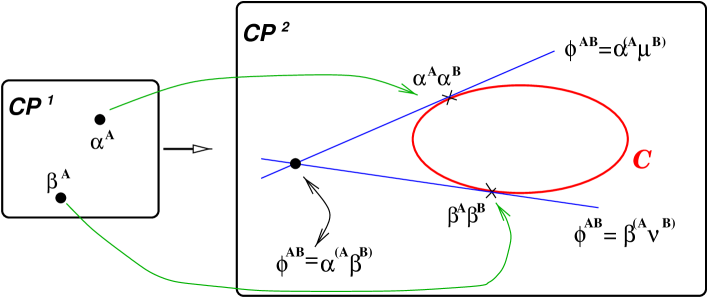
Figure 3: Spin-1 particle. A symmetric spinor $\phi^{AB}$ has three independent components which act as homogeneous coordinates for $CP^{2}$. The image of the map ${\cal C}:\ CP^{1}\rightarrow CP^{2}$, defined by $\{\psi^{A}\in CP^{1}\}\rightarrow\{\psi^{A}\psi^{B}\in CP^{2}\}$ determines a curve ${\cal C}$ in $CP^{2}$. The tangent to ${\cal C}$ at the point $\phi^{AB}=\alpha^{A}\alpha^{B}$ in $CP^{2}$ consists of spinors of the form $\phi^{AB}=\alpha^{(A}\mu^{B)}$ for some $\mu^{A}$. The intersection of the lines tangent to the points $\alpha^{A}\alpha^{B}$ and $\beta^{A}\beta^{B}$ is the point $\alpha^{(A}\beta^{B)}$. Conversely, once a conic ${\cal C}$ is specified, a map ${\cal C}^{-1}$ is established from $CP^{2}$ to point-pairs in $CP^{1}$, called principal spinors. The points on ${\cal C}$ map to degenerate point-pairs. An analogous result holds for spin 2, which has striking applications in gravitational theory, first systematically explored by Penrose (1960).

The identification of ${\cal C}$ is sufficient to induce the structure of a spin-1 system on the state space, since through any generic point in $CP^{2}$ there are two lines tangent to ${\cal C}$, and the corresponding tangent points determine the principal spinors, up to scale, as shown in Figure 3. Alternatively, we can think of a conic ${\cal C}$ in $CP^{2}$ being represented by a map (see, e.g., Semple $\&$ Kneebone 1952) from $CP^{1}$ to $CP^{2}$ such that if $(t,u)$ are homogeneous coordinates on $CP^{1}$, we have

$${\cal C}:\ (t,u)\rightarrow(t^{2},tu,u^{2})\ ,$$

where $(t^{2},tu,u^{2})$ now represents homogeneous coordinates on $CP^{2}$. Because a complex projective line, in real dimensions, represents a sphere $S^{2}$ (cf. Figure 2), the specification of the spin direction determines a point on $S^{2}$, and hence on ${\cal C}$.

The conic is required to be compatible with the complex conjugation operation on the state space in the sense that if we conjugate a point of ${\cal C}$, then the resulting line is tangent to ${\cal C}$. The complex conjugate ${\bar{\phi}}_{AB}={\bar{\alpha}}_{(A}{\bar{\beta}}_{B)}$ of a general state corresponds to a complex projective line consisting of states of the form $P{\bar{\alpha}}^{A}{\bar{\alpha}}^{B}+Q{\bar{\beta}}^{A}{\bar{\beta}}^{B}$, where we define ${\bar{\alpha}}^{A}=\epsilon^{AB}{\bar{\alpha}}_{B}$ and ${\bar{\beta}}^{A}=\epsilon^{AB}{\bar{\beta}}_{B}$, with $\epsilon^{AB}$ the natural symplectic structure. The rules for the complex conjugation map c on spinors are as follows:

$$\left\{\begin{array}[]{l}{\bf c}(\alpha^{A})\ =\ {\bar{\alpha}}_{A}\\ {\bf c}({\bar{\alpha}}^{A})\ =\ -\alpha_{A}.\end{array}\right.$$

The latter identity arises since ${\bf c}({\bar{\alpha}}^{A})={\bf c}(\epsilon^{AB}{\bar{\alpha}}_{B})=\epsilon_{AB}\alpha^{B}=-\alpha_{A}$. Recall that for any spinor $\phi^{A}$ we have the relation $\phi^{A}=\epsilon^{AB}\phi_{B}$ and $\phi^{A}\epsilon_{AB}=\phi_{B}$, and that $\epsilon_{AB}$ satisfies $\epsilon_{AB}=-\epsilon_{BA}$ and $\epsilon_{AB}={\bar{\epsilon}}_{BA}$. If we take the complex conjugate of a state on ${\cal C}$, the resulting line is tangent to the conic at a point, which we call the conjugate of the original point on ${\cal C}$. This establishes a Hermitian correspondence between pairs of points on ${\cal C}$. For a state $\phi^{AB}=\psi^{A}\psi^{B}$ the conjugate line consists of states of the form $\lambda^{(A}{\bar{\psi}}^{B)}$ for arbitrary $\lambda^{A}$. This line touches the conic ${\cal C}$ at the point ${\bar{\psi}}^{A}{\bar{\psi}}^{B}$.

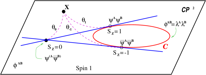
Figure 4: Spin measurement. The state space of a spin 1 system has a conjugation relation that associates to each point $\psi^{A}\psi^{B}$ on the special conic a conjugate point ${\bar{\psi}}^{A}{\bar{\psi}}^{B}$. The antipodal points $\psi^{A}$ and ${\bar{\psi}}^{A}$ on the corresponding 2-sphere select a direction in Euclidean 3-space. The three points $\psi^{A}\psi^{B}$, ${\bar{\psi}}^{A}{\bar{\psi}}^{B}$, and $\psi^{(A}{\bar{\psi}}^{B)}$ are eigenstates of the spin operator $S_{z}$ associated with this axis. The corresponding geodesic distances $\theta_{1}$, $\theta_{-1}$, $\theta_{0}$ to a generic state ${\bf X}\in CP^{2}$ determine the probabilities of the measurement outcomes for $S_{z}$ for a particle in the state ${\bf X}$.

Each choice of a point on ${\cal C}$, as noted above, determines a spin axis. For any spin axis there are three possible spin states, with eigenvalues $1,-1$ and $0$. The spin eigenstates are the points $\psi^{A}\psi^{B}$ and ${\bar{\psi}}^{A}{\bar{\psi}}^{B}$ on ${\cal C}$, having the eigenvalues 1 and $-1$, together with a third point $\psi^{(A}{\bar{\psi}}^{B)}$ obtained by intersecting the lines tangent to the conic ${\cal C}$ at the other two points, corresponding to eigenvalue 0, as indicated in Figure 4.

When a spin measurement is made, the initial state corresponds to a generic point ${\bf X}$ in $CP^{2}$, and the measurement is defined by a spin axis. The state then ‘jumps’ from its initial point to one of the three spin eigenstates associated with the choice of axis. Quantum theory, as such, states nothing about the “mechanism” whereby this jump is achieved. We can, however, compute the probabilities, and describe the result in geometrical terms. First we calculate the distance from ${\bf X}$ to each of the three spin eigenstates, by use of the Fubini-Study metric. This gives us three angles $\theta_{1}$, $\theta_{-1}$, and $\theta_{0}$. For each angle we compute $P(\theta)=\frac{1}{2}(1+\cos\theta)$, which gives us the probability of transition to that particular state. It is not obvious that the three probabilities computed in this way sum up to one, given any initial state in which the measurement is performed, but they do: this is a ‘miracle’ of the Fubini-Study geometry.

6 Spin-$\frac{3}{2}$ and the twisted cubic

We have seen that in the case of a projective plane, there is a conic ${\cal C}$, corresponding to degenerate spinors obtained by a special map from a projective line to a plane. On the other hand, in three-dimensional projective space $CP^{3}$ there are two different kinds of locus to be considered, each of which is in some respects a proper analogue of the conic, namely, the quadric surface $Q$ and the twisted cubic curve ${\cal T}$. While a surface is the locus of a variable point of space which has two complex degree of freedom, a curve is the locus of a variable point of space of one complex degree of freedom. When viewed as the state space of a quantum mechanical system, the quadric surface in $CP^{3}$ characterises the disentangled states of a pair of spin-$\frac{1}{2}$ particles, the geometry of which we shall study in some detail in subsequent sections.

The twisted cubic, the simplest nonplanar curve in projective geometry, on the other hand, plays an essential role in the geometry of the state space of a spin-$\frac{3}{2}$ particle. Analogous to the conic curve, the twisted cubic can be represented by a map from $CP^{1}$ to $CP^{3}$ of the form

$${\cal T}:\ (t,u)\rightarrow(t^{3},t^{2}u,tu^{2},u^{3})\ ,$$

where $(t^{3},t^{2}u,tu^{2},u^{3})$ represents homogeneous coordinates of points on ${\cal T}$ in $CP^{3}$. If follows that ${\cal T}$ is an algebraic space of the third order, which meets a generic plane of $CP^{3}$ in three points.

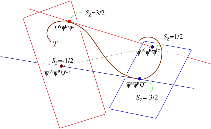
Figure 5: The twisted cubic curve as a system of spin states. The quantum phase space for a spin 3/2 particle contains a preferred twisted cubic ${\cal T}$ which is self-conjugate in the sense that the complex conjugate plane corresponding to any point on ${\cal T}$ necessarily osculates the curve at some other point on ${\cal T}$. The points of ${\cal T}$ are those states which have an eigenstate of spin 3/2 relative to some choice of spin axis. Each point of ${\cal T}$ corresponds to a choice of spin axis and direction.

In order to proceed further, we introduce a spinorial notation and let the symmetric spinor $\psi^{ABC}=\psi^{(ABC)}$ denote homogeneous coordinates on $CP^{3}$. Then, the twisted cubic arising naturally here is determined by the relation

$$\tau_{AB}\ :=\ \psi_{CD(A}\psi^{CD}_{B)}\ =\ 0\ ,$$

where the indices on $\psi^{ABC}$ are raised and lowered according to the standard conventions, so for example, $\psi_{B}^{CD}=\epsilon_{AB}\psi^{ACD}$, and so on. The general solution to the algebraic relations given by $\tau_{AB}=0$ takes the form $\psi^{ABC}=\xi^{A}\xi^{B}\xi^{C}$ for arbitrary $\xi^{A}$ (Hughston, Hurd $\&$ Eastwood 1979).

The specification of a twisted cubic ${\cal T}$ in $CP^{3}$ induces a null polarity on the state space, i.e., a natural correspondence between points and planes such that the polar plane of a given point actually includes that point. The null polarity is given by the map

$$\psi^{ABC}\ \rightarrow\ \psi_{ABC}=\epsilon_{AP}\epsilon_{BQ}\epsilon_{CR}\psi^{PQR}\ ,$$

and it follows as an elementary spinor identity that $\psi^{ABC}\psi_{ABC}=0$ for any choice of $\psi^{ABC}$. In the case of a point $\psi^{ABC}=\xi^{A}\xi^{B}\xi^{C}$ on ${\cal T}$, the corresponding polar plane intersects ${\cal T}$ solely at that point, with a three-fold degeneracy, and is called the osculating plane at that point.

Each choice of $\xi^{A}$, i.e., a point on ${\cal T}$, determines a spin axis. For each spin axis, there are four possible spin eigenstates with eigenvalues $\frac{3}{2}$, $\frac{1}{2}$, $-\frac{1}{2}$, and $-\frac{3}{2}$. Two of the spin states, corresponding to eigenvalues $\pm\frac{3}{2}$, lie on ${\cal T}$ itself. These two states can be written $\psi^{A}\psi^{B}\psi^{C}$ and ${\bar{\psi}}^{A}{\bar{\psi}}^{B}{\bar{\psi}}^{C}$, where ${\bar{\psi}}^{A}=\epsilon^{AB}{\bar{\psi}}_{B}$ and ${\bar{\psi}}_{B}={\bf c}(\psi^{B})$.

The choice of $\psi^{A}$ determines the spin axis. The complex conjugate of the state $\psi^{ABC}=\psi^{A}\psi^{B}\psi^{C}$ on the twisted cubic ${\cal T}$ is the plane ${\bar{\psi}}_{ABC}={\bar{\psi}}_{A}{\bar{\psi}}_{B}{\bar{\psi}}_{C}$ in $CP^{3}$, and this plane is tangent to ${\cal T}$ at the point ${\bar{\psi}}^{A}{\bar{\psi}}^{B}{\bar{\psi}}^{C}$. On the other hand, through the point $\psi^{A}\psi^{B}\psi^{C}$ there is a unique line tangent to ${\cal T}$, and this line intersects the plane ${\bar{\psi}}_{A}{\bar{\psi}}_{B}{\bar{\psi}}_{C}$ at a point, given by $\psi^{(A}\psi^{B}{\bar{\psi}}^{C)}$. This point is the spin $\frac{1}{2}$ eigenstate with respect to that choice of axis. Conversely, the tangent line to ${\cal T}$ at the spin $-\frac{3}{2}$ state ${\bar{\psi}}^{A}{\bar{\psi}}^{B}{\bar{\psi}}^{C}$ intersects the tangent plane of ${\cal T}$ at $\psi^{A}\psi^{B}\psi^{C}$ at the point ${\bar{\psi}}^{(A}{\bar{\psi}}^{B}\psi^{C)}$, which is the spin $-\frac{1}{2}$ state.

An interesting feature of the twisted cubic geometry arises from the fact that for any symmetric spinor $\psi^{ABC}$ we have the relation

$$\tau_{AB}\psi^{ABC}\ =\ 0\ ,$$

which follows from the spinor identity $\epsilon_{[AB}\epsilon_{C]D}=0$. This relation implies that through any point $\psi^{ABC}$ in $CP^{3}-{\cal T}$, i.e., a point off the curve, there exists a unique chord of ${\cal T}$. This follows from the fact that, providing $\tau_{AB}$ is nondegenerate, the condition $\tau_{AB}\psi^{ABC}=0$ implies a relation of the form

$$\psi^{ABC}\ =\ u\xi^{A}\xi^{B}\xi^{C}+v\eta^{A}\eta^{B}\eta^{C}$$

for some $\xi^{A}$ and $\eta^{A}$ corresponding to a pair of spin axes such that $\xi_{A}\eta^{A}\neq 0$, where $(u,v)$ are homogeneous coordinates on $CP^{1}$. It follows that an arbitrary quantum state $\psi^{ABC}$ in $CP^{3}-{\cal T}$ admits a unique characterisation in terms of a superposition of a pair of spin-$\frac{3}{2}$ eigenstates corresponding to distinct spin axes. If $\tau_{AB}$ is degenerate, then the chord reduces to a tangent line to ${\cal T}$ with a double point at the intersection, and $\psi^{ABC}$ has a unique representation of the form $\psi^{ABC}=\xi^{(A}\xi^{B}\eta^{C)}$.

A similar analysis can be pursued in connection with the geometry of a spin-2 system, for which the state space is $CP^{4}$, endowed with a self-conjugate rational quartic curve. The geometry of this curve is closely related to the Petrov-Pirani classification of gravitational fields.

7 Geometry of entanglement

Now consider a more elaborate set-up: the spin degrees of freedom of an entangled pair of spin-$\frac{1}{2}$ particles. The generic two-particle state $\psi^{AB}$ for a pair of such particles (e.g., an electron and a positron) has a 4-dimensional Hilbert space, and the state space is $CP^{3}$. There is a preferred point $Z$ in $CP^{3}$, corresponding to the singlet state of total spin 0, for which $\psi^{AB}=\psi^{[AB]}$. The conjugate plane ${\bar{Z}}$ contains the triplet states of total spin 1, for which $\psi^{AB}=\psi^{(AB)}$. We note that ${\bar{Z}}$ is endowed with a conic ${\cal C}$, each point of which defines a spin axis. There is also a special surface $Q\in CP^{3}$, given by the quadratic equation

$$\epsilon_{AC}\epsilon_{BD}\psi^{AB}\psi^{CD}\ =\ 0\ ,$$

consisting of states of the $disentangled$ form $\psi^{AB}=\xi^{A}\eta^{B}$, representing an embedding of the product of the state spaces of the individual spin-$\frac{1}{2}$ particles. The states off the quadric are the $entangled$ states.

Suppose we start with a combined state of total spin 0 for the two particles, and we measure the spin of the first particle (say, the electron) relative to a given choice of axis. This will disentangle the state, so the result lies on $Q$. The choice of axis and orientation determines a point and its conjugate on the conic ${\cal C}$. The tangents to the conic at these points intersect to form a third point off the quadric but in the plane of total spin 1, corresponding to a triplet state of eigenvalue 0 relative to the axis. We join that state to the starting state $Z$, and the resulting line intersects $Q$ at a pair of points, as shown in Figure 6.

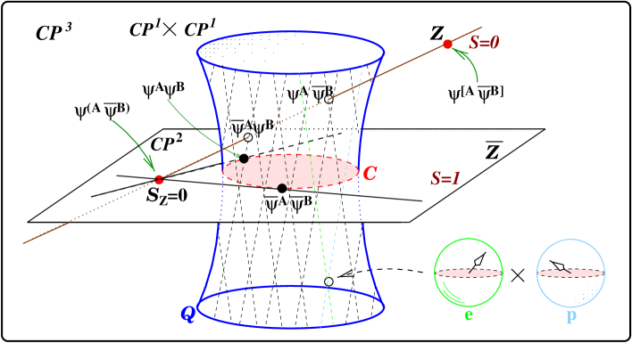
Figure 6: Quantum entanglement. The quantum phase space of an electron-positron system contains a point $Z$ for total spin 0, and a projective hyperplane ${\bar{Z}}$ for total spin 1. The disentangled states have indefinite total spin, and comprise a quadric $Q$ ruled by two systems (electron and positron) of linear generators. Once a spin axis is chosen, the join of $Z$ with the state of total spin 1 and $S_{z}=0$ intersects $Q$ in a pair of points, corresponding to the possible measurement outcomes of the spin of the electron relative to the axis.

The two disentangled states thus obtained represent the possible measurement outcomes. The quadric $Q$ has two systems of generators, corresponding to the electron and positron state spaces. Through each point of $Q$ there is a unique ‘electron generator’ and a unique ‘positron generator’. An electron generator represents a fixed electron state, each point on it corresponding to a possible positron state. The two points constituting the possible outcomes of the spin measurement of the electron have the property that their electron generators hit respectively the two chosen points on the conic that define the spin axis. The measurement result for which the electron generator hits the spin up state on the conic is the ‘electron spin up and positron spin down’ outcome, whereas the other one is the ‘electron spin down and positron spin up’ outcome.

In a more general situation, the idea of quantum entanglement is characterised geometrically by the fact that complex projective space admits a Segre embedding of the form

$$CP^{m}\times CP^{n}\ \hookrightarrow\ CP^{(m+1)(n+1)-1}\ .$$

Here we regard both $CP^{m}$ and $CP^{n}$ as representing the state space of two subsystems, respectively, while $CP^{(m+1)(n+1)-1}$ represents the state space of the combined system. One can argue that this is the main feature of quantum mechanics that has no analogue is classical physics. That is to say, classically, the state space of a combined system is given by the product of the state spaces of the subsystems, which has a moderate dimensionality when compared with the situation of the quantum state space for a combined system.

8 Measure of entanglement

The set up indicated above suggests a methodology according to which a measure $\delta(\psi)$ can be assigned to the degree of entanglement exhibited by a given pure state $\psi$. This is a topic currently of great interest in quantum physics (cf. Linden, et. al. 1999). Let us consider the general case of a finite dimensional two-particle state space $CP^{n}$ containing a subvariety $V^{m}\subset CP^{n}$, where $V^{m}=CP^{j}\times CP^{k}$ and $n=(j+1)(k+1)-1$. The variety $V^{m}$ represents the disentangled states of the two particles, and is given by the product of the respective single particle state space $CP^{j}$ and $CP^{k}$.

We propose, as a measure of entanglement for a generic pure state $\psi\in CP^{n}$, the use of the geodesic distance from the given state $\psi$ to the nearest disentangled state. The distance $\delta$ is measured with respect to the Fubini-Study metric.

Clearly, $\delta$ is a natural measure in the sense that it depends only on the Segre embedding of the variety $V^{m}$ and no additional structure apart from the given metrical geometry of $CP^{n}$. Furthermore, we can demonstrate that $\delta$ is invariant under any unitary transformation of $CP^{n}$ that is also an automorphism of $V^{m}$, i.e., transformations that preserve the disentangled state space. It should be evident that essentially the same construction applies to the case of entangled states of any number of particles. We do not require that the particles are necessarily of the same type.

As a specific illustration, we consider the system described in §7 consisting of two spin-$\frac{1}{2}$ particles, where the state space is $CP^{3}$ and the space $V^{2}$ of disentangled states is a quadric $Q\subset CP^{3}$. Suppose we write $\psi^{AB}$ for a generic state, and $\bar{\psi}_{AB}$ for the corresponding complex conjugate hyperplane. Then the distance $\delta$ from $\psi$ to $Q$ is determined by the relation $\kappa=\frac{1}{2}(1+\cos\delta)$, where $\kappa$ is the cross ratio

$$\kappa\ =\ \frac{(\psi^{AB}{\bar{X}}_{AB})(X^{CD}{\bar{\psi}}_{CD})}{(\psi^{AB}{\bar{\psi}}_{AB})(X^{CD}{\bar{X}}_{CD})},$$

and $X^{AB}\in Q$ maximises $\kappa$ for the given state $\psi^{AB}$. The cross ratio $\kappa$ is the Dirac transition probability from the state $\psi^{AB}$ to the state $X^{AB}$, and our goal is to find the states on $Q$ for which the transition probability from $\psi^{AB}$ is maximal.

We shall turn to the details of the maximisation problem in a moment, in §10, since these are of interest, but here first we present the solution. Let us write $\psi_{CD}:=\epsilon_{AC}\epsilon_{BD}\psi^{AB}$ and ${\bar{\psi}}^{AB}:=\epsilon^{AC}\epsilon^{BD}{\bar{\psi}}_{AB}$, where the antisymmetric spinor $\epsilon_{AB}$ satisfies the usual relation $\epsilon_{AB}\epsilon^{AC}=\delta^{C}_{B}$. Then the solution for $\kappa$ is given by $\kappa=\frac{1}{2}(1+\gamma)$, with

$$\gamma\ =\ \sqrt{1-\frac{(\psi^{AB}\psi_{AB})({\bar{\psi}}^{CD}{\bar{\psi}}_{CD})}{(\psi^{AB}{\bar{\psi}}_{AB})^{2}}}.$$

We note that $\gamma$ is independent of the scale of $\epsilon_{AB}$ and lies in the range $0\leq\gamma\leq 1$. The inequality satisfied by $\gamma$ follows from a general result that for any element ${\bf z}$ in a complex vector space with a Hermitian inner product we have the Hermitian inequality $({\bf z}\cdot{\bar{\bf z}})^{2}\geq({\bf z}\cdot{\bf z})({\bar{\bf z}}\cdot{\bar{\bf z}})$. This can be seen by writing ${\bf z}={\bf a}+{\rm i}{\bf b}$, where ${\bf a}$ and ${\bf b}$ are real, and then checking that the purported relation reduces to the Schwartz inequality $({\bf a}\cdot{\bf b})^{2}\leq({\bf a}\cdot{\bf a})({\bf b}\cdot{\bf b})$.

If the point $\psi^{AB}$ lies on the quadric $Q$, we have $\psi_{AB}\psi^{AB}=0$, and hence $\gamma=1$, which implies $\kappa=1$, from which it follows that the distance to the quadric is $\delta=0$. On the other hand, for a maximally entangled state the inequality is saturated at $\gamma=0$, and thus gives $\kappa=1/2$, which implies $\delta=\pi/2$.

The interpretation of this result is as follows. We recall that for orthogonal states the Fubini-Study distance is $\pi$, the greatest distance possible for two states. On the other hand, the maximum distance an entangled state can have from the closest disentangled state, in the case of two spin-$\frac{1}{2}$ particles, is $\pi/2$. For example, with respect to a given choice of spin axis, the spin 0 singlet state $\epsilon^{AB}$ can be expressed as an antisymmetric superposition of two disentangled states, i.e., an up-down state and a down-up state. The two disentangled states are mutually orthogonal, and the singlet state lies ‘half way’ between them.

9 Hermitian polar conjugation

Now, let us consider the geometry of this situation in more detail. There is a well-known construction in algebraic geometry according to which a proper quadric locus in $CP^{3}$ induces a polarity on this space — a one-to-one correspondence between points and planes. Reverting briefly to the notation of §3, let us write $\psi^{\alpha}$ for the homogeneous coordinates of a point in $CP^{3}$, and $Q_{\alpha\beta}\psi^{\alpha}\psi^{\beta}=0$ for the quadric. We assume that the quadric is nondegenerate, i.e., proper, in the sense that $\det(Q_{\alpha\beta})\neq 0$. Then for any state $\xi^{\alpha}\in CP^{3}$ it follows that ${\tilde{\xi}}_{\alpha}:=Q_{\alpha\beta}\xi^{\beta}$ is nonvanishing. The locus ${\tilde{\xi}}_{\alpha}\psi^{\alpha}=0$ defines the polar plane of the point $\xi^{\alpha}$ with respect to the quadric $Q_{\alpha\beta}$. Since $Q_{\alpha\beta}$ is nondegenerate, there is a unique inverse $Q^{\alpha\beta}$ satisfying $Q_{\alpha\gamma}Q^{\gamma\beta}=\delta_{\alpha}^{\beta}$, and thus for any plane $\eta_{\alpha}$ in $CP^{3}$ we can define a polar point ${\tilde{\eta}}^{\alpha}:=Q^{\alpha\beta}\eta_{\beta}$. The operation is involutory in the sense that the polar point of the polar plane of a given point is that point.

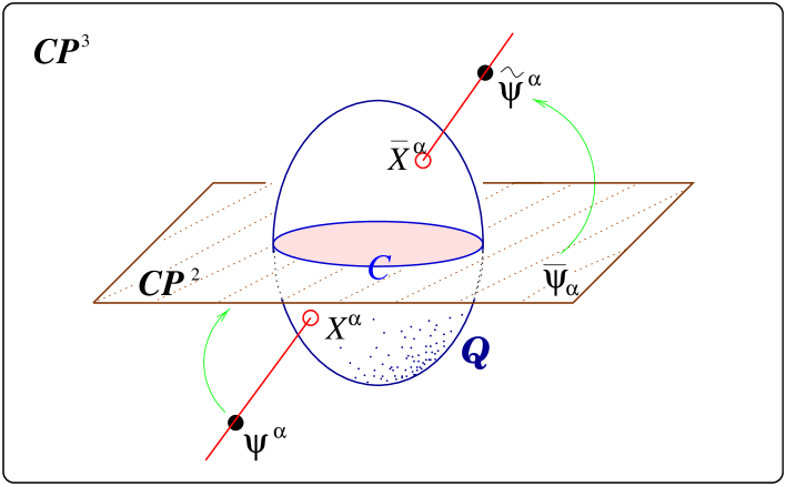
Figure 7: Hermitian polar conjugation and the construction of extremal disentangled states. Given any entangled state $\psi^{\alpha}$ we can form another state ${\tilde{\psi}}^{\alpha}$ given by the harmonic conjugate of the complex conjugate plane of $\psi^{\alpha}$ with respect to the quadric $Q$. The points on $Q$ nearest to and furthest from $\psi^{\alpha}$ are given by the intersection points $X^{\alpha}$ and ${\bar{X}}^{\alpha}$ of $Q$ with the line joining $\psi^{\alpha}$ and ${\tilde{\psi}}^{\alpha}$.

One way of constructing the polar plane of a point $\xi$ is as follows. Let $L$ be an arbitrary line $L^{\alpha\beta}=\xi^{[\alpha}\zeta^{\beta]}$ through $\xi$. Then $L$ intersects $Q$ twice, say, at points $A$ and $B$. Now suppose we consider the harmonic conjugate $\xi^{*}$ of $\xi$, on the line $L$, with respect to the points $A$ and $B$. This is the unique point $\xi^{*}$ on $L$ such that we have

$$\{\xi,\xi^{*};A,B\}\ =\ -1$$

for the cross ratio. Then, as we vary $L$, the locus of $\xi^{*}$ sweeps out a plane, and this is the polar plane ${\tilde{\xi}}$. The polar plane ${\tilde{\xi}}$ intersects $Q$ in a conic ${\cal C}$ with the property that any line drawn from $\xi$ to ${\cal C}$ touches $Q$ tangentially.

Conversely, if we consider all the lines through $\xi$ that touch $Q$ tangentially, then the union of the intersection points is the conic ${\cal C}$, which lies in a unique plane, the polar plane ${\tilde{\xi}}$. A point lies on its polar plane iff the point itself lies on the quadric, in which case the polar plane of the point is the tangent plane at that point. In that case, the conic ${\cal C}$ degenerates into a pair of lines, given by the two generators of the quadric through the given point.

In the quantum mechanical situation we require further that the quadric $Q_{\alpha\beta}$ be Hermitian in the sense that $Q_{\alpha\beta}={\bar{Q}}_{\alpha\beta}$ and $Q^{\alpha\beta}={\bar{Q}}^{\alpha\beta}$. This ensures that the complex conjugate ket-vector $|{\bar{\tilde{x}}}\rangle$ of the polar bra-vector $\langle{\tilde{x}}|$ of a given ket-vector $|x\rangle$ agrees with the polar ket-vector $|{\tilde{\bar{x}}}\rangle$ of the complex conjugate bra-vector $\langle{\bar{x}}|$ of the given ket-vector $|x\rangle$. It follows that complex conjugate ket-vector of the polar bra-vector of a disentangled state is also disentangled, and that the polar ket-vector of the complex conjugate bra-vector of a disentangled state is disentangled.

The situation described so far applies to the consideration of any pair of two-state systems, whether or not these systems are of the same type. For example, we might consider a simple toy model in which a lepton is regarded as a composite consisting of a neutral spin-$\frac{1}{2}$ particle and a spin-0 flavour doublet that determines whether the lepton is an electron or a muon. Then one might explore the properties of the entangled state given by a superposition of a spin-up electron with a spin-down muon, the spin state being given with respect to some choice of axis. What distinguishes the state space of a pair of spin-$\frac{1}{2}$ particles is the existence of a preferred singlet state $Z^{\alpha}$. This state is required to be self-conjugate polar with respect to the quadric in the sense that ${\bar{Z}}_{\alpha}=Q_{\alpha\beta}Z^{\beta}$.

10 Maximal entanglement

We are now in a position to present a more geometrical construction for the supremum of the cross-ratio $\kappa$ under the given constraint. Given the entangled state $\psi^{\alpha}$ we wish to find the state $X^{\alpha}\in Q$ that maximises the cross ratio

$$\kappa\ =\ \frac{(\psi^{\alpha}{\bar{X}}_{\alpha})(X^{\beta}{\bar{\psi}}_{\beta})}{(\psi^{\alpha}{\bar{\psi}}_{\alpha})(X^{\beta}{\bar{X}}_{\beta})}.$$

In fact, suppose we define ${\bar{\psi}}^{\alpha}:=Q^{\alpha\beta}{\bar{\psi}}_{\beta}$, the polar state of the complex conjugate hyperplane ${\bar{\psi}}_{\alpha}$. Then we can show that the states on $Q$ that are maximally and minimally distant to the given state $\psi^{\alpha}$ are collinear with $\psi^{\alpha}$, and are complex conjugate polar to one another in the sense that $\psi^{\alpha}$ has to be of the form

$$\psi^{\alpha}\ =\ pX^{\alpha}+qQ^{\alpha\beta}{\bar{X}}_{\beta}$$

where $X^{\alpha}$ is the point on $Q$ closest to $\psi^{\alpha}$, so $|p|\geq|q|$. This can be verified, for example, by maximising $\kappa$ with respect to $X^{\alpha}$ subject to the constraint $Q_{\alpha\beta}X^{\alpha}X^{\beta}=0$, using a Lagrange multiplier technique. Then if we define $\lambda=p/q$ it follows by a direct substitution that

$$\kappa\ =\ \frac{\lambda{\bar{\lambda}}}{1+\lambda{\bar{\lambda}}}.$$

Since $\lambda{\bar{\lambda}}\geq 1$, it follows, further, that $\frac{1}{2}\leq\kappa\leq 1$. On the other hand, we can also verify by direct substitution that the invariant $\rho$ defined by

$$\rho\ =\ \frac{(Q_{\alpha\beta}\psi^{\alpha}\psi^{\beta})({\bar{Q}}^{\gamma\delta}{\bar{\psi}}_{\gamma}{\bar{\psi}}_{\delta})}{(\psi^{\gamma}{\bar{\psi}}_{\gamma})^{2}},$$

which is independent of the scale of $Q_{\alpha\beta}$, depends on $p$ and $q$ only through $\lambda$, and is given by the formula

$$\rho\ =\ \frac{4\lambda{\bar{\lambda}}}{(1+\lambda{\bar{\lambda}})^{2}}.$$

Then it is not difficult to see that $\kappa$ is indeed of the desired form $\kappa=\frac{1}{2}(1+\gamma)$ with

$$\gamma\ =\ \sqrt{1-\rho}.$$

That establishes the the validity of the expression indicated earlier for the minimum distance

$$\delta\ =\ \cos^{-1}\sqrt{1-\rho}$$

from the given state $\psi^{\alpha}$ to the quadric of disentanglement.

The maximally entangled states are those for which $|\lambda|=1$, for which apart from an overall irrelevant scale factor $\psi^{\alpha}$ is thus necessarily of the form

$$\psi^{\alpha}\ =\ e^{{\rm i}\theta}X^{\alpha}+e^{-{\rm i}\theta}Q^{\alpha\beta}{\bar{X}}_{\beta}.$$

Such states are self-conjugate in the sense that ${\bar{\psi}}_{\alpha}=Q_{\alpha\beta}\psi^{\beta}$. Conversely, given any disentangled state $X^{\alpha}$ we see that there exists a one-parameter family of maximally entangled states at a distance $\pi/2$ from it. This one-parameter family is given by the equatorial circle of the complex projective line obtained by joining $X^{\alpha}$ to the conjugate entangled state $Q^{\alpha\beta}{\bar{X}}_{\beta}$, to which $X^{\alpha}$ is orthogonal.

Thus, for example, if $X^{AB}=\xi^{A}\eta^{B}$ is a disentangled state of two spin-$\frac{1}{2}$ particles, then we obtain the one-parameter family of maximally entangled states given by $\psi^{AB}=e^{{\rm i}\theta}\xi^{A}\eta^{B}+e^{-{\rm i}\theta}{\bar{\xi}}^{A}{\bar{\eta}}^{B}$ where ${\bar{\xi}}^{A}:=\epsilon^{AB}{\bar{\xi}}_{B}$ and ${\bar{\eta}}^{B}:=\epsilon^{BA}{\bar{\eta}}_{A}$. For any value of $\theta$ these states are at a distance of $\pi/2$ from $X^{AB}$.

A special case of interest arises when $\eta^{B}={\bar{\xi}}^{B}$ and ${\bar{\eta}}^{A}=-\xi^{A}$. In that case, reverting to the notation of the previous section, we have $\psi^{AB}=e^{{\rm i}\theta}\psi^{A}{\bar{\psi}}^{B}-e^{-{\rm i}\theta}{\bar{\psi}}^{A}\psi^{B}$. Then for $\theta=0$ we obtain the spin 0 singlet state for which $\psi^{AB}\propto\epsilon^{AB}$; whereas for $\theta=\pi$ we get the $S_{z}=0$ spin 1 triplet state for which $\psi^{AB}\propto\psi^{(A}{\bar{\psi}}^{B)}$.

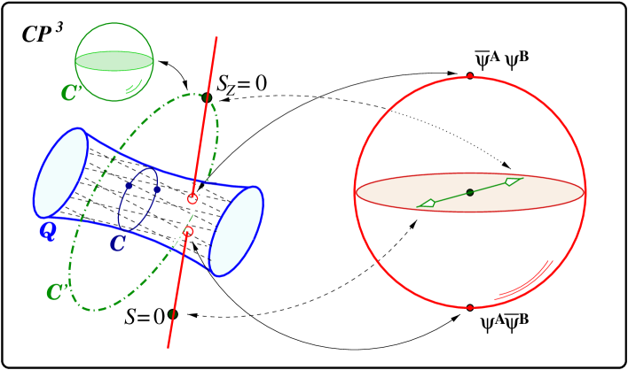
Figure 8: Maximally entangled states. Through any conjugate pair of disentangled states on $Q$ there exists a complex projective line containing the $S=0$ singlet and an $S_{z}=0$ triplet state for some choice of $z$-axis. The singlet and triplet states lie on an equatorial circle at a distance of $\pi/2$ from the disentangled states which are orthogonal to one another and thus lie on opposite poles. All the points on this equatorial circle are maximally entangled. The trajectory of the entangled triplet states corresponding to different spatial directions is a conic $C^{\prime}$, which has a topology of a sphere. Hence the space of maximally entangled states has the structure of $S^{2}\times S^{1}$.

More generally, if $\psi^{\alpha}$ is an arbitrary maximally entangled state, then consider the conic ${\cal K}$ that arises when we intersect the plane ${\bar{\psi}}_{\alpha}$ with the quadric $Q$. This conic is conjugate self-polar in the sense that for any point $\pi^{\alpha}$ on ${\cal K}$ the complex conjugate plane ${\bar{\pi}}_{\alpha}$ is tangent to the quadric at a point ${\bar{\pi}}^{\alpha}$ on ${\cal K}$. Now, suppose we consider the locus ${\cal L}$ of points generated by the intersection of the tangent lines to $\pi^{\alpha}$ and ${\bar{\pi}}^{\alpha}$ in the plane ${\bar{\psi}}_{\alpha}$ as we vary $\pi^{\alpha}$. For any point $P$ in ${\cal L}$ the join of that point with $\psi^{\alpha}$ intersects $Q$ in a pair of points $X^{\alpha}$ and ${\bar{X}}^{\alpha}$, both of which are at a distance $\delta=\pi/2$. By varying $P$ we obtain all points on $Q$ at a distance $\pi/2$ from $\psi^{\alpha}$.

Finally, let us consider the case of sub-maximally entangled states. In this situation the relation between $\psi^{\alpha}$ and $X^{\alpha}$ is invertible, since providing $|\lambda|>1$ there exist complex numbers $r$ and $s$ such that

$$X^{\alpha}\ =\ r\psi^{\alpha}+sQ^{\alpha\beta}{\bar{\psi}}_{\beta}.$$

We can solve this for the ratio $\mu=r/s$ by imposing the condition $Q_{\alpha\beta}X^{\alpha}X^{\beta}=0$, leading to the quadratic equation $\mu^{2}Q_{\alpha\beta}\psi^{\alpha}\psi^{\beta}+2\mu\psi^{\alpha}{\bar{\psi}}_{\alpha}+{\bar{Q}}^{\alpha\beta}{\bar{\psi}}_{\alpha}{\bar{\psi}}_{\beta}=0$, for which the roots are given by

$$\mu\ =\ \frac{-1\pm\sqrt{1-q{\bar{q}}}}{q},$$

where $q:=Q_{\alpha\beta}\psi^{\alpha}\psi^{\beta}/\psi^{\gamma}{\bar{\psi}}_{\gamma}$. The positive root gives the point on $Q$ nearest to $\psi$, and the negative root gives the most distant disentangled state. We note that the terms here are so constructed that the solution for $X^{\alpha}$ is independent of the overall scale and phase of $\psi^{\alpha}$, as expected.

11 Schrödinger evolution

As the examples above indicate, the geometry of quantum mechanics is very rich, once specific physical systems are brought into play, even when there are only a few degrees of freedom. This picture can be further developed by consideration of the dynamics of a quantum system, which can be pictured as a vector field on the state manifold. Such a vector field generates a symmetry of the Fubini-Study geometry, i.e., an action of the projective unitary group.

In the case of an $(n+1)$-dimensional Hilbert space, the state space is $CP^{n}$, which can be viewed as a real manifold ${\sl\Gamma}$ of dimension $2n$, with a symmetry group of dimension $n(n+2)$, generated by a family of $n(n+2)$ Killing vector fields. A generic Killing field on ${\sl\Gamma}$ has $n+1$ fixed points, corresponding to eigenstates of the given Hamiltonian.

In the case of a 2-dimensional Hilbert space, the state space is $CP^{1}$, and the specification of a Killing field selects out a pair of polar points on $S^{2}$, corresponding to energy eigenstates $E_{1}$ and $E_{2}$. The relevant symmetry is then given by a rigid rotational flow about this axis, the angular frequency being determined by Planck’s formula $E_{2}-E_{1}=\hbar\omega$. In the case of the state space $CP^{n}$, the $n+1$ fixed points of a given Killing field are linked by a figure consisting of $\frac{1}{2}n(n+1)$ spheres, for which the fixed points act as polar points, in pairs. These spheres rotate respectively with angular frequencies

$$E_{i}-E_{j}\ =\ \hbar\omega_{ij}\ ,$$

where $E_{i}$ ($i=1,2,\cdots,n+1$) labels the energy of $i$th eigenstate. The dynamical trajectories in ${\sl\Gamma}$ are determined by the specification of the fixed points, along with the associated angular frequencies. Even in the case of a simple spin 1 system, the geometry of the state space is intricate, given by a 4-dimensional manifold containing three 2-spheres touching one another at the poles, and spinning at three distinct frequencies.

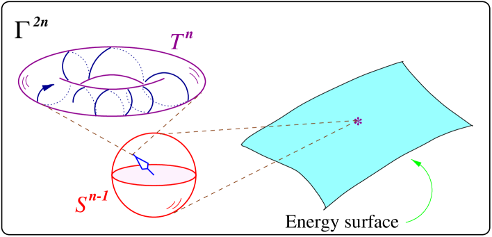
Figure 9: Foliation of the state space and quantum dynamical trajectories. The quantum state space is foliated by level surfaces of the expectation of the Hamiltonian operator. Each point on such a surface is parameterised by a family of $n$ phase variables, $n-1$ angular coordinates, and one energy variable. The Schrödinger evolution preserves the energy and the angular coordinates of a given initial state (point), and the resulting dynamical trajectory is thus confined to the $n$-torus $T^{n}$. If the ratios $E_{i}/E_{j}$ of the energy eigenvalues are irrational, then the trajectory on $T^{n}$ does not close.

If the frequencies are not commensurate in the sense of being rational multiples of each other, then the Killing orbits do not close except on the three special spheres, and the generic dynamical trajectory, starting from some initial point in the state space, is doomed to evolve to eternity without ever returning to its origin. More specifically, we can view the quantum state space $CP^{n}$ as a real manifold ${\sl\Gamma}^{2n}$ of dimension $2n$. Then, we can consider a foliation of ${\sl\Gamma}^{2n}$ by level surfaces of constant energies. The specification of the energy thus determines one of the $2n$ real coordinates on the state space. The remaining $2n-1$ coordinates can be identified (Brody $\&$ Hughston 1999b) with $n-1$ angular coordinates and $n$ phase variables. In other words, each energy surface has the structure of a product space of an $n$-torus and an ($n-1$)-sphere, i.e., $T^{n}\times S^{n-1}$. Given an initial point on one of the energy surfaces, the dynamics induced by the Schrödinger evolution will confine that point to the torus that contains the initial state. In other words, the angular variables of the initial state remain unchanged under the action of the projective unitary group induced by the given quantum Hamiltonian. It follows, therefore, that the Schrödinger evolution is at best merely quasiergodic on the energy surface.

12 Quantum Hamiltonian dynamics

This line of argument can be taken further by studying the quantum trajectories on ${\sl\Gamma}$ by use of differential geometry. When viewed as a real manifold, the state space is endowed with a Riemannian structure, given by a positive definite symmetric metric $g_{ab}$, a symplectic structure, given by an antisymmetric tensor $\Omega_{ab}$, and a complex structure, given by a tensor $J^{a}_{\ b}$, satisfying

$$J^{a}_{\ c}J^{c}_{\ b}\ =\ -\delta^{a}_{\ b}\ .$$

These structures are required to be compatible in the sense that $\Omega_{ab}=g_{ac}J^{c}_{\ b}$ and $\nabla_{a}J^{b}_{\ c}=0$, where $\nabla_{a}$ is the covariant derivative associated with $g_{ab}$. Here we use Roman indices ($a,b,\cdots$) for tensorial operations in the tangent space of ${\sl\Gamma}$. The compatibility of $g_{ab}$, $\Omega_{ab}$, and $J^{a}_{\ b}$ makes ${\sl\Gamma}$ a Kähler manifold. For some purposes it suffices to assume that the metric $g_{ab}$ and the symplectic structure $\Omega_{ab}$ are only weakly nondegenerate in the sense that for any vector fields $\xi^{a},\eta^{a}$ on ${\sl\Gamma}$, $\xi^{a}g_{ab}=0$ implies $\xi^{a}=0$ and $\eta^{a}\Omega_{ab}=0$ implies $\eta^{a}=0$. The fact that in infinite dimensions the Fubini-Study metric and symplectic structure are strongly nondegenerate (Marsden $\&$ Ratiu 1999) means that many of the geometrical constructions carried out in finite dimensions carry through to the general quantum phase space.

The additional ingredient required for the specification of the dynamics is a Hamiltonian function $H(x)$ on ${\sl\Gamma}$. Then the general dynamical trajectories on ${\sl\Gamma}$ are given by

$$\frac{1}{2}\hbar\Omega_{ab}dx^{b}\ =\ \nabla_{a}Hdt\ .$$

The Schrödinger trajectories on ${\sl\Gamma}$ are given by a subclass of the general Hamiltonian trajectories, namely, those for which the Hamiltonian function $H(x)$ is of the special form

$$H(x)\ =\ \frac{{\bar{\psi}}_{\alpha}(x)H^{\alpha}_{\beta}\psi^{\beta}(x)}{{\bar{\psi}}_{\gamma}(x)\psi^{\gamma}(x)}\ .$$

Here, $\psi^{\alpha}(x)$ denote homogeneous coordinates for the corresponding point $x$ in the projective Hilbert space. Thus for a Schrödinger trajectory, $H(x)$ is the expectation of the Hamiltonian operator in the pure state to which the point $x$ corresponds. In contrast with classical mechanics, where the phase space often has an interpretation in terms of position and momentum variables, in quantum mechanics the points in phase space correspond to pure quantum states.

Quantum observables are intimately related to the metrical geometry of ${\sl\Gamma}$. The distinguishing feature of a quantum Hamiltonian function $H(x)$ is that the associated symplectic gradient flow $\xi^{a}=dx^{a}/dt$ is a Killing field, i.e., $\nabla_{(a}\xi_{b)}=0$. Indeed all Killing fields on ${\sl\Gamma}$ arise in this way through quantum observables. The Killing fields generate the symmetries of the Fubini-Study metric $g_{ab}$.

In the case of finite dimensions, we can say more about the quantum observables that generate isometries on the Fubini-Study manifold. If $H(x)$ is a linear observable function, then in finite dimensions it is necessarily defined globally on ${\sl\Gamma}$. In fact, one can show that such functions correspond to global solutions of the characteristic equation

$$\nabla^{2}H\ =\ (n+1)({\bar{H}}-H)\ ,$$

where $\nabla^{2}$ is the Laplace-Beltrami operator on ${\sl\Gamma}$, ${\bar{H}}=H^{\alpha}_{\alpha}/(n+1)$ is the uniform average of the eigenvalues of $H^{\alpha}_{\beta}$, and $2n$ is the real dimension of ${\sl\Gamma}$. Conversely, if we are given a Killing field $\xi^{a}$, the corresponding observable function $H(x)$ can be recovered, up to an additive constant, via the relation

$$\hbar\Omega^{ab}\nabla_{a}\xi_{b}\ =\ 2(n+1)(H-{\bar{H}})\ ,$$

which follows directly from the characteristic equation if we make use of the fact that $\hbar\xi_{a}=2J^{b}_{\ a}\nabla_{b}H$. We note, incidentally, that in the Kibble-Weinberg theory, a general nonlinear quantum observable is a function on ${\sl\Gamma}$ such that the characteristic equation is not satisfied. As a consequence, the corresponding symplectic gradient flow is no longer a Killing field.

13 Uncertainty relations

The metrical geometry of ${\sl\Gamma}$ also determines the statistical properties of observables. For example, in the pure state $x$ the squared uncertainty (variance) of an observable represented by the function $F(x)$ is $(\Delta F)^{2}=g_{ab}F^{a}F^{b}$ where $F^{a}$ is the unique gradient vector field satisfying $g_{ab}F^{b}=\nabla_{a}F$. This leads to the following interpretation of quantum mechanical uncertainty. We foliate ${\sl\Gamma}$ with surfaces given by level values of $F(x)$. Through a given pure state $x$ there is a unique such surface, and the uncertainty $\Delta F$ is the length of the gradient vector to that surface at $x$. The observables $F(x)$ and $G(x)$ are incompatible if their Poisson bracket $[F,G]=\Omega_{ab}F^{a}G^{b}$ is nonvanishing. In that case the Heisenberg uncertainty relation

$$(\Delta F)^{2}(\Delta G)^{2}\ \geq\ \frac{1}{4}\left|[F,G]\right|^{2}$$

follows directly as a consequence of the geometric inequality

$$(g_{ab}F^{a}F^{b})(g_{ab}G^{a}G^{b})\ \geq\ (g_{ab}F^{a}G^{b})^{2}+\frac{1}{4}(\Omega_{ab}F^{a}G^{b})^{2}\ ,$$

if we omit the first term in the right hand side. This inequality holds for any vector fields $F^{a}$ and $G^{a}$ on a Kähler manifold. Note that the omitted term $g_{ab}F^{a}G^{b}$ gives rise to the anticommutator of the observables $F$ and $G$.

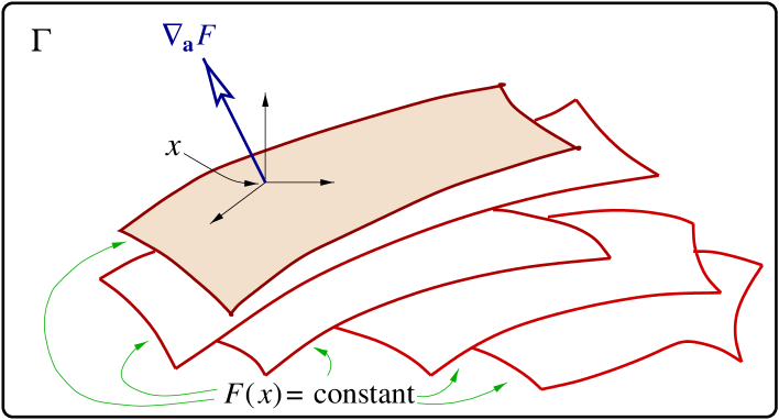
Figure 10: The observable uncertainty. The quantum phase space ${\sl\Gamma}$ is foliated by level surface of the function $F(x)$. The quantum uncertainty in the corresponding observable, in the pure state $x$, is given by the magnitude of the gradient of $F(x)$ at that point.

In the case of a pair of canonically conjugate observables $P(x)$ and $Q(x)$ satisfying $[P,Q]=\hbar$, we can expand the gradient to the surfaces of constant $Q(x)$ in a suitable basis to obtain a series of generalised Heisenberg relations (Brody $\&$ Hughston 1996, 1997, 1998a,b), an example of which is

$$(\Delta P)^{2}(\Delta Q)^{2}\ \geq\ \frac{1}{4}\hbar^{2}\left(1+\frac{(\mu_{4}(P)-3\mu_{2}(P)^{2})^{2}}{\mu_{6}(P)\mu_{2}(P)-\mu_{4}(P)^{2}}\right)\ ,$$

where $\mu_{k}(P)=\langle(P-\langle P\rangle)^{k}\rangle$ is the $k$th central moment of the observable $P$ in the state $x$. This inequality has the following statistical interpretation. Suppose that we are given an unknown quantum state of a particle, parameterised by its position $q$, and that we wish to estimate the position of the particle by a suitable measurement. The observable function corresponding to the parameter $q$ is then given by $Q$, and the statistical estimation of $q$ via measurement on $Q$ gives rise to an inevitable variance lower bound, expressed in terms of a certain combination of the moments $\mu_{k}(P)$ of the momentum distribution associated with the given state. Likewise, if we consider momentum estimation, then the corresponding variance lower bound is given by the moments of the position $Q$.

14 Geometric phases

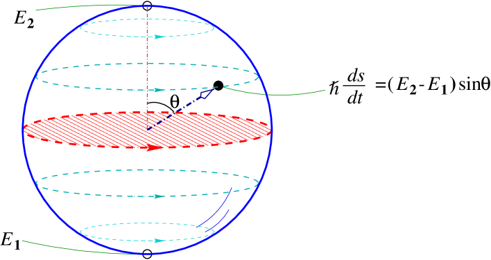
Figure 11: The Anandan-Aharonov relation. The quantum evolution of a 2-state system corresponds to the rigid rotation of a 2-sphere with angular frequency $\hbar\omega=E_{2}-E_{1}$. The speed of the trajectory is greatest at the equator, which consists of states of maximal energy uncertainty.

An interesting interplay between the quantum dynamical trajectories and the uncertainty relations was pointed out by Aharonov $\&$ Anandan (1990). In particular, it follows from the projective Schrödinger equation $\hbar\Omega_{ab}dx^{b}=2\nabla_{a}Hdt$ and the expression for the line element $ds^{2}=g_{ab}dx^{a}dx^{b}$ that the ‘speed’ in the state space ${\sl\Gamma}$ along the dynamical trajectory at the point $x$ is given by

$$\hbar\frac{ds}{dt}\ =\ 2\Delta H\ ,$$

where $\Delta H$ is the energy uncertainty in the given state. For example, in the case of a 2-state system with eigenstates at the poles of a 2-sphere, the quantum evolution corresponds to a rigid rotation of the sphere, with constant angular frequency, for which the speed is greatest at the equator, corresponding to states of maximum uncertainty.

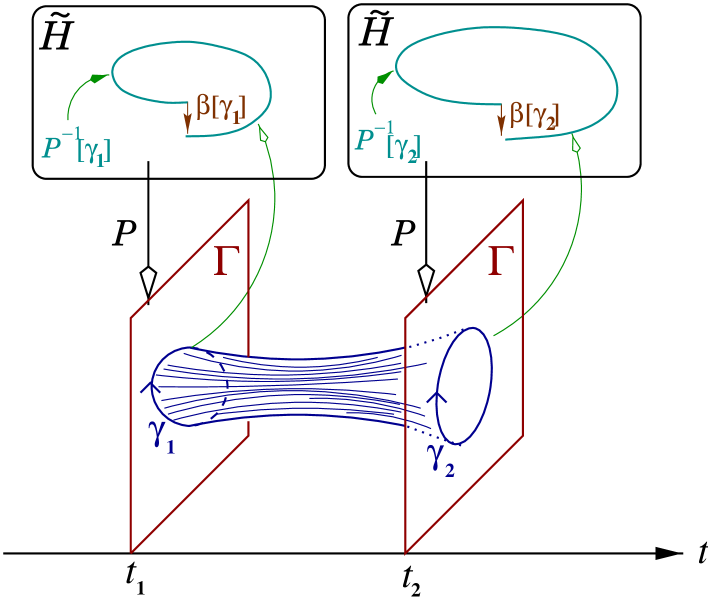
Figure 12: The horizontal lift of a quantum trajectory and Poincare’s invariant integral. The Berry phase $\beta[\gamma]$ associated with a general cyclic trajectory $\gamma$ in the quantum phase space ${\sl\Gamma}$ is given by the integral of the symplectic form $\Omega_{ab}$ over a 2-surface $\Sigma$ spanning $\gamma$. This integral measures the phase change that develops in the horizontal lift of $\gamma$ to the corresponding path ${\cal P}^{-1}[\gamma]$ in the Hilbert bundle ${\tilde{\cal H}}$ over ${\sl\Gamma}$. If the cyclic trajectory subsequently evolves unitarily in time, then $\beta[\gamma]$ is the quantum mechanical integral invariant of Poincare. As a consequence, we have $\beta[\gamma_{1}]=\beta[\gamma_{2}]$. This result is valid even if we relax the unitarity condition and consider nonlinear dynamics of the Kibble-Weinberg type.

This result is related to properties of the geometric phase introduced by Berry and subsequently applied in many situations (Simon 1983; Berry 1984; Uhlmann 1986, see also Shapere $\&$ Wilczek 1989). Consider a closed path $\gamma$ in the quantum phase space. If $\gamma$ is a standard dynamical trajectory, then it corresponds to a closed Killing orbit, but we shall allow for the possibility of more general paths, e.g., as might be generated by a time-dependent Hamiltonian operator. The geometric phase associated with such a cyclic evolution is given by

$$\beta[\gamma]\ =\ \int_{\Sigma}\Omega_{ab}dx^{a}\wedge dx^{b}\ ,$$

where $\Sigma$ is any real 2-surface in ${\sl\Gamma}$ such that $\gamma=\partial\Sigma$. Owing to the relation $\nabla_{a}\Omega_{bc}=0$, it follows from Stokes’ theorem that the value of $\beta[\gamma]$ is independent of the choice of surface $\Sigma$ spanning the loop $\gamma$, and can be given the following interpretation.

The punctured Hilbert space ${\tilde{\cal H}}={\cal H}-\{0\}$, obtained by deleting the origin, is a fibre bundle over ${\sl\Gamma}$. Therefore, given a trajectory $\gamma$ in ${\sl\Gamma}$, we can form a corresponding trajectory ${\cal P}^{-1}[\gamma]$ in ${\tilde{\cal H}}$, called horizontal lift of $\gamma$. This is obtained by solving the modified Schrödinger equation

$${\rm i}\hbar\frac{\partial\psi^{\alpha}}{\partial t}\ =\ (H^{\alpha}_{\beta}-{\rm E}[H]\delta^{\alpha}_{\beta})\psi^{\beta},$$

where ${\rm E}[H]$ is the expectation of the Hamiltonian in the state $\psi^{\alpha}$. Despite its nonlinearity, the modified Schrödinger equation is physically natural inasmuch as its stationary states are energy eigenstates. In this connection, it is worth drawing attention to the fact that in the case of the modified Schrödinger dynamics, the time independent Schrödinger equation

$$H^{\alpha}_{\beta}\psi^{\beta}\ =\ {\rm E}[H]\psi^{\alpha}$$

follows directly from the stationary state requirement, without the introduction of the so-called correspondence principle ${\rm E}[H]\leftrightarrow{\rm i}\hbar\partial_{t}$.

The horizontal lift is characterised by the condition that the tangent to the curve ${\cal P}^{-1}[\gamma]$ in ${\tilde{\cal H}}$, given by $\partial\psi^{\alpha}/\partial t$, is orthogonal to the fibre direction $\psi^{\alpha}$, so we have ${\bar{\psi}}_{\alpha}\partial\psi^{\alpha}/\partial t=0$.

In the case of a closed loop $\gamma$, $\beta[\gamma]$ measures the phase change in $\psi^{\alpha}$ over the corresponding circuit in ${\cal P}^{-1}[\gamma]$. If the given loop $\gamma$ in ${\sl\Gamma}$ subsequently evolves in time, then $\beta[\gamma]$ is a quantum mechanical analogue of the Poincare integral invariant (cf. Arnold 1989). We note, incidentally, that the notion of geometric phase discussed here also applies to nonlinear quantum mechanics, for which the Hamiltonian $H(x)$ does not satisfy the characteristic equation for linear observables.

15 Mixed states

Phase space geometry sheds some interesting light on the role of probability in quantum mechanics. There are at least two situations where probability distributions on the state manifold ${\sl\Gamma}$ have to be considered. One is in the description of the statistical properties of a measurement outcome; the other is in quantum statistical mechanics.

In both cases, the state of the system can be characterised by a probability density function $\rho(x)$ on ${\sl\Gamma}$, in terms of which the expectation of any function $F(x)$ on ${\sl\Gamma}$ can be written

$${\rm E}[F]\ =\ \int_{\sl\Gamma}\rho(x)F(x)dx.$$

We think of $F(x)$ as representing the expectation of the corresponding observable, conditional on the pure state $x$. Then ${\rm E}[F]$ is the unconditional expectation, where we average $F(x)$ over the pure states, weighting with the density $\rho(x)$. A pure state arises if $\rho(x)$ is a $\delta$-function concentrated on a point in ${\sl\Gamma}$. Consider the example of a measurement where initially the system is in a pure state $X$, and the observable has a finite number of eigenstates, as in the case of a spin-1 system when we measure the spin along an axis. The result of this measurement is one of the three spin eigenstates, and these arise with probabilities determined by the Fubini-Study distance. Thus the density function $\rho(x)$ for the state of the system after a measurement is given by a sum of three $\delta$-functions, concentrated at the eigenstates, weighted by these probabilities.

In the case of a quantum observable, the unconditional variance of $F(x)$ in a general mixed state $\rho(x)$ is given by

$${\rm V}[F]\ =\ \int_{\sl\Gamma}\rho(x)(F(x)-{\rm E}[F])^{2}dx+\int_{\sl\Gamma}\rho(x)(g_{ab}F^{a}F^{b})^{2}dx\ .$$

A further simplification emerges by virtue of the special form of a linear observable, for which we have ${\rm E}[F]=\rho^{\alpha}_{\beta}F^{\beta}_{\alpha}$, where

$$\rho^{\alpha}_{\beta}\ =\ \int_{\sl\Gamma}\rho(x)\frac{{\bar{\psi}}_{\beta}(x)\psi^{\alpha}(x)}{{\bar{\psi}}_{\gamma}(x)\psi^{\gamma}(x)}dx$$

is the density matrix associated with $\rho(x)$. For ordinary linear quantum mechanics it suffices to consider the density matrix alone, since all statistical quantities calculated with $\rho(x)$ reduce to expressions involving $\rho^{\alpha}_{\beta}$. Therefore, for certain purposes we can regard $\rho^{\alpha}_{\beta}$ itself as representing the state of the system.

One should bear in mind, however, that the density matrix $\rho^{\alpha}_{\beta}$, which is the lowest moment of the projection operator in the state $\rho(x)$, does not in general contain all the information of the system when we are dealing with nonlinear observables. This follows from the fact that the information of a generic state $\rho(x)$ is contained in the set of all the moments (cf. Brody $\&$ Hughston 1999c). More specifically, in the case of a nonlinear observable, we must consider a general state $\rho(x)$, pure or mixed, because the density matrix is not sufficient to take the expectation of such an observable. Some specific examples of nonlinear observables have been studied by Weinberg (1989a,b). The entanglement measure $\delta$ introduced in §8 provides another explicit example of a nonlinear observable arising in a natural context. Exclusive consideration of the density matrix in a nonlinear setting can lead to paradoxical and apparently nonphysical conclusions, such as the possibility of superluminal EPR communication (cf. Gisin 1989; Polchinski 1991).

Given a general state $\rho(x)$ and a Hamiltonian $H(x)$, the evolution of $\rho(x)$ is governed by the Liouville equation,

$$\frac{1}{2}\hbar{\dot{\rho}}(x)\ =\ \Omega^{ab}\nabla_{a}\rho\nabla_{b}H\ ,$$

where the Poisson bracket between $\rho(x)$ and $H(x)$ is determined by the symplectic structure $\Omega_{ab}$ on ${\sl\Gamma}$. In the case where the Hamiltonian is a linear quantum observable, the Liouville equation is equivalent to the standard Schrödinger dynamics associated with a mixed state $\rho(x)$. On the other hand, if the Hamiltonian is a nonlinear observable, then the Liouville equation no longer corresponds to a linear Schrödinger evolution.

It is interesting to note, nevertheless, that, contrary to what has been argued in literature (cf. Peres 1989), in the case of nonlinear quantum mechanics of the Kibble-Weinberg type, the quantum entropy

$$S(\rho)\ =\ -\int_{\sl\Gamma}\rho(x)\ln\rho(x)dx$$

associated with a general mixed state $\rho(x)$ remains constant in time. This follows as a direct consequence of the Liouville equation for $\rho(x)$.

More generally, the definition of entropy and equilibrium in quantum statistical mechanics brings up important conceptual issues, since, like the quantum measurement problem, it involves the interface of microscopic and macroscopic physics. There is also a profound relationship to fundamental issues in probability theory. Suppose we consider a quantum system characterised by a state space ${\sl\Gamma}$ and a Hamiltonian function $H(x)$ with discrete, possibly degenerate energy levels $E_{j}$ $(j=1,2,\cdots,N)$. Let us write $\delta_{j}(x)$ for a normalised $\delta$-function on ${\sl\Gamma}$ concentrated on the pure state $x_{j}$ with energy $E_{j}$. Thus, $x_{j}$ is the $j$th energy eigenstate. Then if the quantum system is in equilibrium with a heat-bath at inverse temperature $\beta=1/kT$, the state of the system is

$$\rho(x)\ =\ \frac{\sum_{j}\exp(-\beta E_{j})\delta_{j}(x)}{Z(\beta)}\ ,$$

where $Z(\beta)=\sum_{j}\exp(-\beta E_{j})$ is the partition function. This is the canonical distribution of quantum statistical mechanics, characterised by a Gibbs distribution concentrated on the energy eigenstates with Boltzmann weights $\exp(-\beta E_{j})/Z(\beta)$. The standard canonical density matrix associated with this distribution is $\rho^{\alpha}_{\beta}=\exp(-\beta H^{\alpha}_{\beta})/Z(\beta)$, which is clearly independent of the phase and scale of the underlying energy eigenvectors, and thus can be regarded as belonging to the geometry of ${\sl\Gamma}$.

16 Quantum theory and beyond

There is a paradox at the heart of statistical mechanics, related to the fact that there are many distinct probability distributions on ${\sl\Gamma}$ that give rise to the canonical density matrix. A natural question to ask, therefore, is whether there exists a ‘preferred’ density function on ${\sl\Gamma}$ for the canonical ensemble. In the case of classical mechanics, the maximum entropy argument ‘selects’ a preferred distribution. The problem here is that when applied to quantum mechanics, this argument leads to a quantum canonical ensemble characterised by the distribution

$$\rho(x)\ =\ \frac{\exp(-\beta H(x))}{\int_{\sl\Gamma}\exp(-\beta H(x))dx}\ ,$$

rather than the system of weighted $\delta$-functions concentrated on energy eigenstates indicated earlier (Brody $\&$ Hughston 1998c, 1999a). However, the maximum entropy ensemble on ${\sl\Gamma}$ leads to a density matrix different from the canonical density matrix. This apparent contradiction may ultimately be resolved by a more refined consideration of the available empirical evidence. The key point here is that even if the macroscopic energy of a substance in thermal equilibrium with a fixed heat bath is specified, there is no known principle that requires the individual subconstituents of that substance to be in energy eigenstates.

One further reason for the consideration of general probability distributions on ${\sl\Gamma}$ is that such states are necessary for an account of the statistical properties of observables in nonlinear quantum mechanical systems. These systems were given a general characterisation in terms of quantum phase space geometry by Kibble (1978, 1979), who observed that if we keep the phase space ${\sl\Gamma}$ of quantum mechanics, along with the Fubini-Study metric and the associated symplectic structure, but extend the category of observables to include general functions on ${\sl\Gamma}$, then the corresponding nonlinear Schrödinger dynamics can still be expressed in Hamiltonian form, i.e., $\hbar\Omega_{ab}dx^{b}=2\nabla_{a}Hdt$. Here $H(x)$ represents a general nonlinear functional of the wave function, not necessarily given by the expectation of a linear operator.

An example of such a nonlinear evolution is given by the Newton-Schrödinger equation. Consider a quantum system of self-gravitating particles, described by the Schrödinger equation in ${\bf R}^{3}$ with a potential $\phi({\bf x})$, as described earlier, where $\phi({\bf x})$ is the gravitational potential due to the probable mass distribution of the quantum system, given by the Poisson equation

$$\nabla^{2}\phi({\bf x})\ =\ 4\pi mp({\bf x}),$$

where $p({\bf x})={\bar{\psi}}({\bf x})\psi({\bf x})/\int{\bar{\psi}}({\bf x})\psi({\bf x})d^{3}x$. Because the potential depends on $\psi({\bf x})$, the resulting Schrödinger equation is nonlinear. As another example of nonlinear dynamics we might envisage a modification of the Schrödinger equation that would tend to drive an initially entangled system towards a state of disentanglement.

The general features of nonlinear quantum dynamics have been studied by a number of authors (Kibble $\&$ Randjbra-Daemi 1980; Weinberg 1989a,b,c; Peres 1989; Gisin 1989; Polchinski 1991; Gibbons 1992; Percival 1994), and it is both surprising and gratifying in this context how naturally geometric quantum mechanics can be adapted to so many aspects of the nonlinear regime. This suggests that the geometric approach may eventually be useful in solving some of the key open problems in quantum theory, e.g., a clear understanding of the process of state reduction and a proper integration of the theory with gravitation (Einstein et al. 1935; Wheeler $\&$ Zurek 1983; Bell 1987).

- [1]
- [2] Abraham, R. Marsden, J. E. (1978) Foundations of Mechanics, 2nd ed., Addison-Wesley, New York.
- [3]
- [4] Adler, S. L. Horwitz, L. P. (1999) Preprint, LANL e-Print no. quant-ph/9909026.
- [5]
- [6] Anandan, J. Aharonov, Y. (1990) Phys. Rev. Lett. 65, 1697
- [7]
- [8] Arnold, V. I. (1989) Mathematical Methods of Classical Mechanics, 2nd ed., Springer-Verlag, Berlin.
- [9]
- [10] Ashtekar, A. Schilling, T. A. (1998) in On Einstein’s Path, A. Harvey, ed., Springer-Verlag, Berlin.
- [11]
- [12] Bell, J. S. (1987) Speakable and Unspeakable in Quantum Mechanics CUP, Cambridge.
- [13]
- [14] Berry, M. V. (1984) Proc. Roy. Soc. London A 392, 45.
- [15]
- [16] Brody, D. C. Hughston, L. P. (1996) Phys. Rev. Lett. 77, 2851.
- [17]
- [18] Brody, D. C. Hughston, L. P. (1997) Phys. Lett. A 236, 257.
- [19]
- [20] Brody, D. C. Hughston, L. P. (1998a) Phys. Lett. A 245, 73.
- [21]
- [22] Brody, D. C. Hughston, L. P. (1998b) Proc. Roy. Soc. London 454, 2445.
- [23]
- [24] Brody, D. C. Hughston, L. P. (1998c) J. Math. Phys. 39, 6502.
- [25]
- [26] Brody, D. C. Hughston, L. P. (1999a) J. Math. Phys. 40, 12.
- [27]
- [28] Brody, D. C. Hughston, L. P. (1999b) Proc. Roy. Soc. London 455, 1683.
- [29]
- [30] Brody, D. C. Hughston, L. P. (1999c) Preprint, LANL e-Print no. quant-ph/9906085. Submitted to J. Math. Phys.
- [31]
- [32] Cirelli, R., Mania, A., Pizzocchero, L. (1990) J. Math. Phys. 31, 2891.
- [33]
- [34] Einstein, A., Padolsky, P., Rosen, N. (1935) Phys. Rev., 47, 777.
- [35]
- [36] Field, T. R. Hughston, L. P. (1999) J. Math. Phys. 40, 1.
- [37]
- [38] Gisin, N. (1989) Helv. Phys. Acta 62, 363 (1989).
- [39]
- [40] Geroch, R. (1970) Unpublished lecture notes at the University of Texas at Austin.
- [41]
- [42] Gibbons, G. W. (1992) J. Geom. Phys. 8, 147.
- [43]
- [44] Gibbons, G. W. (1997) Class. Quant. Grav. 14, A155.
- [45]
- [46] Gibbons, G. W. Phole, H. J. (1993) Nucl. Phys. B410, 117.
- [47]
- [48] Heslot, A. (1985) Phys. Rev. D 31, 1341.
- [49]
- [50] Hughston, L. P. (1995) in Twistor Theory, Huggett, S., ed., Marcel Dekker, New York.
- [51]
- [52] Hughston, L. P. (1996) Proc. Roy. Soc. London 452, 953.
- [53]
- [54] Hughston, L. P. Hurd, T. R. (1983) Phys. Rep. 100, 273.
- [55]
- [56] Hughston, L. P., Hurd, T. R., Eastwood, M. G. (1979) in Advances in Twistor Theory, Hughston, L. P. Ward, R. S., eds., Pitman, London.
- [57]
- [58] Kibble, T. W. B. (1978) Commun. Math. Phys. 64, 73.
- [59]
- [60] Kibble, T. W. B. (1979) Commun. Math. Phys. 65, 189.
- [61]
- [62] Kibble, T. W. B. S. Randjbar-Daemi, S. (1980) J. Phys. A 13, 141.
- [63]
- [64] Kobayashi, S. Nomizu, K. (1969) Foundations of Differential Geometry, Vol. 2, Wiley, New York.
- [65]
- [66] Linden, N., Popescu, S., Sudbery, A. (1999) Phys. Rev. Lett. 83, 243.
- [67]
- [68] Marsden, J. E. Ratiu, T. S. (1999) Introduction to Mechanics and Symmetry, 2nd ed., Springer-Verlag, Berlin.
- [69]
- [70] Mielnik, B. (1974) Commun. Math. Phys. 37, 221.
- [71]
- [72] Penrose, R. (1960) Ann. Phys. 10, 171.
- [73]
- [74] Percival, I. C. (1994) Proc. R. Soc. London 447, 189.
- [75]
- [76] Peres, A. (1989) Phys. Rev. Lett. 63, 1114.
- [77]
- [78] Polchinski, J. (1991) Phys. Rev. Lett. 66, 397.
- [79]
- [80] Semple, J. G. Kneebone, G. T. (1952) Algebraic Projective Geometry, Oxford University Press.
- [81]
- [82] Shapere, A. F. Wilczek, F. (1989) eds., Geometric Phases in Physics, World Scientific, Singapore.
- [83]
- [84] Simon, B. (1983) Phys. Rev. Lett. 51, 2167.
- [85]
- [86] Uhlmann, A. (1986) Rep. Math. Phys. 24, 229.
- [87]
- [88] Weinberg, S. (1989a) Phys. Rev. Lett. 62, 485.
- [89]
- [90] Weinberg, S. (1989b) Ann. Phys. 194, 336.
- [91]
- [92] Weinberg, S. (1989c) Phys. Rev. Lett. 63, 1115.
- [93]
- [94] Wheeler, J. A. Zurek, W. O. (1983) eds., Quantum Theory and Measurement, Princeton University Press.
- [95]
- [96] Woodhouse, N. M. J. (1992) Geometric Quantization, second edition, Oxford University Press.
- [97]