Collisional effects on the collective laser cooling of trapped bosonic gases

Abstract

We analyse the effects of atom–atom collisions on collective laser cooling scheme. We derive a quantum Master equation which describes the laser cooling in presence of atom–atom collisions in the weak–condensation regime. Using such equation, we perform Monte Carlo simulations of the population dynamics in one and three dimensions. We observe that the ground–state laser–induced condensation is maintained in the presence of collisions. Laser cooling causes a transition from a Bose–Einstein distribution describing collisionally induced equilibrium,to a distribution with an effective zero temperature. We analyse also the effects of atom–atom collisions on the cooling into an excited state of the trap.

I Introduction

In the recent years, laser cooling has constituted one of the most active research fields in atomic physics [1]. However, the laser cooling techniques by themselves have not allowed to reach temperatures for which the quantum statistical effects become evident. In particular, only the combination of laser cooling, and evaporative [2] or sympathetic cooling [3] has permited in the last years to observe experimentally, the Bose–Einstein condensation (BEC) in alkali gases, seventy years after its theoretical prediction [4]. The question whether it is or it is not possible to achieve the BEC only with laser cooling techniques remain, at least as an intellectual challenge. The laser–induced BEC is, however, not only an academic problem, but has several advantages with respect to the nowadays widely–employed collisional mechanisms (as evaporative cooling). These advantages are: (i) the number of atoms does not decrease during the cooling process; (ii) it is possible to design a non–destructive BEC detection by fluorescence measurements; (iii) reacher effects can appear, since now the system is open, i.e. it is not in thermal equilibrium; (iv) laser–induced condensation can be used to design techniques to pump atoms into the condensate. The latter is specially important in the contex of future atom–laser devices [5, 6, 7, 8].

The main problem which prevents experimentalists from obtaining BEC by optical means is the reabsorption of spontaneously emitted photons. The most effective laser–cooling techniques (such as VSCPT [9], or Raman cooling [10]), are based on the crucial concept of dark states [11], i.e. states which cannot absorb the laser light, but can receive population via incoherent pumping, i.e. via spontaneous emission. Unfortunately, the atoms occupying the dark states are not unaffected by the photons spontaneously emitted by other atoms. This problem turns to be very important at high densities, as those required for the BEC [12]; in such conditions dark–state cooling techniques cease to work adequately. Several remedies to the reabsorption problem have been proposed, as the reduction of the dimensionality of the trap from three to two or one dimensions [12], or the use of traps with frequencies, $\omega$, of the order of the recoil frequency ($\omega_{R}=\hbar k_{L}^{2}/2M$, where $k_{L}$ is the laser wavevector and M is the atomic mass) [6]. Other, perhaps more promising, idea consists in exploiting the dependence of the reabsorption probability on the fluorescence rate $\gamma$. In particular, in the so–called Festina Lente limit [14], when $\gamma<\omega$ with $\omega$ the trap frequency, the heating effects of the reabsorption can be neglected. Another proposal consists in working in the so–called Bosonic Accumulation Regime [8], in which the reabsorption can, under certain conditions, even help to build up the condensate. In the following we shall assume that the considered system fulfills the Festina Lente limit.

In a series of papers [15, 16], we have proposed a cooling mechanism (which we have called Dynamical cooling) which permits the cooling of an atomic sample into an arbitrary single state of an harmonic trap, beyond the Lamb–Dicke limit (i.e. when the Lamb–Dicke parameter $\eta>1$, with $\eta^{2}=\omega_{R}/\omega$). The cooling mechanism employs laser pulses of different frequencies (and eventually different directions, phases and intensities), in such a way that a particular state of the trap remains dark during the cooling process, acting as a trapping state. Therefore, the population is finally transferred to this particular state. We have first analysed the particular situation of a single atom in the trap [15], and extended the analysis to a collection of trapped bosons [16]. We have shown that the bosonic statistics helps to achieve more robust and rapid condensation, as well as to produce non–linear effects, such as hysteresis and multistability phenomena.

However, all the calculations performed so far in the analysis of the dynamical cooling scheme do not take into account the atom–atom collisions, i.e. are considered in the so–called ideal gas limit. The ideal gas limit imposes important restrictions to the physical system, in particular the atomic density cannot be very large. An interesting possibility in order to achieve quasi–ideal gases consists in the “switching–off” of the $s$–wave scattering length $a$ (which is the main contribution to the atom–atom collisions for sufficiently low energies), either by employing magnetic fields (tuning the so–called Feshbach resonances [17]) or by using a red–detuned laser tuned between molecular resonances as proposed by Fedichev et al [18]. However, without special precautions, the effects of the atom–atom collisions play a substantial role. It is the aim of this paper to analyse such effects in the context of our dynamical laser cooling scheme.

In recent years, C. W. Gardiner, P. Zoller and collaborators have devoted a series of papers [19, 20, 21, 22, 23] to the decription of interacting Bose gases with and without trapping potentials. These authors have developed a quantum kinetic theory of Bose gases. In particular, for the case of a weakly interacting gas, a so–called Quantum Kinetic Master Equation (QKME) has been formulated [19], which is a quantum stochastic equation for the kinetics of the dilute Bose gas, that describes the behavior and formation of the condensate. This equation is very difficult to simulate, and therefore various simplifications have been proposed. Particularly interesting results are obtaining by using the so–called Quantum Boltzmann Master Equation (QBME) which neglects all spatial inhomogeinity of the trapped states [20]. Although this is an extreme simplification, the (very much easier) simulation of the QBME give a good idea of the solutions that the QKME could produce. In the following, we shall show that the master equation (ME) which describes the laser cooling problem in the presence of atom–atom collisions can be, in the case of the weak–condensation regime, splitted into two independent parts, one accounting for the collisional effects (which has the form of the QBME proposed in Ref. [19]), and another which describes the laser cooling process, and has the form of the ME already developed for the case without collisions [16].

The structure of the paper is as follows. In Sec. II, we derive the quantum ME which describes the laser cooling plus collisions in the weak–condensation regime. In Sec. III, we present the results for one–dimensional excited–state cooling. Sec. IV is devoted to the three–dimensional results for the case of ground–state cooling. Here, we use additional ergodic approximation which assures fast redistribution of atoms within an energy shell. Finally, in Sec. V we summarize some conclusions.

II Model. Master Equation.

We assume in this paper the same atomic model as that presented in Refs. [15, 16], i.e. a three–level $\Lambda$–system, composed of a ground–state level $|g\rangle$, a metastable state $|e\rangle$ and an auxiliary third fast–decaying state $|r\rangle$. Two lasers excite coherently the resonant Raman transition $|g\rangle\rightarrow|e\rangle$ (with an associated effective Rabi frequency $\Omega$), while the repumping laser in or off–resonance with the transition $|g\rangle\rightarrow|r\rangle$ pumps optically the atom into $|g\rangle$. With this three level scheme, one obtains an effective two–level system with an effective spontaneous emission rate $\gamma$, which can be easily controlled by varying the intensity or the detuning of the repumping laser [24]. In the following we follow the same notation as in Refs. [16]. Let us introduce the annihilation and creation operators of atoms in the ground (excited) state and in the trap level $m$ $(l)$, which we will call $g_{m}$, $g_{m}^{{\dagger}}$ ($e_{l}$, $e_{l}^{{\dagger}}$). These operators fulfill the bosonic commutation relations $[g_{m},g_{m^{\prime}}^{{\dagger}}]=\delta_{mm^{\prime}}$ and $[e_{l},e_{l^{\prime}}^{{\dagger}}]=\delta_{ll^{\prime}}$. Using standard methods of the theory of quantum stochastic processes [25, 26, 27, 28] one can develop the quantum ME which describes the atom dynamics [16]

$$\dot{\rho}(t)={\cal L}_{0}\rho+{\cal L}_{1}\rho+{\cal L}_{2}\rho,$$ (1)

where

$${\cal L}_{0}\rho = -i\hat{H}_{eff}\rho(t)+i\rho(t)\hat{H}_{eff}^{{\dagger}}+{\cal J}\rho(t),$$ (3)

$${\cal L}_{1}\rho = -i[\hat{H}_{las},\rho(t)],$$ (4)

$${\cal L}_{2}\rho = -i[\hat{H}_{col},\rho(t)],$$ (5)

with

$$\hat{H}_{eff} = \sum_{m}\hbar\omega_{m}^{g}g_{m}^{{\dagger}}g_{m}+\sum_{l}\hbar(\omega_{l}^{e}-\delta)e_{l}^{{\dagger}}e_{l}$$ (7)

$$- i\hbar\gamma\int d\phi d\theta sin\theta{\cal W}(\theta,\phi)$$ (8)

$$\times \sum_{l,m}|\eta_{lm}(\vec{k})|^{2}e_{l}^{{\dagger}}g_{m}g_{m}^{{\dagger}}e_{l},$$ (9)

$$\hat{H}_{las} = \frac{\hbar\Omega}{2}\sum_{l,m}\eta_{lm}(k_{L})e_{l}^{{\dagger}}g_{m}+H.c.,$$ (10)

$$\hat{H}_{coll} = \sum_{m_{1},m_{2},m_{3},m_{4}}\frac{1}{2}U_{m_{1},m_{2},m_{3},m_{4}}g_{m_{4}}^{{\dagger}}g_{m_{3}}^{{\dagger}}g_{m_{2}}g_{m_{1}},$$ (11)

$${\cal J}\rho(t) = 2\hbar\gamma\int d\phi d\theta\sin\theta{\cal W}(\theta,\phi)$$ (12)

$$\times \sum_{l,m}[\eta_{lm}^{\ast}(\vec{k})g_{m}^{{\dagger}}e_{l}]\rho(t)[\eta_{lm}(\vec{k})e_{l}^{{\dagger}}g_{m}].$$ (13)

where $2\gamma$ is the single–atom spontaneous emission rate, $\Omega$ is the Rabi frequency associated with the atom transition and the laser field, $\eta_{lm}(k_{L})=\langle e,l|e^{i\vec{k}_{L}\cdot\vec{r}}|g,m\rangle$ are the Franck–Condon factors, ${\cal W}(\theta,\phi)$ is the fluorescence dipole pattern, $\omega_{m}^{g}$ ($\omega_{l}^{e}$) are the energies of the ground (excited) harmonic trap level $m$ ($l$), and $\delta$ is the laser detuning from the atomic transition. The new term respect to what is considered in Refs. [16], is that of $H_{coll}$, which describes the two–body interactions in the Bose gas. Only ground–ground collisions are considered because we assume that the laser interaction is sufficiently weak to guarantee that only few atoms are excited (formally we consider only one). In the regime we want to study, only $s$–wave scattering is important, and then:

$$U_{m_{1},m_{2},m_{3},m_{4}}=\frac{4\pi\hbar^{2}a}{m}\int_{R^{3}}d^{3}x\psi_{m_{4}}^{\ast}\psi_{m_{3}}^{\ast}\psi_{m_{2}}\psi_{m_{1}},$$ (14)

where $\psi_{m_{j}}$ denotes the harmonic oscillator wavefunctions and $a$ denotes the scattering length. Following the simplifications of the QBME [19, 20], we exclude the spatial dependence and therefore no transport or wave–packet spreading terms appear in (1).

In the following we are going to work in the so–called weak–condensation regime, where no mean–field efects are considered. This means that we consider that the typical energy provided by the collisions is smaller than the oscillator energy. As shown in [20], in typical experiments this condition requires that the condensate cannot contain more than $1000$ particles. We shall work thus below such limit. We shall also consider that $\Omega\ll\omega$. Also, due to the Festina–Lente requirements, $\Omega$ is in general smaller than the typical collisional energy. Therefore we can formally establish the hierarchy ${\cal L}_{0}\gg{\cal L}_{2}>{\cal L}_{1}$.

Let us define a projector operator ${\cal P}$:

$${\cal P}X=\sum_{\vec{n}}|\vec{n}\rangle\langle\vec{n}|\langle\vec{n}|X|\vec{n}\rangle,$$ (15)

and its complement ${\cal Q}=1-{\cal P}$, and $|\vec{n}\rangle\equiv|N_{0},N_{1},\dots;g\rangle$$\otimes|0,0,\dots;e\rangle$ are the ground state configurations with $N_{j}$ atoms in the $j$–th level, and no excited atoms. It is easy to prove that:

$${\cal L}_{0}{\cal P}={\cal PL}_{1}{\cal P}={\cal PL}_{2}{\cal P}=0.$$ (16)

Projecting the ME (1), one obtains:

$$\dot{v}={\cal P}({\cal L}_{0}+{\cal L}_{1}+{\cal L}_{2})w,$$ (18)

$$\dot{w}={\cal Q}({\cal L}_{0}+{\cal L}_{1}+{\cal L}_{2})v+{\cal Q}({\cal L}_{1}+{\cal L}_{2})w,$$ (19)

where $v={\cal P}\rho$ and $w={\cal Q}\rho$. Laplace transforming ($v(t)\rightarrow\tilde{v}(s)$) and solving the system of equations (assuming for simplicity $w(0)=0$), one obtains:

$$s\tilde{v}(s)-v(0) = {\cal P}({\cal L}_{0}+{\cal L}_{1}+{\cal L}_{2})$$ (20)

$$\times [s-{\cal Q}({\cal L}_{0}+{\cal L}_{1}+{\cal L}_{2})]^{-1}({\cal L}_{1}+{\cal L}_{2})\tilde{v}(s).$$ (21)

Performing the inverse Laplace transform, using (16) and ${\cal P}\exp[-{\cal L}_{0}\tau]{\cal L}_{1}{\cal P}={\cal P}\exp[-{\cal L}_{0}\tau]{\cal L}_{2}{\cal P}=0$, and applying the Markov approximation following Ref. [19], the ME becomes up to order ${\cal O}({\cal L}_{1}^{2})$:

$$\dot{v}(t)={\cal L}_{coll}v(t)+{\cal L}_{cool}v(t)$$ (22)

where

$${\cal L}_{coll}=-{\cal PL}_{2}{\cal L}_{0}{\cal L}_{2}$$ (23)

describes the collisional part. In principle in ${\cal L}_{coll}$ appears a second term coming from the term between brackets in Eq. (21), but since we consider the weak–condensation regime, we can employ the Born approximation as in Ref. [19] to neglect these terms in the collisional part. Therefore the collisional part is described by a QBME as that of Refs. [19, 20]. The laser–cooling dynamics is described by

$${\cal L}_{cool} = -{\cal PL}_{1}[{\cal L}_{0}]^{-1}{\cal L}_{1}$$ (24)

$$+ \frac{1}{2}{\cal PL}_{0}\int_{0}^{\infty}d\tau\int_{0}^{\infty}d\tau^{\prime}e^{-{\cal L}_{0}(\tau-\tau^{\prime})}{\cal L}_{1}e^{-{\cal L}_{0}\tau^{\prime}}{\cal L}_{1},$$ (25)

which has the same form of the ME calculated for the case of the laser cooling without collisions [16].

Summaryzing, the dynamics of the system splits into two parts, (i) collisional part, described by a QBME, and (ii) laser–cooling part, described by the same ME as without collisions. The first correction to such splitting between both dynamics is of the order ${\cal L}_{2}{\cal L}_{1}^{2}$; therefore the independence between the collisions and laser cooling dynamics is only valid in the weak–interaction regime.

The independence of both dynamics, allows for an easy simulation of the laser cooling in presence of collisions. In particular, we simulate both dynamics using Monte Carlo methods, combining the numerical method of Ref. [20], with the simulations already presented in Refs. [16]. In the following two sections we shall present the results for one–dimensional and three–dimensional simulations respectively.

III One–dimensional results

This section analyzes the case of a one dimensional harmonic trap, and it is mainly devoted to the analysis of the laser cooling into states different that the ground state of the trap [15, 16] (the ground–state case in analysed in the next section for the more interesting case of three dimensions). The laser–cooling into an excited state of the trap is only calculated in the one–dimensional case, because its analysis becomes very complicated in higher dimensions. The reason for that is that the ergodic approximation, which we employ in Sec. IV, is incompatible with the analysis of the cooling in excited states of the trap.

In this section we shall show that, as expected, the excited–state cooling is strongly affected by the collisions, even for modified low scattering lengths, in particular because the collisions act as a mechanism to empty the desired excited state, and therefore compete with the cooling mechanism which tends to populate such state. For usual scattering legths and atom densities, the collisional processes are much faster than the typical cooling time, and therefore the excited state cooling is completely suppressed. However, the use of Feshbach resonances [17], or lasers [18], can modify the scattering length, in such a way that the typical time between collisions can be comparable with the typical cooling time. In this section, we study the population dynamics for different modified scattering lengths, analysing the transition from an ideal–gas regime (with $a=0$ as that studied in Refs. [16]), to a regime in which atom–atom collisions constitute the dominant process.

A Collisional probabilities

Following Ref. [20] (Eq. (14)), the probability of a collision between two atoms respectivelly in the states $n_{1}$ and $n_{2}$ of an harmonic trap (of frequency $\omega$), to produce two atoms in the states $n_{3}$ and $n_{4}$ respectively, is given by:

$$P_{coll}(n_{1},n_{2}\rightarrow n_{3},n_{4})=$$ (26)

$$\frac{4\pi}{\hbar^{2}\omega}|U_{n_{1},n_{2},n_{3},n_{4}}|^{2}$$ (27)

$$\times N_{n_{1}}(N_{n_{2}}-\delta_{n_{1},n_{2}})(N_{n_{3}}+1)(N_{n_{4}}+1+\delta_{n_{3},n_{4}}),$$ (28)

where $N_{n}$ denotes the occupation number of the level $n$ of the trap. The Kronecker deltas in the previous expression account for the bosonic factors appearing when two atoms in a particular level are created, or destructed. Considering a highly anisotropic trap of frequencies $\omega_{x}=\omega_{y}=\lambda\omega$, $\omega_{z}=\omega$, the problem becomes one–dimensional, and the expression (28) takes the form

$$P_{coll}(n_{1},n_{2}\rightarrow n_{3},n_{4})=$$ (29)

$$\xi\omega\Delta_{c}(n_{1}n,n_{2},n_{3})\delta(n_{1}+n_{2}-n_{3}-n_{4})$$ (30)

$$\times N_{n_{1}}(N_{n_{2}}-\delta_{n_{1},n_{2}})(N_{n_{3}}+1)(N_{n_{4}}+1+\delta_{n_{3},n_{4}}),$$ (31)

where the Dirac $\delta$ accounts for the energy conservation. In the previous expression:

$$\Delta_{c}(n_{1},n_{2},n_{3})=\left[2^{2(n_{1}+n_{2})}n_{1}!n_{2}!n_{3}!(n_{1}+n_{2}-n_{3})!\right]^{-1}$$ (32)

$$\left[\int_{-\infty}^{\infty}dzH_{n_{1}}(z)H_{n_{2}}(z)H_{n_{3}}(z)H_{n_{1}+n_{2}-n_{3}}(z)e^{-2z^{2}}\right]^{2},$$ (33)

where $H_{j}(z)$ is the Hermite polynomial of order $j$, and

$$\xi=\frac{16\lambda^{2}}{\pi}\left(\frac{a}{a_{HO}}\right)^{2},$$ (34)

with $a_{HO}=\sqrt{\hbar/m\omega}$. For typical experimental situations $a/a_{HO}\sim 10^{-3}$, so $\xi=5\times 10^{-}6r^{2}$, where $r=\lambda a/a_{0}$, where $a_{0}$ is the scattering length without any external modification. Therefore $r=0$ accounts for an ideal gas, whereas $r=\lambda$ accounts for an unmodified scattering length.

B Laser–cooling transition probabilities

The probability of laser–induced transition of an atom from the state $n_{1}$ to the state $n_{2}$ of the trap is calculated in Refs. [16], and it is given by

$$P_{cool}(n_{1}\rightarrow n_{2})=\frac{\Omega^{2}}{2\gamma}\Delta_{l}(n_{1},n_{2})N_{n_{1}}(N_{n_{2}}+1),$$ (35)

where

$$\Delta_{l}(n_{1},n_{2}) = \frac{\Omega^{2}}{2\gamma}\int_{0}^{2\pi}d\phi\int_{0}^{\pi}d\theta\sin\theta{\cal W}(\theta,\phi)$$ (36)

$$\times \left|\sum_{l}\frac{\gamma\eta_{ln_{2}}^{\ast}(\vec{k})\eta_{ln_{1}}(k_{L})}{[\delta-\omega(l-n_{1})]+i\gamma R_{n_{1}l}}\right|^{2}.$$ (37)

with

$$R_{n_{1}l} = \int_{0}^{2\pi}d\phi\int_{0}^{\pi}d\theta\sin\theta{\cal W}(\theta,\phi)$$ (38)

$$\times \sum_{n^{\prime}}|\eta_{ln^{\prime}}(\vec{k})|^{2}(N_{n^{\prime}}+1-\delta_{n^{\prime},n_{1}})$$ (39)

C Dynamical cooling

Let us briefly review at this point the dynamical cooling scheme proposed in refs. [15, 16]. It is easy to observe from the form of the rates (37), and from the same arguments as those used in Ref. [15], that as in the single–atom case two different dark–state mechanisms can be employed:

• ”Franck–Condon”–dark–states. Let us assume a laser pulse with detuning $\delta=s\omega$ respect to the atomic transition, where $s$ is an integer number. It can be easily proved [15] that a particular level of the trap $|m\rangle$ remains unemptied (dark) if the Franck–Condon factor $\langle m+s|\exp(ikx)|m\rangle$ vanishes. In particular, the dark–state condition for $n=1$ is

  $$\eta^{2}=s+1;$$ (40)

• ”Interference”–dark–states. These dark–state mechanism is characteristic for dimensions higher than one. Let us assume the two–dimensional problem, in which we have two orthogonal lasers characterised by two different Rabi frequencies: $\Omega$ in direction $x$, and $A\Omega$ in direction $y$. The factor $A$ indicates a possible difference between the intensities or phases of both lasers, and can be used to create a dark–state. If the laser detuning is zero and if we choose a value $A=-\langle m_{x}^{0}|e^{ikx}|m_{x}^{0}\rangle/\langle m_{y}^{0}|e^{iky}|m_{y}^{0}\rangle$, for a particular two–dimensional state $|m_{x}^{0},m_{y}^{0}\rangle$, then the selected level remains dark respect to the laser pulse [15].

In absence of collisions, the above mentioned dark–state mechanisms [15, 16] allow to cool the atoms not only into the ground state, but also into an arbitrary excited state of the trap. In order to achieve that one has to use different dynamical cooling schemes. Each dynamical cooling cycle must contain sequences of pulses of appropriate frequencies. The following types of pulses are employed: i) confinement pulses: spontaneous emission may increase each of the quantum numbers $m_{x,y,z}$ by $O(\eta^{2})$. In $D$-dimensions pulses with detuning $\delta=-D\hat{\eta}^{2}\omega$, where $\hat{\eta}^{2}$ is the closest integer to $\eta^{2}$, have thus an overall cooling effect, and confine the atoms in the energy band of $D$ recoils; ii) dark-state cooling pulses: these pulses should fulfill dark state condition for a selected state to which the cooling should occur; iii) sideband and auxiliary cooling pulses: in general, dark state cooling pulses might lead to unexpected trapping in other levels. In order to avoid it, auxiliary pulses that empty undesired dark states and do not empty the desired dark state are needed; iv) pseudo-confining pulses: with the use of pulses i)–iii) cooling is typically very slow. In order to shorten cooling time we use pulses with $\delta=-3\eta^{2}\omega/2$ and $\delta=-\eta^{2}\omega$, which pseudo-confine the atoms below $n=3\eta^{2}/2$ and $n=\eta^{2}$.

D Numerical results

In the following we simulate the dynamics of the atomic population in the different trap levels using standard Monte Carlo methods. We consider the case of an harmonic trap with Lamb–Dicke parameter $\eta=3$. We assume $\gamma=0.04\omega$, $\Omega=0.03\omega$ (consequent with the Festina Lente limit), and a number of atoms $N=133$ (well in the weak–condensation regime). The calculations have been performed taking into account $40$ trap levels. As an initial condition, we assume in all the following graphics a thermal distribution with mean $\langle n\rangle=6$. In order to compare with the calculations without collisions, we analyse the same cooling scheme into the level $n=1$ of the trap, as that studied in Refs. [16], for the case without collisions. We consider cycles of four laser pulses with detunings $\delta=s\omega$, where $s_{1,2,3,4}=-9,8,-10,-3$, and time duration $T=2\gamma/\Omega^{2}$. Pulses $1$ and $3$ are confining pulses, pulse $2$ is a dark–state pulse for $n=1$, and pulse $4$ is an auxiliary pulse. The one–atom emptying rates [15], $|\langle n+s|\exp(ikx)|n\rangle|^{2}$, for the first $10$ levels of the trap are presented in Fig. 1. As one can observe, the effect of the pulses is to empty all the states except $n=1$, which acts consequently as a trapping state. Observe, that due to the characteristics of the Franck–Condon factors, some levels of the trap are barely emptied, in particular for this case, $n=7$ is also a quasi–dark state for pulse $2$, and is poorly emptied by the auxiliary pulse $4$. This is not important in the case without collisions, because $n=1$ remains the darkest level throughout all the dynamics. We shall show in the following that this is no more true when the collions are accounted for.

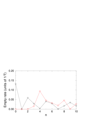
FIG. 1.: One–atom empty rates as a function of the trap level for the case of $eta=3.0$, and a laser pulse with detuning $\delta=s\omega$, with $s=8$ (diamonds) and $s=-3$ (circles).

FIG. 2.: Averaged population of the trap levels, for the case of $\eta=3.0$ and cooling cycles consisting of four pulses with durations $T=2\gamma/\Omega^{2}$, and detunings $\delta=s\omega$ with $s=-9,8,-10,-3$. The cases of (a) r=0.0, (b) r=0.4, (c) r=0.8, (d) r=1.2 and (e) r=5.0 are considered.

Fig. 2 shows the evolution of the averaged population of the level $n=1$ when $r$ grows. We have evolved the system under 5000 cooling cycles (to avoid the effects of the initial conditions), and performed the average from the cycle $5000$ until the cycle $15000$. In Fig. 2 we have depicted the averaged population distribution for the cases of (a) $r=0$ (ideal gas), (b) $r=0.4$, (c) $r=0.8$, (d) $r=1.2$, and (e) $r=5.0$. For the ideal–gas case $r=0$ one obtains that the population is completely condensed into the level $n=1$ [16]. When $r$ is increased the laser–induced condensation into the excited state $n=1$ is destroyed, but in a non–trivial way. We observe in Fig. 2 (b) that for $r=0.4$ the population is basically distributed in two well defined peaks, one in $n=1$ and the other in $n=7$. The reason for this behavior can be understood very well using Fig. 1. In absence of collisions the level $n=1$ is not emptied at all, while, as pointed out previously, $n=7$ is emptied, but slowly, and therefore at the end the population is finally transferred to the level $n=1$. However in the presence of collisions, level $n=1$ is still a dark–state for the laser, but it is emptied by the collisions with a frequency proportional to $N_{1}^{2}$. This means that the population is pumped into $n=1$ due to the laser cooling, but the more the population we pump into $n=1$ the more the level is emptied via collisions. This effect can be well illustrated by Fig. 3, where one can observe periods of filling of $n=1$ followed by abrupt decays of the level population. The emptying of level $n=1$ is mainly produced via collisions between two atoms in the level $n=1$ to produce two atoms in $n=0$ and $n=2$ respectively. The laser cooling provides a mechanism to repump such expelled population from the level $n=0$ and $n=2$ back to the level $n=1$. Such control is already maintained for large occupations of $n=1$, but in an unstable way, due to the highly non–linear character of the dynamics. A slight excess of population into the level $n=0$ and $n=2$ provoques a speed–up of the emptying process of $n=1$. This situation is reflected, for example, in the behavior of the system between cycles $4500$ and $5500$ in Fig. 3. In particular, level $n=1$ can become more emptied than $n=7$, and the latter turns to be the effective darkest level, i.e. the level less emptied. Therefore the population tends to be transferred into $n=7$. But, when $N_{7}$ increases so does the empty rate of the level $n=7$, which can become larger than that of $n=1$, and so on. Therefore, as consequence of this process a non–linear pseudo–oscillatory motion between the populations of $n=1$ and $n=7$ is produced, as observed in Fig. 3. This oscillatory motion leads to the two–peaked distribution of Figs. 2. Finally, when $r$ becomes very large the collision dynamics is much faster than the cooling time, and the peaked structure dissapears, as observed in Figs. 2 (c), (d) and (e). Observe that nevertheless the effects of the laser cooling mechanism are nevertheless present in Fig. 2 (f). In absence of laser cooling, it can be demonstrated that for $r=5$, the population has a maximum in $n=0$. On the contrary, in the presence of the laser, the population of $n=0$ is very efficiently and rapidly emptied by the pulse with detuning $s=8$, which is the most rapid cooling process. For larger $r$ even this process is eventually overcome, and one recovers the same distribution as that obtained only considering the collisions without laser cooling.

IV Three-dimensional results

In this section we analyze the case of the laser–cooling into the ground state of an isotropic three–dimensional harmonic trap, of frequency $\omega$. The numerical calculation of the system dynamics for the three–dimensional case is quite complicated, due to both the degeneracy of the levels, and the difficulties to obtain reliable values for the integrals $U(n_{1},n_{2},n_{3},n_{4})$. Therefore, we shall limit ourselves to the use of the ergodic approximation, i.e. we shall assume that states with the same energy are equally populated. The populations of the degenerate energy levels equalize on a time scale much faster than the collisions between levels of different energies, and than the laser–cooling typical time. This approximation leads to the correct steady–state distribution, although the dynamics can be slightly different than in the non–ergodic calculation [20].

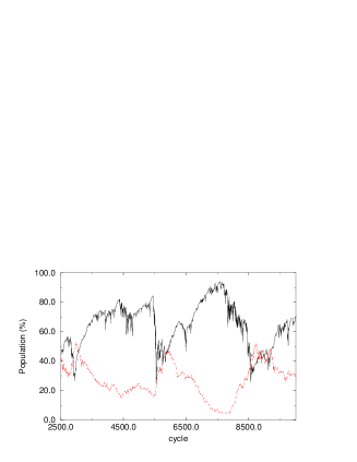
FIG. 3.: Detail of the dynamics of the populations of levels $n=1$ (solid line) and $n=7$ (dashed line), for the case of $\eta=3.0$, $r=0.4$. Each cooling cycle consists of four pulses with durations $T=2\gamma/\Omega^{2}$, and detunings $\delta=s\omega$ with $s=-9,8,-10,-3$. The non–linear pseudo–oscillation between $n=1$ and $n=7$ can be clearly observed.

Following ref. [29] the probability of a collision of two atoms in energy shells $n_{1}$ and $n_{2}$, to give two atoms in shells $n_{3}$ and $n_{4}$ (where this collision is assumed to change the energy distribution function), is of the form:

$$P(n_{1},n_{2}\rightarrow n_{3},n_{4})=\Delta(n_{j}+1)(n_{j}+2)$$ (41)

$$\times\frac{N_{n1}(N_{n2}-\delta_{n_{2},n_{1}})(N_{n_{3}}+g_{n_{3}})(N_{n_{4}}+g_{n_{4}}+\delta_{n_{3},n_{4}})}{g_{n_{1}}g_{n_{2}}g_{n_{3}}g_{n_{4}}},$$ (42)

where $g_{n_{k}}=(n_{k}+1)(n_{k}+2)/2$ is the degeneracy of the energy shell $n_{k}$, $n_{j}=min\{n_{1},n_{2},n_{3},n_{4}\}$, and $\Delta=(4a^{2}\omega^{2}m)/(\pi\hbar)\sim 1.5\times 10^{-5}$. Concerning the laser–cooling probabilities we shall use the same expressions as those already developed in Refs. [16].

In the following we simulate the evolution of the system by using again Monte Carlo simulations. Due to numerical limitations we consider a Lamb–Dicke parameter $\eta=2$. We assume as previously $\gamma=0.04\omega$ and $\Omega=0.03\omega$, and a number of atoms $N=133$. As a first step, we begin with a thermal distribution of mean $\langle n\rangle=6$, and evolve the system just with collisions, until obtaining a Bose–Eintein distribution (BED) (which does not coincide exactly with the thermodynamical one, due to finite–size effects), see Fig. 4. The distribution obtained in this initial step serves as the initial state for laser cooling. As we see, it already contains quite subtantial amount of atoms condensed in the ground state, but also a lot of uncondensed ones. Laser cooling will transfer the latter ones into the ground state. We apply our laser cooling cycles, each one of them composed by two laser pulses of detuning $\delta=s\omega$, with $s_{1,2}=-4,0$, and time duration $T=(2\gamma)/\Omega^{2}$. The laser pulses are emitted in three orthogonal directions $x$, $y$ and $z$, and are characterized by their respective rabi frequencies $\Omega_{x}=\Omega_{y}=\Omega$, $\Omega_{z}=A_{z}\Omega$. For the first pulse we assume $A_{z}=1$, while for the second one $A_{z}=-2$ is considered. With this choice, the second pulse is an ”interference”–dark–state pulse for the ground–state of the trap. Fig. 5(a) shows (dashed line) that these two pulses are able to condense the population into the ground state of the trap, in absence of collisions; in particular no confinement pulses (of detunings $\delta=-12\omega$ in this case) are needed. This is due to the bosonic enhancement and the fact that initially the system is already partially condensed. The dark–state pulse is neccesary to repump the population in those states of the energy shells $1$, $2$ and $3$, which are dark respect to the pulses with detuning $\delta=-4\omega$. Fig. 5 shows (solid line) the dynamics of the population of the ground-state in presence of collisions. After 600 cycles, all the population is transferred to the ground state of the trap. This means that applying the laser cooling scheme brigs the system into an effective BED of $T=0$. It is easy to undertand why the effect is maintained in presence of collisions, even considering that the collisional dynamics is much faster than the laser–cooling one. The laser–cooling mechanism tends to decrease the energy per particle (i.e. the chemical potential of the system), in the same way as evaporative cooling does, but without the losses of particles in the trap during the process. Thermalization via collisions brings the system to a lower temperature. Repeating the laser cooling sufficient times the system ends with an effective zero temperature. Finally, let us point out that some auxiliary pulses which are needed in the ideal gas, are not in presence of collisions. In particular for the previous example, the pulse of zero detuning (required for the ideal gas case, Fig. 5(b) dashed line) is no more needed, as shown in Fig. 5(b) (solid line). Thus, the laser–cooling scheme is not only possible in presence of collisions, but can be even significanly simplified.

FIG. 4.: Average of the population of the different energy shells, after evolving the system under collisions, starting from a themal distribution of $\langle n\rangle=6$.

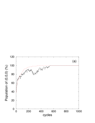
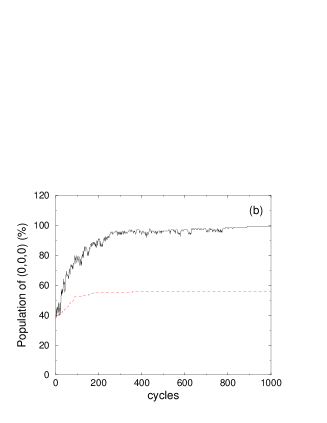
FIG. 5.: Dynamics of the population of the ground state of the trap for the case of $\eta=2$, $\gamma=0.04\omega$, $\Omega=0.03\omega$, $N=133$, starting from the BED distribution of Fig. 4. (a) Cooling cycles composed of two laser pulses of detunings $\delta=s\omega$, with $s_{1,2}=-4,0$, and $A_{z}=1,-2$ repectively, are used. The simulations taking into account the collisions (solid line) and no taking them into account (dashed line) are compared. (b) Same case, but only employing pulse $1$.

V Conclusions

In this paper, we have analysed the effects of the atom–atom collisions on the colective laser cooling of bosonic gases trapped in an harmonic trap, under the Festina–Lente condition. In particular, we have studied the case in which the mean–field energy provided by the atom–atom collisions is much smaller than the typical energy of the harmonic trap. Under such conditions, we have derived the ME which describes the system, and observed that such ME splits into two parts:(i) a purely collisional part which has the form of a QBME, and (ii) a purely laser–cooling part, which has the same form as the ME which describes the laser–cooling in absence of collisions. By using this ME, we have simulated the dynamics of the trapped gas for different situations. First, we have analysed the cooling into an excited state of a one–dimensional trap. We have observed that the transition from the ideal–gas limit (in which the atoms are completely condensed into the chosen excited state) to the case in which the collisions dominate the dynamics, is not trivial, specially when the collisional and cooling time scale are comparable. In such a case, cooling and collisional processes enter in competition, and new phenomena can appear, as for example unstable population of an excited state followed by abrupt population decays, and non–linear pseudo–oscillations between different trap levels. We have finally analyzed the laser–cooling into the ground state of an isotropic three–dimensional harmonic trap, by using the ergodic approximation. We have shown that, although the collisional time is typically much faster than the cooling time scale, the laser cooling allows to transform a BED with a finite temperature into an effective BED with zero temperature. The laser cooling reduces the chemical potential of the trapped atoms, while the collisions provide the thermalization.

Let us finally present important remarks concerning the scaling of our theory, the situation beyond the weak–condensation regime, and the problem of the two- and three–body losses in the trap. First, we stress that we have presented here the results obtained for $\eta=2,3$ only for the reasons of numerical complexity which grows rapidly with $\eta$. Qualitatively, the same results can be obtained for larger $\eta$’s, and therefore, for lower densities. In fact, we have observed similar results for $\eta=5$ in one dimensional simulations. If we increase $\eta$ by factor $F$, the corresponding density (for fixed $N$) decreases as $F^{-3}$, the three body loss rates as $F^{-6}$, whereas the trap frequency decreases as $F^{-2}$, which means that the corresponding cooling time (to fulfill the Festina Lente conditions) will increase as $F^{2}$, i.e. much less than the lifetime due to three-body collisions.

Beyond the weak condensation regime, the mean–field energy cannot be neglected, and therefore the trap levels are no more the harmonic ones. This has a two–fold consequence: (i) The levels of the trap are non–harmonic, i.e. they are not equally separated, because their energies become dependent on the occupation numbers; (ii) the wavefunctions are different, and in particular the condensate wavefunction becomes broader (we consider here only the case of repulsive interactions, $a>0$). The fact that the energy levels are not harmonic any more, complicates the laser cooling, but the use of pulses with a variable frequency and band–width should produce the same results as those presented here. The point (ii) implies that the central density of the interacting gas is much lower than the one predicted for noninteracting particles. In fact, the ratio between the interacting–gas central density (in Thomas–Fermi (TF) approximation) and the ideal–gas central density, goes as [30]

$$\frac{n_{TF}}{n_{ideal}}=\frac{15^{2/5}\pi^{1/2}}{8}\left(\frac{Na}{a_{HO}}\right)^{-3/5},$$ (43)

where the central density for the ideal case is given by $n_{ideal}=N/(\pi^{3/2}a_{HO}^{3})$.

The above result has important consequences, when one considers the problem of three–body collisions, which usually begin to play a role at densities of the order of $10^{15}$ atoms/cm³. For example, let us analyse the case of Sodium, for which $a_{R}=\sqrt{\hbar/m\omega_{R}}=0.132\mu{\rm m}$, and $a=2.75$nm. From the definition of $\eta$, $a_{HO}=\eta a_{R}$. For the ideal gas case, the regime in which three–body losses are important is reached for $N\simeq 12.8\eta^{3}$. For $\eta=8$ this means $N=6.5\times 10^{3}$. Amazingly, for the interacting gas, the same is true for $N\simeq 5.1\eta^{6}$, and therefore for $\eta=8$, the regime in which three–body losses are important is reached for $N=1.3\times 10^{6}$. Below this number, the interaction between the particles is dominated by the ellastic two–body collisions considered in this paper. As point out above, our laser cooling scheme could be extended beyond the weak–condensation regime, and therefore laser–induced condensations of more than $10^{6}$ atoms are feasible.

Concerning other loss mechanisms, we have to mention here the hyperfine changing two-body collisions, or generally speaking any inelastic two-body processes. These can be supressed completely if we cool atoms into the absolute ground internal state, which is possible in the dipole traps. For alkalis this is typically done by cooling to the lowest energy state in the lower hyperfine manifold (external static magnetic fields are used to split the levels within the hyperfine manifold).

Finally, yet another loss mechanism disregarded here is due to photoassociation, i.e. excitation of molecular resonances. This kind of loss rates are typically of the order $\gamma n(\lambda/2\pi)^{3}$ (where $\gamma$ is the linewidth of the auxiliary level $|r\rangle$, $\lambda$ is the laser wavelength, and $n$ is the atomic density), i.e. allow for achieving about $1000$ cooling cycles of duration $\simeq 1/\gamma$ provided the density remains smaller than $10^{12}-10^{13}$ atoms/cm². However, the photoassociation losses can be reduced by several orders of magnitude if the laser is red detuned, and tuned exactly in the middle of the molecular resonances [31] (note that this is the detuning respect to the one–photon transitions from the ground states to the state $|r\rangle$, and not the two–photon detuning). Other, possibility, is of course to use a more intense laser tuned below the Condon point, i.e. the minimum of the molecular potential.

We acknowledge support from Deutsche Forschungsgemeinschaft (SFB 407) and the EU through the TMR network ERBXTCT96-0002. We thank J. I. Cirac, Y. Castin, G. Birkl, K. Sengstock, W. Ertmer, T. Pfau and T. Esslinger for fruithful discussions.

REFERENCES

- [1] S. Chu, Nobel Lecture, Rev. Mod. Phys. 70, 685 (1998), C. Cohen–Tannoudji, Nobel Lecture, ibid., 707; W. D. Phillips, Nobel Lecture, ibid., 721.
- [2] M. H. Anderson J. R. Ensher, M. R. Matthews, C. E. Wieman and E. A. Cornell, Science 269, 198 (1995); K.B. Davis, M. O. Mewes, M. R. Andrews, N. J. van Drutten, D. S. Durfee, D. M. Kurn and W. Ketterle, Phys. Rev. Lett. 75, 3969 (1995); C. C. Bradley, C. A. Sackett and R. G. Hulet , ibid. 78, 985 (1997).
- [3] C. J. Myatt, E. A. Burt, R. W. Ghrist, E. A. Cornell and C. E. Wieman, Phys. Rev. Lett. 78, 586 (1997).
- [4] S. N. Bose, Z. Phys. 26, 178 (1924); A. Einstein, Sitzber. Kgl. Preuss. Akad. Wiss., p.261 (1924).
- [5] R. J. C. Spreeuw, T. Pfau, U. Janicke and M. Wilkens, Europhys. Lett. 32, 469 (1995).
- [6] U. Janicke and M. Wilkens, Europhys. Lett. 35, 561 (1996).
- [7] U. Janicke and M. Wilkens, Adv. At. Mol. Opt. Phys. 41, 261 (1999).
- [8] J. I. Cirac and M. Lewenstein, Phys. Rev. A 53, 2466 (1996).
- [9] A. Aspect, E. Arimondo, R. Kaiser, N. Vanteenkiste and C. Cohen-Tannoudji, Phys. Rev. Lett. 61, 826 (1988).
- [10] M. Kasevich and S. Chu, Phys. Rev. Lett. 69, 1741 (1992).
- [11] E. Arimondo and G. Orriols, Lett. Nuovo Cimento 17, 333 (1976).
- [12] D. W. Sesko, T. G. Walker and C. E. Wieman, J. Opt. Soc. Am B 8, 946 (1991); M. Olshan’ii, Y. Castin and J. Dalibard, Proc. 12th Int. Conf. on Laser Spectroscopy, M. Inguscio, M. Allegrini and A. Lasso, Eds. (World Scientific, Singapour, 1996); A. M. Smith and K. Burnett, J. Opt. Soc. Am. B 9, 1256 (1992); K. Ellinger, J. Cooper and P. Zoller, Phys. Rev. A 49, 3909 (1994).
- [13] Y. Castin, J. I. Cirac and M. Lewenstein, Phys. Rev. Lett. 80, 5305 (1998).
- [14] J. I. Cirac, M. Lewenstein and P. Zoller, Europhys. Lett. 35, 647 (1996).
- [15] L. Santos and M. Lewenstein, Phys. Rev. A (in press); see also G. Morigi, J. I. Cirac, M. Lewenstein and P. Zoller, Europhys. Lett 39, 13 (1997).
- [16] L. Santos and M. Lewenstein, Europhys. J. D, in press (1999); L. Santos and M. Lewenstein, Phys. Rev. A, in press (1999).
- [17] J. Stenger, S. Inouye, M. R. Andrews, H. J. Miesner, D. M. Stamper–Kurn and W. Ketterle, Phys. Rev. Lett. 82, 2422 (1999).
- [18] P. O. Fedichev, Yu. Kagan, G. V. Shlyapnikov and J. T. M. Walraven, Phys. Rev. Lett. 77, 2913 (1996).
- [19] C. W. Gardiner and P. Zoller, Phys. Rev. A, 55, 2902 (1997).
- [20] D. Jaksch, C. W. Gardiner and P. Zoller, Phys. Rev. A, 56, 575 (1997).
- [21] C. W. Gardiner and P. Zoller, Phys. Rev. A, 58, 536 (1998).
- [22] D. Jaksch,C. W. Gardiner, K. M. Gheri and P. Zoller, Phys. Rev. A, 58, 1450 (1998).
- [23] C. W. Gardiner and P. Zoller, cond-mat/9905087.
- [24] I. Marzoli, J. I. Cirac, R. Blatt and P. Zoller, Phys. Rev. A 49, 2771 (1994).
- [25] C. Gardiner, Handbook of Stochastical Methods, Springer Verlag,1985.
- [26] C. W. Gardiner, Quantum Noise (Springer-Verlag, Berlin, 1991).
- [27] H. Carmichael, An Open Systems Approach to Quantum Optics, Springer-Verlag, 1993.
- [28] H. Carmichael, Statistical Methods in Quantum Optics 1, Springer-Verlag, 1999.
- [29] M. Holland, J. Williams and J. Cooper, Phys. Rev. A 55, 3670 (1997).
- [30] F. Dalfovo, S. Giorgini, L. P. Pitaevskii, and S. Stringari, Rev. Mod. Phys. 77, 463 (1999).
- [31] T. W. Hijmans, G. V. Shlyapnikov and A. L. Burin, Phys. Rev. A 54 4332 (1996); K. Burnett, P. S. Julienne, and K.-A. Suominen, Phys. Rev. Lett. 77, 1416 (1996).