Natural Capacity of a System of Two Two-Level Atoms
as a Quantum Information Channel

Abstract

A system of two closely spaced atoms interacting through a vacuum electromagnetic field is considered. It is demonstrated that radiative decay in such a system resulting from photon exchange gives rise to a definite amount of information related to interatomic communication. Joint distributions of detection probabilities of atomic quanta and the corresponding amount of communication information are calculated.

I Introduction

Analysis of physical systems as potential sources of quantum information is becoming an urgent issue in the context of extensive research into the physical implementation of quantum computation techniques [1-3]. Such an analysis is inevitably associated with mathematical problems that differ from those encountered in the analysis of such systems as objects of conventional methods of physical experiments. One of the natural goals of the approach specified above is to reveal the possibilities of using specific physical mechanisms that would ensure information exchange between microscopic quantum systems employed as components of quantum data converters. In this respect, two-level atoms (TLAs) interacting through a vacuum electro-magnetic field can be considered as one of the fundamental systems of this type. Obviously, two two-level atoms (TTLAs) form an elementary system. Certain efforts have been already concentrated on the investigation of such a system [4-7]. The main problem encountered in the exact calculation of TTLA dynamics stems from the necessity to rigorously take into account relaxation processes simultaneously with reversible interactions.

In this paper, we investigate the process of radiative decay in a TTLA system in its pure form in the absence of an external field. We consider TTLA dynamics on a time scale $\tau\gg\tau_{r}$, i.e., for time intervals greater than the radiative decay time $\tau_{r}$ for a single atom. From the viewpoint of information transmission in a TTLA system, it is of interest to understand how much information is produced and stored in a system upon the completion of radiative decay processes in TLAs constituting the system under study and which type of information we deal with in this case. Evidently, such a formulation of the problem has no meaning for atoms separated by a distance on the order of or greater than the wavelength, i.e., for atoms in traps, which can be considered as one of the prototypes of a physical quantum processor [3]. In this case, all the dynamic variables of a TTLA system decay on the same time scale $\tau_{r}$. However, for atoms of the relevant variables continue to relax within much greater time intervals $\tau\gg\tau_{r}.$ Then, the information that relates the initial state of a TTLA system to its final state is stored. Such a geometry of a TTLA system may be implemented not only for atoms in dense media, but is also typical of impurity atoms adsorbed on a substrate. According to the experimental data of [8], impurity atoms under these conditions may preserve the discrete structure of atomic states and may be considered as microscopic quantum systems for quantum data con-version in a quantum computer. The mechanism behind the information exchange described above is associated with a relaxation photon exchange between closely spaced TLAs initially prepared in independent states. If the exchange rate $\gamma_{\rm ex}$ is close to the radiative decay rate $\gamma$ of TLAs, then a single-quantum diatomic state $\psi_{\rm a}=\mathop{\left|1\right\rangle}\nolimits\otimes\mathop{\left|0\right\rangle}\nolimits-\mathop{\left|0\right\rangle}\nolimits\otimes\mathop{\left|1\right\rangle}\nolimits$, which decays with a rate equal to $\gamma-\gamma_{\rm ex}$, exists within a time interval $\tau\gg\tau_{r}=\gamma^{-1}$. It is this singlet (in terms of a system of two spins) state that plays an important role in systems implementing the methods of quantum cryptography [9, 10]. The mechanism under consideration naturally governs quantum data exchange between TLAs.

In this paper, we restrict our consideration to a system of two closely spaced TLAs with a geometry of dipole moments shown in Fig. 1. Obviously, as long as the application of such a system is not specified, its information efficiency remains uncertain. Nevertheless, it seems appropriate to define the information efficiency in terms of the natural definition of the amount of data, which will be specified in this paper with the use of a given procedure of quantum measurement, without discussing the generalization of the considered approach. We assume that the information criterion employed in our study is sufficient for comparing different mechanisms of information exchange in terms of the information efficiency of feasible schemes for quantum computations using atomic transitions. In this paper, the definition of the amount of information will employ the Shannon definition of communication information corresponding to the probability distribution of measured energy quanta for each atom, which is described by a standard expression presented in [11].

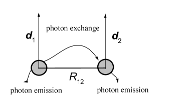
FIG. 1.: Geometry of a TTLA system and relaxation processes of natural radiative decay.

II Radiative decay in a system of two closely spaced atoms

The system under consideration (Fig. 1) consists of two TLAs undergoing spontaneous radiative decay of excited states through the interaction with an electro-magnetic vacuum, which is described in a standard manner as a thermal reservoir. The relaxation superoperator ${\cal L}_{\rm r}$ of radiative decay can be calculated for a system of closely spaced atoms in the same way as in the case of a single atom [12], i.e., with a standard formula of second-order perturbation theory in the Hamiltonian of the interaction of an atom with positive- and negative- frequency components $\hat{\xi}^{\pm}_{k\tau}=-{\bf d}^{k}_{12}\hat{\bf E}^{\pm}_{0}({\bf R}_{k},\tau)$ of (${\bf R}_{k}$ are the coordinates of atoms) produced by emission and absorption of photons of the vacuum electromagnetic field $\hat{\bf E}_{0}$. Representing superoperators with the use of a substitution symbol $\odot$ of an operator being transformed, we arrive at the following expression for the superoperator ${\cal L}_{\rm r}$ for several atoms in the Heisenberg representation (by analogy with the case of a single atom [13])

$${\cal L}_{\rm r} = -\lim\limits_{\Delta\to 0}\frac{1}{\hbar^{2}\Delta}\int\limits_{0}^{\Delta}\int\limits_{0}^{\tau_{2}}d\tau_{1}d\tau_{2}\mathop{\left\langle\left[\sum\limits_{k}\left(\hat{\sigma}^{+}_{k}\hat{\xi}^{-}_{k\tau_{1}}+\hat{\sigma}^{-}_{k}\hat{\xi}^{+}_{k\tau_{1}}\right),\left[\sum\limits_{m}\left(\hat{\sigma}^{+}_{m}\hat{\xi}^{-}_{m\tau_{2}}+\hat{\sigma}^{-}_{m}\hat{\xi}^{+}_{m\tau_{2}}\right),\odot\right]\right]\right\rangle}\nolimits_{\xi}$$ (1)

$$= \sum{\cal L}_{{\rm r}k}+\sum_{k\neq m}{\cal L}_{{\rm r}km}.$$ (2)

Here, ${\cal L}_{{\rm r}k}$ is the relaxation eigensuperoperator for an isolated $k$th atom due to spontaneous decay and ${\cal L}_{{\rm r}km}$ describe relaxation photon exchange between the $k$th and $m$th atoms,

$${\cal L}_{{\rm r}km}=-\frac{\gamma_{km}}{2}\left(\hat{\sigma}^{-}_{k}\hat{\sigma}^{+}_{m}\odot+\odot\hat{\sigma}^{-}_{k}\hat{\sigma}^{+}_{m}-\hat{\sigma}^{-}_{k}\odot\hat{\sigma}^{+}_{m}-\hat{\sigma}^{-}_{m}\odot\hat{\sigma}^{+}_{k}\right).$$ (3)

Here $\hat{\sigma}^{+}_{k}=\hat{P}^{k}_{12},$ $\hat{\sigma}^{-}_{k}=\hat{P}^{k}_{21}$, and $\gamma_{kl}$ is the relevant transition rate,

$$\gamma_{kl}=\frac{\omega_{\rm a}^{3}}{2\pi\hbar c^{3}}\int{\bf d}_{\bot}^{k}\cdot{\bf d}_{\bot}^{m}\exp\left(-i\omega_{\rm a}{\bf n}{\bf R}_{km}/c\right)d^{2}{\bf n},$$ (4)

where $\bf n$ is the vector along the direction of the emitted photon, ${\bf d}_{\bot}^{k}$ is the transverse component of the dipole moment, $\omega_{\rm a}$ is the frequency of atomic transitions, and ${\bf R}_{km}$ are the vectors of interatomic distances. In the case of two TLAs, along with the natural rate of radiative decay $\gamma$ for each atom, for the angle $\theta$ between parallel dipole moments ${\bf d}^{1,2}_{12}$ and ${\bf R}_{12}$ equal to $\pi/2$, we obtain a new relaxation constant of photon exchange $\gamma_{12}=\gamma_{\rm ex}$:

$$\gamma_{\rm ex}=g\gamma,\quad g=\frac{3}{2}\frac{\varphi\cos\varphi-\sin\varphi+\varphi^{2}\sin\varphi}{\varphi^{3}},$$ (5)

where the modulus of the parameter $g$ is less than unity, $\varphi=\omega_{\rm a}R_{12}/c$ is the phase delay of a signal between the atoms. For $\theta=\pi/2$ and $R_{12}\to 0$, we find that $g\approx 1-\varphi^{2}/5\to 1$, whereas in the case of anti-parallel dipole moments ${\bf d}^{1,2}_{12}$, we have $g\to-1$. Obviously, these two cases are equivalent to each other from the information point of view.

With the above-specified assumptions, the noise Liouvillian ${\cal L}_{\rm r}$ is invariant with respect to the permutation of atoms and, correspondingly, has no matrix elements that would couple symmetric and antisymmetric operators of an atomic system. Therefore, the representation basis is chosen in such a manner that $\hat{e}_{k}=\left(\hat{s}^{1}_{k}\otimes\hat{s}^{2}_{k}\right)/\sqrt{2},\;k=1,...,4;\quad\hat{e}_{k+4}=\left(\hat{s}^{1}_{i(k)}\otimes\hat{s}^{2}_{j(k)}+\hat{s}^{1}_{i(k)}\otimes\hat{s}^{2}_{j(k)}\right)/\sqrt{2},\;k=1,...,6$, and $\hat{e}_{k+10}=\left(\hat{s}^{1}_{i(k)}\otimes\hat{s}^{2}_{j(k)}-\hat{s}^{1}_{i(k)}\otimes\hat{s}^{2}_{j(k)}\right)/\sqrt{2},\;k=1,...,6,$ where a pair of indices $i(k)$ and $j(k)$ describes all possible combinations of pairs of single-atom basis vectors $\hat{s}^{1}_{i}$ and $\hat{s}^{2}_{j}$: $\{i(k)j(k)\}=(12,13,14,23,24,34)$. The vectors $\hat{s}^{1}_{i}$ and $\hat{s}^{2}_{j}$ are chosen as a basis of single-atom operators $\hat{I}/\sqrt{2}$, $(\hat{P}_{22}-\hat{P}_{11})/\sqrt{2}$, $(\hat{P}_{12}+\hat{P}_{21})/\sqrt{2}$, and $i(\hat{P}_{12}-\hat{P}_{21})/\sqrt{2}$, orthonormalized with respect to a scalar product $(\hat{A},\hat{B})={\rm Tr}\,\hat{A}^{+}\hat{B}$. Thus, the first ten basis elements describe symmetric atomic variables, whereas the last six basis elements describe antisymmetric atomic variables. Since, in the considered geometry, a laser field generates only symmetric excitations, the calculation of laser excitation is reduced to a ten-dimensional problem. However, this paper does not consider a procedure of the preparation of the initial state. We are interested only in the transformation of the initial state of the form $\hat{\rho}_{i}=\hat{\rho}^{(1)}\otimes\hat{\rho}^{(2)}$ in the process of relaxation.

Applying superoperator (1) to the basis elements $\hat{e}_{k}$, we obtain the following matrix representation for the relaxation operator:

$$L_{\rm r}=\left(\begin{array}[]{cc}L_{\rm SS}&\hat{0}\\ \hat{0}&L_{\rm AA}\end{array}\right)\,,$$ (6)

where $\hat{0}$ stands for a matrix with zero elements that complements the remaining submatrices up to a 16$\times$16 matrix, and

$$L_{\rm SS}=\left(\begin{array}[]{cc}L_{\rm SS}^{1}&0\\ 0&L_{\rm SS}^{2}\end{array}\right),$$

$$L_{\rm SS}^{1}=\gamma\left(\begin{array}[]{ccccc}0&0&0&0&-\sqrt{2}\\ 0&-2&g&g&0\\ 0&g&-1&0&-\displaystyle\frac{g}{\sqrt{2}}\\ 0&g&0&-1&-\displaystyle\frac{g}{\sqrt{2}}\\ 0&-\sqrt{2}&\displaystyle\frac{g}{\sqrt{2}}&\displaystyle\frac{g}{\sqrt{2}}&-1\end{array}\right),\quad L_{\rm SS}^{2}=\gamma\left(\begin{array}[]{ccccc}-\displaystyle\frac{1}{2}&0&-1-\displaystyle\frac{g}{2}&0&0\\ 0&-\displaystyle\frac{1}{2}&0&-1-\displaystyle\frac{g}{2}&0\\ \displaystyle\frac{g}{2}&0&-\displaystyle\frac{3}{2}-g&0&0\\ 0&\displaystyle\frac{g}{2}&0&-\displaystyle\frac{3}{2}-g&0\\ 0&0&0&0&-1\end{array}\right)$$

and

$$L_{\rm AA}=\gamma\left(\begin{array}[]{cccccc}-1&0&0&0&0&0\\ 0&-\displaystyle\frac{1}{2}&0&-1+\displaystyle\frac{g}{2}&0&0\\ 0&0&-\displaystyle\frac{1}{2}&0&-1+\displaystyle\frac{g}{2}&0\\ 0&-\displaystyle\frac{g}{2}&0&-\displaystyle\frac{3}{2}+g&0&0\\ 0&0&-\displaystyle\frac{g}{2}&0&-\displaystyle\frac{3}{2}+g&0\\ 0&0&0&0&0&-1\end{array}\right)$$

describe relaxation matrices for symmetric (S) and antisymmetric (A) variables. Expression (5) shows that these variables decay independently of each other, and small eigenvalues $\lambda_{k}\ll\gamma$ may exist only for the $L_{\rm SS}$ matrix.

III Determination of the amount of quantum information

The final state at the moment of time $t$ is described by a density matrix

$$\hat{\rho}_{f}={\cal S}^{+}(\hat{\rho}_{i}^{(1)}\otimes\hat{\rho}_{i}^{(2)})\,,$$ (7)

where $\cal S^{+}$ is the superoperator Hermitian-conjugate of the superoperator ${\cal S}=\exp\left({\cal L}_{\rm r}t\right)$, which describes the transformation of operators of physical variables in the Heisenberg representation. Here, we take into account two pairs of groups of dynamic variables—variables $\hat{A}_{1}$ and $\hat{A}_{2}$ related to atoms in the initial state at the moment of time $t=0$ before the interaction and the same variables at a certain final moment of time $t=\tau$ after the interaction, which determines transform $\cal S$. From the viewpoint of data exchange, it is of special interest to consider correlations between atomic variables at different moments of time, 0 and $\tau$, rather than correlations between variables $\hat{A}_{1}(\tau)$ and $\hat{A}_{2}(\tau)$ at the same moment of time, which are described by expression (7). We can calculate the information both between atomic TLA variables $\hat{A}_{1}(0)$ and $\hat{A}_{2}(\tau)$ and between TLA pairs $\hat{A}_{1}(0)\,,\hat{A}_{2}(0)$ and $\hat{A}_{1}(\tau)\,,\hat{A}_{2}(\tau)$.

To define the corresponding amount of information, we introduce the most typical class of measurement procedures that require the calculation of the relevant probability distributions. Consider a standard procedure of measurements with a coincidence scheme, which is described by a superoperator of the form ${\cal D}^{+}=\hat{\pi}_{n}^{+}\cdot\cdot\cdot\hat{\pi}^{+}_{1}\odot\hat{\pi}^{-}_{1}\cdot\cdot\cdot\hat{\pi}^{-}_{n}$, where $\hat{\pi}^{\pm}_{k}$ are some Hermitian-field conjugate pairs of operators, in particular, operators of creation and annihilation. Suppose that a set of operators $\hat{\pi}^{\pm}_{m}(k)$, $k=1,\ldots,n$ is defined for each $m$ such that the condition of completeness $\sum_{k}\hat{\pi}^{-}_{m}(k)\hat{\pi}^{+}_{m}(k)=\hat{I}$ is satisfied. In fact, it is of interest to consider sets of eigenprojectors corresponding to transitions between $n$ eigenstates $\psi_{k},\;\hat{A}_{m}\psi_{k}=\lambda_{k}\psi_{k}$, in accordance with relations $\hat{\pi}^{+}_{m}(k)=\mathop{\left|\psi_{k+1}\right\rangle}\nolimits\mathop{\left\langle\psi_{k}\right|}\nolimits$, where $n+1\to 1$ is taken for the brevity of notation. Here, we choose $\hat{A}_{m}=\hat{n}_{m}$ for a single atom, where $\hat{n}_{m}$ describes an operator of the number of an energy state at different moments of time $\tau_{m}$. For TLAs, we have $\hat{\pi}^{+}_{1}=\mathop{\left|2\right\rangle}\nolimits\mathop{\left\langle 1\right|}\nolimits,\;\hat{\pi}^{+}_{2}=\mathop{\left|1\right\rangle}\nolimits\mathop{\left\langle 2\right|}\nolimits,\;\hat{\pi}^{-}_{1}=\hat{\pi}^{+}_{2}$, and $\hat{\pi}^{-}_{2}=\hat{\pi}^{+}_{1}$. Now, we can introduce the relevant joint probability distribution,

$$P(k_{1},...,k_{n})=\mathop{\left\langle{\cal D}^{+}(k_{1},...,k_{n})\hat{\rho}\right\rangle}\nolimits,$$ (8)

where the superoperator ${\cal D}^{+}(k_{1},...,k_{n})=\hat{\pi}^{+}_{n}(k_{n})\cdot\cdot\cdot\hat{\pi}^{+}_{1}(k_{1})\odot\hat{\pi}^{-}_{1}(k_{1})\cdot\cdot\cdot\hat{\pi}^{-}_{n}(k_{n})$ introduces the corresponding measurement procedure, and averaging is performed over both TTLA and reservoir variables with allowance for the temporal evolution of the system under study within time intervals $\tau_{m+1}-\tau_{m}$ between the moments of time $\tau_{m}$ corresponding to the observation of detectable described by the set $\hat{\pi}^{\pm}_{m}$. A formula

$$\hat{\cal E}(k_{1},...,k_{n})={\cal D}(k_{1},...,k_{n})\hat{I}$$

relates the superoperator ${\cal D}^{+}(k_{1},...,k_{n})$ to a positive probability operator measure (POM) [1], which is conventionally employed in the quantum theory of information, i.e., a nonorthogonal expansion of unity $\hat{\cal E}(d\lambda),\;\int\hat{\cal E}(d\lambda)=\hat{I}$, which was introduced earlier in the theory of optimal quantum solutions (measurements) for the description of the procedure of a quantum measurement [14].

Here, we will use a set $\hat{\pi}^{\pm}_{1}$ that corresponds to the populations of atomic levels at the moment of time $\tau_{1}=0$ and an analogous set $\hat{\pi}^{\pm}_{2}$ corresponding to the moment of time $\tau_{2}$ such that the inequalities

$$\gamma\tau_{2}\gg 1\gg(1-g)\gamma\tau_{2}\,,$$ (9)

are satisfied. In other words, we assume that the distance between the atoms is sufficiently small, so that the condition $1-g\ll 1$ is met. Then, if inequalities (9) are satisfied for a transient superoperator ${\cal S}=\exp({\cal L}_{\rm r}\tau_{2})$ we can employ the following approximation:

$${\cal S}=\lim\limits_{\tau_{2}\to\infty}\exp({\cal L}_{\rm r}\mid_{g=1}\tau_{2})\,.{\hbox{}}$$ (10)

Under these conditions, the relaxation process brings a TTLA system into a stationary state, where the decay rate is equal to the rate of photon exchange, $g\gamma=\gamma$. In accordance with (8), this approximation is applicable on a time scale not greater than

$$\tau=[(1-g)\gamma]^{-1}\approx\frac{4\pi^{2}}{5}\left(\frac{R_{12}}{\lambda}\right)^{2}\gamma^{-1}\,,$$

where $\lambda$ is the radiation wavelength for transitions in TLAs.

Thus, we derive the following averaging rule for an operator of relaxation dynamics $\cal S$ with $n=2$ in terms of the Heisenberg representation in the case when quantum numbers $k_{1}$ of the first atom are measured at $t=0$ and analogous numbers $k_{2}$ of the second atom are measured at $t=\tau$:

$$P_{12}(k_{1},k_{2})={\rm Tr}\hat{\rho}\hat{\pi}^{-}_{1}(k_{1}){\cal S}\left[\hat{\pi}^{-}_{2}(k_{2})\hat{\pi}^{+}_{2}(k_{2})\right]\hat{\pi}^{+}_{1}(k_{1})\,.$$ (11)

With $n=4$, when the quantum numbers $k_{1}$ and $k_{2}$ of the first and second atoms are measured at the moment $t=0$ and the numbers $k_{3}$ and $k_{4}$ of the same atoms are measured at $t=\tau$, we have

$$P_{(12)(34)}(k_{1},k_{2},k_{3},k_{4})={\rm Tr}\hat{\rho}\hat{\pi}^{-}_{1}(k_{1})\hat{\pi}^{-}_{2}(k_{2}){\cal S}\left[\hat{\pi}^{-}_{1}(k_{3})\hat{\pi}^{-}_{2}(k_{4})\hat{\pi}^{+}_{2}(k_{4})\hat{\pi}^{+}_{1}(k_{3})\right]\hat{\pi}^{+}_{2}(k_{2})\hat{\pi}^{+}_{1}(k_{1})\,.$$ (12)

The amounts of information corresponding to these distributions are written as

$$I_{12}=H(P_{1})+H(P_{2})-H(P_{12})$$ (13)

in the case of separate atoms and

$$I_{(12)(34)}=H(P_{(12)})+H(P_{(34)})-H(P_{(12)(34)})$$ (14)

for pairs of atoms. Here, we employed a functional of the entropy $H(w)=-\sum\limits_{k}w(k)\log_{2}w(k)$ and single-moment probability distributions

$$P_{1}(k)=\sum\limits_{k_{2}}P_{12}(k,k_{2}),\quad P_{2}(k)=\sum\limits_{k_{1}}P_{12}(k_{1},k),$$

$$P_{(12)}(k_{1},k_{2})=\sum\limits_{k_{3},k_{4}}P_{(12)(34)}(k_{1},k_{2},k_{3},k_{4}),\quad P_{(34)}(k_{3},k_{4})=\sum\limits_{k_{1},k_{2}}P_{(12)(34)}(k_{1},k_{2},k_{3},k_{4}).$$

IV Results of calculations

In the absence of relaxation, i.e., with ${\cal S}=1$, the final state (7) coincides with the initial state,$\hat{\pi}^{\pm}_{2}=\hat{\pi}^{\pm}_{1}$, and joint distributions (11) and (12) can be represented as products of two independent distributions of the form $P_{1}(k_{1})P_{2}(k_{2})$ and $P_{1}(k_{1})P_{2}(k_{3})\delta(k_{1}-k_{2})\delta(k_{3}-k_{4})$, respectively, where $P_{l}(k)={\rm Tr}\,\hat{\pi}^{+}_{1}(k)\hat{\rho}_{i}^{(l})\hat{\pi}^{-}_{1}(k)$. Obviously, the corresponding amounts of information described by (13) and (14) are equal to zero in this case, i.e., the establishment of information occurs only in the process of relaxation.

Since we consider information in a quasi-stationary state, we have to calculate the transient superoperator (10) neglecting the decay of a single-quantum pure state $\psi_{\rm a}$, which occurs with a rate equal to $(1-g)\gamma$. To perform such a calculation, we use the following representation:

$${\cal S}=\lim\limits_{\lambda\to 0}\lambda\left({\cal L}_{\rm r}-\lambda I\right)^{-1},$$

where $I$ describes the identity superoperator represented by an identity matrix of the corresponding dimensionality, which is equal to 16 in the case of TTLAs. The resulting matrix representation ${\cal S}$ with $g=1$ is written as

$$S_{0}=\left(\begin{array}[]{cccccc}1&\displaystyle\frac{1}{2}&-\displaystyle\frac{1}{4}&-\displaystyle\frac{1}{4}&-\displaystyle\mathstrut\frac{3}{2\sqrt{2}}&\hat{0}\\ 0&\displaystyle\frac{1}{2}&\displaystyle\frac{1}{4}&\displaystyle\frac{1}{4}&-\displaystyle\mathstrut\frac{1}{2\sqrt{2}}&\hat{0}\\ 0&\displaystyle\frac{1}{2}&\displaystyle\frac{1}{4}&\displaystyle\frac{1}{4}&-\displaystyle\mathstrut\frac{1}{2\sqrt{2}}&\hat{0}\\ 0&\displaystyle\frac{1}{2}&\displaystyle\frac{1}{4}&\displaystyle\frac{1}{4}&-\displaystyle\mathstrut\frac{1}{2\sqrt{2}}&\hat{0}\\ &&&\hat{0}&&\hat{0}\end{array}\right).$$ (15)

For $g<1$, we derive an expression

$$S=\left(\begin{array}[]{cccccc}1&1&0&0&-\sqrt{2}&\hat{0}\\ &&&\hat{0}&&\hat{0}\end{array}\right),$$

which takes into account the decay of all the atomic states except for the ground one. The density matrix of the stationary state in this case is written as

$$\hat{\rho}^{(1+2)}(t)={\cal S}^{+}\hat{\rho}^{(1+2)}=\left(\begin{array}[]{cc}1&\hat{0}\\ \hat{0}&\hat{0}\end{array}\right).$$ (16)

Such a density matrix corresponds to a quantum-free state $\psi_{0}=\mathop{\left|0\right\rangle}\nolimits\otimes\mathop{\left|0\right\rangle}\nolimits$, i.e., the ground state of each atom, and, consequently, contains no information concerning the initial state of atoms. By contrast, the stationary density matrix corresponding to expression (14) is written as

$$\hat{\rho}^{(1+2)}(t)={\cal S}^{+}\hat{\rho}^{(1+2)}=\left(\begin{array}[]{cccc}1-A&0&0&0\\ 0&A/2&-A/2&0\\ 0&-A/2&A/2&0\\ 0&0&0&0\end{array}\right)\,,$$ (17)

where

$$A=\frac{1}{2}\left(\rho^{(2)}_{22}-\rho^{(2)}_{21}\rho^{(1)}_{12}-\rho^{(2)}_{12}\rho^{(1)}_{21}+\rho^{(1)}_{22}-2\rho^{(2)}_{22}\rho^{(1)}_{22}\right).$$

Such a density matrix corresponds to a mixed state of the form

$$\hat{\rho}^{(1+2)}(t)=(1-A)\psi_{0}\psi_{0}^{+}+A\psi_{\rm a}\psi_{\rm a}^{+},$$ (18)

In this case, the quantity $A$ represents the probability that a TTLA system resides in the singlet state $\psi_{\rm a}$ upon the completion of fast relaxation processes. In fact, off-diagonal elements of the density matrix with indices 12 and 21 are not involved in the matrix corresponding to the joint probability distribution of the quanta of the first and second atoms:

$$\parallel P(k_{1},k_{2})\parallel=\left(\begin{array}[]{cc}\rho^{(2)}_{22}\rho^{(1)}_{22}/4&(4-\rho^{(2)}_{22})\rho^{(1)}_{22}/4\\ \rho^{(2)}_{11}\rho^{(1)}_{11}/4&(3+\rho^{(2)}_{22})\rho^{(1)}_{11}/4\end{array}\right).$$ (19)

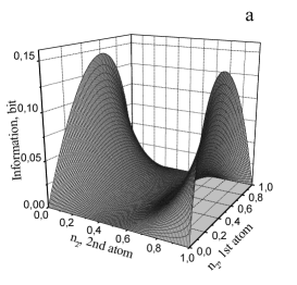
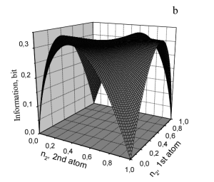
FIG. 2.: The amounts of information (a) between the initial state of the first atom and the final state of the second atom and (b) between the initial and final states of both atoms as functions of the mean populations of excited levels of the initial atomic states.

For $g=-1$, we obtain exactly the same distribution. The corresponding amount of information (13) is presented in Fig. 2a. The maximum of the information obtained between the final state of the second atom and the initial state of the first atom is achieved with a population $n_{2}=0$ or $n_{2}=1$ for the second atom and $n_{2}=-1+\sqrt{37}/4=0.521$ or, respectively, $n_{2}=2-\sqrt{37}/4=0.479$ for the first atom. The maximum amount of information is given by

$$\begin{array}[]{c}I_{12}^{\rm max}=\left(\displaystyle\frac{3}{2}-\displaystyle\frac{3\sqrt{37}}{16}\right)\log_{2}\left(\displaystyle\frac{3}{2}-\displaystyle\frac{3\sqrt{37}}{16}\right)-\left(2-\displaystyle\frac{\sqrt{37}}{4}\right)\log_{2}\left(2-\displaystyle\frac{\sqrt{37}}{4}\right)-\left(\displaystyle\frac{1}{2}+\frac{\sqrt{37}}{16}\right)\log_{2}\left(\displaystyle\frac{1}{2}+\frac{\sqrt{37}}{16}\right),\end{array}$$

and is approximately equal to 0.14 bit.

Joint two-atom two-moment distribution (12) is represented by a matrix

$$\parallel P(\{k_{1},k_{2}\},\{k_{3},k_{4}\})\parallel=\left(\begin{array}[]{cccc}0&0&0&\rho^{(2)}_{11}\rho^{(1)}_{22}/4\\ 0&\rho^{(2)}_{22}\rho^{(1)}_{22}&\rho^{(2)}_{11}\rho^{(1)}_{22}/4&\rho^{(2)}_{11}\rho^{(1)}_{22}/2\\ 0&\rho^{(2)}_{22}\rho^{(1)}_{11}/4&0&0\\ \rho^{(2)}_{22}\rho^{(1)}_{11}/4&\rho^{(2)}_{22}\rho^{(1)}_{11}/2&0&\rho^{(2)}_{11}\rho^{(1)}_{11}\end{array}\right).$$ (20)

The corresponding amount of information (14) in both atoms at the moment $t=\tau$ as compared with the initial state is presented in Fig. 2b. The maximum of this quantity is $I_{(12)(34)}^{\rm max}=0.322$ bit.

V Conclusions

The results of calculations presented above demonstrate that there exists a natural mechanism of information exchange between two closely spaced two-level atoms. If these atoms are initially prepared in statistically independent states, then, after a lapse of time $\tau$ such that $(1-g)\gamma\tau\ll 1\ll\gamma\tau$, where $\gamma$ is the decay rate of single-atom excitations and $g\approx 1$ is the efficiency of interatomic photon exchange with respect to single-atom decay, the procedure of counting the quanta of atomic excitations reveals the presence of nonzero information between the population of the second atom at the moment of time $\tau$ and the initial population of the first atom. The maximum amount of information $I_{\rm max}=0.14$ bit corresponds to the upper or lower initial state of the second atom and the mean population of the first atom close to 0.5. An analogous amount of information in both atoms is equal to $I_{\rm max}=0.322$ bit. Thus, a certain amount of information is produced without special efforts due to the specific features of spontaneous radiative decay in a system of closely spaced atoms.

Taking into account not only the relaxation but also resonant electrostatic dipole-dipole interaction, which is described by a Hamiltonian of the form $\hat{\cal H}_{C}=g_{C}(\hat{\sigma}_{1}^{+}\hat{\sigma}_{2}^{-}+\hat{\sigma}_{1}^{-}\hat{\sigma}_{2}^{+})$, one can easily verify by direct calculations that the superoperator of the transient distribution (15) remains unchanged. The same conclusion follows from the consideration of the symmetry of the system with allowance for the invariance of $\hat{\cal H}_{C}$ with respect to the permutation of atoms. Thus, electrostatic dipole-dipole interaction has no influence on relaxation data exchange as long as this interaction remains too weak to change the relaxation operator.

The results obtained above cannot be directly applied to the analysis of atoms on a surface because of large nonradiative dephasing rates, which gives rise to the main difficulty encountered when attempts are made to employ adsorbed atoms for the implementation of quantum computations [3]. However, we should note that, for closely spaced atoms, analysis of dephasing effects should take into account the specific features of relaxation processes associated with the interaction of atoms through dephasing excitations. The mechanism behind such an interaction should be, in a certain respect, similar to the mechanism considered in this paper.

- [1] 1997, Quantum Communication, Computing and Measurement, Hirota, O., Holevo, A. S., and Caves, C. M., Eds. (New York: Plenum).
- [2] Preskill, J., 1996, Panel discussion at the ITP Conf. on Quantum Coherence and Decoherence, December.
- [3] Cirac, J.I., Pellizzari, T., Polytos, J.F., and Zoller, P., 1997, Quantum Communication, Computing and Measurement, Hirota, O., Holevo, A.S., and Caves, C.M., Eds. (New York: Plenum), p. 159.
- [4] Gontier, Y., 1997, Phys. Rev. A 55, 2397.
- [5] Berman, P.R., 1997, Phys. Rev. A 55, 4466.
- [6] Power, E.A. and Thirunamachandran, T., 1997, Phys. Rev. A 56, 3395.
- [7] Murao, M., 1997, Quantum Communication, Computing and Measurement, Hirota, O., Holevo, A.S., and Caves, C.M., Eds. (New York: Plenum), p. 455.
- [8] Panov, V.I. et al., 1998, Appl. Phys. Lett. (in press).
- [9] Ekkert, A.K., 1991, Phys. Rev. Lett. 67, 661.
- [10] Bennet, C.H., 1991, Phys. Rev. Lett. 68, 557.
- [11] Klauder, J.R. and Sudarshan, E.C.G., 1968, Fundamentals of Quantum Optics (New York: Benjamin).
- [12] Lax, M., 1968, Fluctuations and Coherence Phenomena in Classical and Quantum Physics (New York: Gordon & Breach).
- [13] Grishanin, B.A., 1983, Zh. Eksp. Teor. Fiz. 85, 447.
- [14] Grishanin, B.A., 1973, Izv. Akad. Nauk SSSR, Ser. Tekh. Kiber. 11, no. 5, 127.