Hall Normalization Constants for the Bures Volumes of the $n$-State Quantum Systems

Abstract

We report the results of certain integrations of quantum-theoretic interest, relying, in this regard, upon recently developed parameterizations of Boya et al of the $n\times n$ density matrices, in terms of squared components of the unit $(n-1)$-sphere and the $n\times n$ unitary matrices. Firstly, we express the normalized volume elements of the Bures (minimal monotone) metric for $n=2$ and 3, obtaining thereby “Bures prior probability distributions” over the two- and three-state systems. Then, as a first step in extending these results to $n>3$, we determine that the “Hall normalization constant” ($C_{n}$) for the marginal Bures prior probablity distribution over the $(n-1)$-dimensional simplex of the $n$ eigenvalues of the $n\times n$ density matrices is, for $n=4$, equal to ${71680/\pi^{2}}$. Since we also find that $C_{3}=35/\pi$, it follows that $C_{4}$ is simply equal to $2^{11}C_{3}/\pi$. ($C_{2}$ itself is known to equal $2/\pi$.) The constant $C_{5}$ is also found. It too is associated with a remarkably simple decompositon, involving the product of the eight consecutive prime numbers from 3 to 23. We also preliminarily investigate several cases $n>5$, with the use of quasi-Monte Carlo integration. We hope that the various analyses reported will prove useful in deriving a general formula (which evidence suggests will involve the Bernoulli numbers) for the Hall normalization constant for arbitrary $n$. This would have diverse applications, including quantum inference and universal quantum coding.

Contents

toc

I INTRODUCTION

We make use of recently proposed parameterizations [1] (cf. [2]) — in terms of squared components of the unit $(n-1)$-sphere and the $n\times n$ unitary matrices — of the $n\times n$ density matrices. First (in sec. II), we derive (prior) probability distributions of particular interest over both the three-dimensional convex set of two-state quantum systems and the eight-dimensional convex set of three-state quantum systems. These distributions are the normalized volume elements of the corresponding Bures metrics on these systems. Hall [3] (cf. [4, 5, 6]) has contended that such distributions correspond to “minimal-knowledge” ensembles, that is the most random ensembles of possible states. In particular, for the two-dimensional quantum systems, he argues that the Bures metric provides such a minimal-knowledge ensemble, since it “corresponds to the surface of a unit four-ball, i. e., to the maximally symmetric space of positive curvature …This space is homogeneous and isotropic, and hence the Bures metric does not distinguish a preferred location or direction in the space of density operators” [3]. Somewhat contrarily though, Slater [7] has reported results (based on the concept of comparative noninformativities of priors, first expounded in [8]) that indicate the Bures metric generates ensembles that are less noninformative than other (monotone) metrics of interest.

The Bures metric fulfills the role of the minimal monotone metric [9, 10, 11], and has been the focus of a considerable number of studies [3, 7, 12, 13, 14, 15, 16]. “An infinitesimal statistical distance has to be monotone under stochastic mappings” [9, p. 786]. All stochastically monotone Riemannian metrics are characterized by means of operator monotone functions. Among all (suitably normalized) operator montone functions $f(t)$ with $f(1)=1$ and $f(t)=tf(t^{-1)}$, there is a minimal and a maximal one [18]. (The concept of a minimal metric was apparently introduced by Zolotarev in his extensive paper, “Metric distances in spaces of random variables and of their distributions” [17, sec. 1.4], but it is not entirely clear that the meaning there is the same as in the terminology “minimal monotone metric”.)

We should bear in mind, though — as emphasized by Petz and Sudár [9] — that, in strong contrast to the classical situation, in the quantum domain there is not a unique monotone metric, but rather a (nondenumerable) multiplicity of them. Their comparative properties need to be evaluated, before deciding which specific one to employ for a particular application. We repeat the concluding remarks of Petz and Sudár: “Therefore, more than one privileged metric shows up in quantum mechanics. The exact clarification of this point requires and is worth further studies.”

We have previously reported [19] (in terms of parameterizations other than that of Boya et al [1]) the Bures probability distribution for the two-state systems, and also [20] for an imbedding of these systems into a four-dimensional convex set of three-state systems, but the result below (11) for the full eight-dimensional convex set of three-state systems is clearly novel in nature. In fact, in [21, sec. II.E] we discussed certain (unsuccessful) efforts in these directions (although the volume element of the maximal monotone metric — which is not strictly normalizable — proved more amenable to analysis there).

In sec. III, we determine certain necessary elements for extending the work reported in sec. II to the higher-dimensional quantum systems ($n>3$). This involves finding the normalization constant ($C_{n}$), explicitly first discussed by Hall [3, eq. (25)], for the marginal Bures prior probability distribution over the $(n-1)$-dimensional simplex of the $n$ eigenvalues of the $n\times n$ density matrices. These constants are found to exhibit quite remarkable number-theoretic properties. It would, therefore, certainly be of substantial interest to find a general formula for $C_{n}$. Knowledge of the value of $C_{n}$, together with that of the invariant Haar element for $SU(n)$ — apparently presently available, however, in suitably parameterized form (cf. [22, 23]) for $n\leq 3$ [24, 25] — would allow one to construct the Bures prior probability distribution itself for the $n$-level quantum systems.

In an extensive study [26], Krattenthaler and Slater examined (in the framework of the two-state systems) the hypothesis that the normalized volume element of the Bures metric would function in the quantum domain in a role parallel to that fulfilled classically by the “Jeffreys’ prior” — that is, the normalized volume element of the unique monotone/Fisher information metric [27, 28]. In particular, they were interested in [26] in the possibility of extending certain (classical) seminal results of Clarke and Barron [29, 30]. They did conclude, however, contrary to their working hypothesis, that the normalized volume element of the Bures metric does not in fact strictly fullfill the same role as the Jeffreys’ prior (in yielding both the asymptotic minimax and maximin redundancies for universal coding/data compression), but it appears to come remarkably close to doing so (cf. Fig. 4). In sec. IV, for the cases $n=2$ and 3, the “quasi-Bures” prior probability distributions are presented that appear to fulfill this distinguished information-theoretic role.

II BURES PROBABILITY DISTRIBUTIONS OVER THE ${n\times n}$ DENSITY MATRICES

Boya et al [1] have recently “shown that the mixed state density matrices for $n$-state systems can be parameterized in terms of squared components of an $(n-1)$-sphere and unitary matrices”. The mixed state density matrix ($\rho$) is represented in the form,

$$\rho=UDU^{\dagger},$$ (1)

where $U$ denotes an $SU(n)$ matrix, $U^{\dagger}$ its conjugate transpose and $D$ a diagonal density operator, the diagonal entries ($d_{i}$’s) of which — being the eigenvalues of $\rho$ — are the squared components of the $(n-1)$-sphere. Thus, for $n=2$,

$$D=\pmatrix{\cos^{2}{\theta/2}&0\cr 0&\sin^{2}{\theta/2}\cr}\qquad 0\leq\theta\leq{\pi\over 2},$$ (2)

and, for $n=3$,

$$D=\pmatrix{\cos^{2}{\phi/2}\sin^{2}{\theta/2}&0&0\cr 0&\sin^{2}{\phi/2}\sin^{2}{\theta/2}&0\cr 0&0&\cos^{2}{\theta/2}\cr}\qquad 0\leq\theta,\phi\leq\pi.$$ (3)

(Note the differences in the ranges of angles used in the two cases. This will be commented upon in sec. III B.)

Biedenharn and Louck have presented [31, eq. (2.40)] the parameterization of an element of $SU(2)$,

$$U(\alpha\beta\gamma)=e^{-i\alpha\sigma_{3}/2}e^{-i\beta\sigma_{2}/2}e^{-i\gamma\sigma_{3}/2},$$ (4)

in terms of the Pauli matrices ($\sigma_{i}$’s) and three Euler angles — $0\leq\alpha<2\pi,0\leq\beta\leq\pi,0\leq\gamma<2\pi$ — with an associated invariant Haar measure [31, eq. (3.134)],

$$\mbox{d}\Omega_{2}={1\over 8}\mbox{d}\alpha\mbox{d}\gamma\sin{\beta}\mbox{d}\beta.$$ (5)

Byrd [24] (cf. [25]) has extended this approach to $SU(3)$. He obtains

$$U(\alpha,\beta,\gamma,\kappa,a,b,c,\zeta)=e^{i\lambda_{3}\alpha}e^{i\lambda_{2}\beta}e^{i\lambda_{3}\gamma}e^{i\lambda_{5}\kappa}e^{i\lambda_{3}a}e^{i\lambda_{2}b}e^{i\lambda_{3}c}e^{i\lambda_{8}\zeta},$$ (6)

where $\lambda_{i}$ denotes one of the eight $3\times 3$ Gell-Mann matrices [32]. The corresponding invariant element is

$$\mbox{d}\Omega_{3}=\sin{2\beta}\sin{2b}\sin{2\kappa}{\sin^{2}{\kappa}}\mbox{d}\alpha\mbox{d}\beta\mbox{d}\gamma\mbox{d}\kappa\mbox{d}a\mbox{d}b\mbox{d}c\mbox{d}\zeta,$$ (7)

with the eight Euler angles having the ranges,

$$0\leq\alpha,\gamma,a,c<\pi,\quad 0\leq\beta,b,\kappa\leq{\pi/2},\quad 0\leq\zeta<\sqrt{3}.$$ (8)

For our purposes, the Euler angle $\gamma$ for the case $n=2$ and $c$ and $\zeta$ in the case $n=3$ are irrelevant, as they “drop out” in the formation of the product (1). (I thank M. Byrd for this important observation.) So, we will employ below the appropriate conditional versions of these invariant measures (5) and (7) — the condition (a technical statistical term) corresponding, of course, to the ignoring of the indicated angles.

The Bures metric itself is expressible in the form [12, eq. (10)]

$$d_{B}^{2}(\rho,\rho+\mbox{d}\rho)=\sum_{i,j=1}^{n}{1\over 2}{{|<i|\mbox{d}\rho|j>}^{2}\over d_{i}+d_{j}},$$ (9)

where $|i>$ denotes the eigenvectors of the $n\times n$ density matrix $\rho$, $<j|$, the corresponding complex conjugate (dual) vectors, and the $d$’s are the associated eigenvalues. The parameterization of Boya et al is, then, particularly convenient, since the eigenvalues and eigenvectors of $\rho$ are immediately available. Our chief concern must, then, be to compute the complete Jacobian of the transformation to the set of parameters of Boya et al. (We shall note for further reference the occurrence of the term $d_{i}+d_{j}$ in (9). This, is of course, simply proportional to the arithmetic mean, $(d_{i}+d_{j})/2$. By replacing this term by (twice) the exponential/identric mean (23) of $d_{i}$ and $d_{j}$, that is $2I(d_{i},d_{j})$, we shall obtain the particular “quasi-Bures” distributions described in sec. IV.)

A The Bures case $n=2$

For the case $n=2$, the volume element of the Bures metric (9) is proportional to the product of the inverse of the square root of the determinant of $\rho$ (or, equivalently, the determinant of $D$) with two Jacobians. The first Jacobian (in line with the familiar practice in the theory of random matrices [33, eq. (3.3.5)]) is itself the product of $(d_{1}-d_{2})^{2}$ and the (conditional) invariant element (5). The second Jacobian, ${\sin{\theta}/2}$, corresponds simply to the transformation from cartesian coordinates to the squared polar coordinates employed in (2). Simplifying and normalizing the full product, we arrive at the probability density for the normalized volume element of the Bures metric over the three-dimensional convex set of two-state quantum systems. This density is

$$\mbox{d}p_{Bures:2}(\theta,\alpha,\beta)={\cos^{2}{\theta}\sin{\beta}\over{\pi^{2}}}\mbox{d}\theta\mbox{d}\alpha\mbox{d}\beta\qquad 0\leq\theta\leq{\pi\over 2},\quad 0\leq\alpha\leq 2\pi,\quad 0\leq\beta\leq\pi.$$ (10)

The expected values of the eigenvalues are, then, ${1/2\pm 4/3\pi}$.

B The Bures case $n=3$

For the case $n=3$, the volume element of the Bures metric is equal to the product of: (i) two Jacobians again, one of which now has the form $\big{(}(d_{1}-d_{2})(d_{1}-d_{3})(d_{2}-d_{3})\big{)}^{2}$ multiplied by the (conditional) invariant measure (7), while the other, $(\cos{{\theta\over 2}}\sin^{3}{{\theta\over 2}}\sin{\phi})/2$, corresponds to the transformation to squared spherical coordinates used in (3); and (ii) the reciprocal of the product of the square root of the determinant of $\rho$ (or, equivalently, of $D$) and the difference between the sum of the three principal minors of order two of $\rho$ (or, equivalently, of $D$) and the determinant itself. Since $|\rho|^{1/2}=(\cos{{\theta\over 2}}\sin^{2}{{\theta\over 2}}\sin{\phi})/2$, it can be seen that considerable cancellation occurs between the numerator and the denominator of the full product. The normalization of the resultant volume element required considerable manipulations using MATHEMATICA (basically involving reducing the problem to the simplest possible form at each stage of the integration process). We obtained the following Bures prior probability density over the eight-dimensional convex set of three-state (spin-1) quantum systems,

$$\mbox{d}p_{Bures:3}(\theta,\phi,\alpha,\beta,\gamma,\kappa,a,b)={35u\over 128{\pi}^{4}(35+28\cos{\theta}+\cos{2\theta}-8\cos{2\phi}{\sin^{4}{{\theta\over 2}}})}\mbox{d}\theta\mbox{d}\phi\mbox{d}\widetilde{\Omega}_{3},$$ (11)

where

$$u={\sin^{3}{{\theta\over 2}}}\big{(}(35+60\cos{\theta}+33\cos{2\theta})\cos{\phi}-{8\cos{3\phi}}{{\sin^{4}{{\theta\over 2}}}})^{2}\big{)},$$ (12)

and the conditional invariant element (cf. (7)) is

$$\mbox{d}\widetilde{\Omega}_{3}=\sin{2\beta}\sin{2b}\sin{2\kappa}{\sin^{2}{\kappa}}\mbox{d}\alpha\mbox{d}\beta\mbox{d}\gamma\mbox{d}\kappa\mbox{d}a\mbox{d}b.$$ (13)

The eight variables have the previously indicated ranges ((3), (8)). In Fig. 1, we display the two-dimensional marginal probability distribution of (11) over the parameters $\theta$ and $\phi$ (which are invariant under unitary transformations of $\rho$).

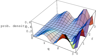
FIG. 1.: Bivariate marginal Bures prior probability distribution over the variables $\theta$ and $\phi$ for three-state systems

Let us note that the fully mixed state — corresponding to the $3\times 3$ diagonal density matrix with entries equal to $1/3$ — is obtained at $\phi=\pi/2,\theta=2\cos^{-1}({1/\sqrt{3})}\approx 1.91063$. The probability density (11) is zero at this distinguished point, as well as along the loci $\theta=0$ and $\phi=\pi/2$. (Wherever at least two of the eigenvalues of $\rho$ or, equivalently $D$, are equal, the density is zero.)

The one-dimensional marginal probability density (Fig. 2), obtained by integrating (11) over all variables except $\theta$, is

$$\mbox{d}\tilde{p}_{Bures:3}(\theta)={35\over 256}(-1533+2816\cos{{\theta\over 2}}-1988\cos{\theta}+1152\cos{{3\theta\over 2}}-447\cos{2\theta}+128\cos{{5\theta\over 2}})\sin^{3}{{\theta\over 2}}\mbox{d}\theta.$$ (14)

FIG. 2.: Univariate marginal Bures prior probability distribution over the variable $\theta$ for three-state systems

The relative maxima of this density are located at .914793, 2.2795 and $\pi$, while the relative minima are at 0, 1.59995 and 2.61732.

The one-dimensional marginal probability density (Fig. 3), obtained by integrating (11) over all variables except $\phi$, is

$$\mbox{d}\tilde{\tilde{p}}_{Bures:3}(\phi)={1\over 768\pi}\big{(}\cot{\phi}{\csc^{8}{\phi}}\big{(}110100480\tan^{-1}{[\cot{\phi\over 2}]}{\cos^{12}{{\phi\over 2}}}-26880(792(2\pi-\phi)\cos{\phi}+8\pi$$ (15)

$$(55\cos{3\phi}+3\cos{5\phi})+\phi(495\cos{2\phi}-220\cos{3\phi}+66\cos{4\phi}-12\cos{5\phi}+\cos{6\phi}))+16885656\sin{2\phi}$$

$$+5069937\sin{4\phi}+167012\sin{6\phi}-3(4139520\phi+124\sin{8\phi}-4\sin{10\phi}+\sin{12\phi})\big{)}\big{)}\mbox{d}\phi.$$

FIG. 3.: Univariate marginal Bures prior probability distribution over the variable $\phi$ for three-state systems

The limits of (15) as $\phi$ approaches 0 and $\pi$ are both equal to ${20\over 9\pi}\approx.707355$. (The density is highly oscillatory in the vicinity of these boundary points.) MATHEMATICA does, in fact, perform a symbolic/exact integration of (15), yielding the result 1. (Note that for our analyses below for $n>3$, we have found it necessary to rely upon numerical integrations, although the results obtained do appear to indicate that exact solutions exist, which in principle might be found with a powerful enough computer.) However, several warning messages are generated en route to this result, concerning indeterminate expressions and inconsistencies in the arguments of MeijerG functions (which are very general forms of hypergeometric functions) [34].

III HALL NORMALIZATION CONSTANTS FOR MARGINAL BURES PROBABILITY DISTRIBUTIONS OVER THE $(n-1)$-DIMENSIONAL SIMPLEX OF THE $n$ EIGENVALUES OF THE $n\times n$ DENSITY MATRICES

Let us note that Hall [3, eq. (24)] has, in fact, given an explicit formula for the volume element of the Bures metric on the $n\times n$ density matrices. This is (converting to the notation used above),

$$\mbox{d}V_{Bures:n}={\mbox{d}d_{1}\ldots\mbox{d}d_{n}\over(d_{1}\ldots d_{n})^{1/2}}\prod_{i<j}^{n}4{(d_{j}-d_{k})^{2}\over d_{i}+d_{j}}\mbox{d}x_{ij}\mbox{d}y_{ij},$$ (16)

where the real part of the $ij$-entry of the diagonalizing unitary matrix $U$ in formula (1) is represented by $x_{ij}$ and the imaginary part by $\pm iy_{ij}$. Since in the parameterization of Boya et al [1], which we have employed, one uses not these $x$’s and $y$’s, but rather the Euler angles parameterizing the unitary matrix $U$, we have been compelled to replace the differential elements $\mbox{d}x_{ij}\mbox{d}y_{ij}$ in (16) by the corresponding conditional form ($\mbox{d}\widetilde{\Omega}$) of the invariant (Haar) measures (5) and (7). One can, then, confirm that our presentation and results are fully consistent with the use of (16), bearing in mind the unit trace requirement that $d_{1}+\ldots+d_{n}=1$. Hall [3, eq. (25)] also expressed the marginal Bures probability distribution over the space of $n$ eigenvalues of $\rho$ as

$$\tilde{p}_{Bures:n}(d_{1},\ldots,d_{n})=C_{n}{\delta(d_{1}+\ldots+d_{n}-1)\over(d_{1}\ldots d_{n})^{1/2}}\prod_{i<j}^{n}{(d_{i}-d_{j})^{2}\over d_{i}+d_{j}}.$$ (17)

We shall report the values of the “Hall constants” $C_{n}$ for $n=2,3,4$ and 5, immediately below. (The results for $n>2$ are, apparently, new.)

A The Hall constants for $n=2$ and $n=3$

If, for consistency with our further results for $n>2$, we take $\theta\in[0,\pi]$ and not $[0,\pi/2]$ as in [1], then we find that $C_{2}$ equals $2/\pi\approx.63662$ (cf. [3, eq. (30)]). From the results of the analysis in sec. II B, we are able to determine, for the first time, apparently, that $C_{3}=35/\pi\approx 11.1408$. Let us note here that 35 is, of course, simply the product of proximate or neighboring prime numbers, that is, $35=5\cdot 7$.

B The Hall constant for $n=4$ and associated methodology

To continue the full line of research reported here for the cases $n=2,3$, to $n>3$, it would be useful to extend the work of Byrd and Sudarshan [24, 25] on the Euler angle parameterization of $SU(3)$ to such higher $n$. However, computation of the Hall constants $C_{n}$ (17) does not depend on parameterizations of $SU(n)$. We have, in fact, been able to obtain exceedingly strong numerical evidence that $C_{4}$ is, in fact, equal to ${71680/\pi^{2}}\approx 7262.7$. Let us, first, mention some methodological considerations useful in deriving this result (and, in general, $C_{n}$, $n>4$).

The parameterizations of Boya et al [1] of the diagonal $2\times 2$ and $3\times 3$ matrices differ, in that in the $2\times 2$ case (2) only matrices in which the (1,1)-entry is at least as great as the (2,2)-entry are generated (due to the restriction of the angular parameter, $\theta$, to the range $[0,\pi/2]$), while in the $3\times 3$ case (3), no order is imposed on the diagonal entries (the parameters $\theta$ and $\phi$ both varying freely between 0 and $\pi$). Now, in performing (the apparently necessary) numerical (as opposed to symbolic) integrations to obtain the Hall constants $C_{n}$ $(n>3)$, it seems to be considerably more computationally effective to integrate over only those diagonal matrices in which (say) the (1,1)-entry is no less than the (2,2)-entry, which in turn is no less than the (3,3)-entry, etc. (This helps to minimize troublesome oscillations.) Then, the result can be multiplied by the number ($n!$) of permutations of $n$ objects to yield $C_{n}$, since the result of the integration must be invariant under any other of the $n!-1$ possible orderings (permutations) that can be imposed on the diagonal entries of the $n\times n$ diagonal matrices. In precisely this manner, we were able to obtain (using the numerical integration of interpolating function command of MATHEMATICA) the result $71680.000001/\pi^{2}$ for $C_{4}$. This we take as overwhelming evidence that $C_{4}$, in fact, equals $71680/\pi^{2}$, particularly so, since 71,680 has the highly structured prime decomposition of $2^{11}\cdot 5\cdot 7$. (It is also interesting to note that $35=5\cdot 7$ appears in the numerator of $C_{3}$, that is, $35/\pi$, or, to the same effect, $C_{4}=2^{11}C_{3}/\pi$.

To illustrate the procedure followed, let us first parameterize the $4\times 4$ nonnegative diagonal matrices of trace unity in the following fashion (cf. (2), (3)),

$$D=\pmatrix{\cos^{2}{\theta/2}&0&0&0\cr 0&\sin^{2}{\theta/2}\cos^{2}{\phi/2}&0&0\cr 0&0&\sin^{2}{\theta/2}\sin^{2}{\phi/2}\cos^{2}{\zeta/2}&0\cr 0&0&0&\sin^{2}{\theta/2}\sin^{2}{\phi/2}\sin^{2}{\zeta/2}\cr}.$$ (18)

Then, the (truncated) region of integration employed above — corresponding to successively nonincreasing diagonal entries — can be described as $\zeta\in[0,\pi/2],\phi\in[0,f(\zeta)],\theta\in[0,f(\phi)]$, where $f(x)=2\cot^{-1}{(\cos{x/2})}$, rather than $\zeta,\phi,\theta\in[0,\pi]$, as in the apparently suggested parameterization of Boya et al [1], which would yield all possible diagonal matrices, without regard to the ordering of their elements.

If we construct a similar truncated region of integration in the case $n=3$, then we find that the expected values of the eigenvalues are .802393, .181878 and .0157299. In the $n=2$ case, the analogous values are (as previously noted), $1/2\pm 4/3\pi$, that is .924413, and .0755868.

C The Hall constant for $n=5$

We have also attempted to compute $C_{5}$, in the manner of sec. III B, with the use of MATHEMATICA. We obtained (using the Gauss-Kronrod integration method with a working precision of twenty-one digits, rather the machine precision of sixteen) the result $2342475135.00/\pi^{2}$. Now, it is most interesting to note (particularly, in light of our results for $C_{n}$, $n<5$, that

$$2,342,475,135=21\Pi_{i=2}^{9}P_{i}=21(3\cdot 5\cdot 7\cdot 11\cdot 13\cdot 17\cdot 19\cdot 23),$$ (19)

where $P_{i}$ denotes the $i$-th prime number (taking the sequence of primes to be $2,3,5,\ldots$). Thus, we have acquired strong evidence that, in fact, $C_{5}=2342475135/\pi^{2}$. (As a simple exercise, we looked at the one hundred thousand consecutive integers containing 2,342,475,135 as their midpoint, and computed all their prime decompositions. All the others had at least one prime factor greater than 23.) The seemingly independent factor of 21 in (19) will also apparently be found below in the (odd) case $n=7$.

1 Prime factorials

In [35], the product of the primes less than or equal to $p$ is denoted $p\#$. (The issue there, as in several of the works cited there, was to test $p\#\pm 1$ for primality (cf. [36]).) Let us point out a 1952 article [37], entitled “Tables of logarithms of the prime factorials from 2 to 10007” (a synopsis of which can be found in Mathematical Reviews 16, 112f). It is noted that by the prime number theorem [38] the ratio of the sum of the logarithms of the primes from 2 to $p$ to $p$ itself approaches 1 as $p\rightarrow\infty$. So, if it eventuates that the general formula for $C_{n}$, at least for odd $n$, contains a term of the form $p(n)\#$, where $p(n)$ is a prime as a function of $n$, which grows indefinitely large with $n$ itself, then it should be possible to asymptotically replace $p(n)\#$ by $e^{p(n)}$. (“A version of the prime number theorem states that the product of the primes less than $x$ is asymptotically $e^{x}$ [citing the well-known treatise [39, Theorem 434]], but the error term is notoriously large, so it is probably unrealistic to expect to be able to compute far enough to get within the necessary epsilon” [40].) We also observe that with the use of Wilson’s theorem [41], $(p-1)!\equiv-1\mbox{mod}{p}$, one could express $p\#$ in terms of the (more) standard factorial function $p!$. (In [42], the primes are defined in terms of factorials.)

Let us point out that Ellinas and Floratos have recently studied the “prime decomposition” of an $n\times n$ density matrix into a sum of separable density matrices with dimensions determined by the coprime factors of $n$ [43] (cf. [44]).

D Preliminary investigations of the Hall constant for $n>5$, with the use of quasi-Monte Carlo integration

1 $n=6$

Of course, as the dimensionality of the $n$-state quantum systems increases (that is, $n$ itself increases), the numerical integrations required to sufficiently narrow estimates of the corresponding Hall constant become increasingly more difficult, and it is hard to judge what is precisely the optimum numerical/programming strategy to employ. Following the methodology outlined in sec. III B, based on the ordering of the eigenvalues, MATHEMATICA did yield (using the standard default options) an estimate of $C_{6}$, representable in the form, $1.4616286\cdot 10^{16}/\pi^{3}$ (although diagnostics as to inadequate precision were issued during the course of the computation). This result, coupled with our observation of the pattern of $C_{n}$ for $n<6$, might lead us to speculate that the numerator of $C_{6}$ is either the seventeen-digit number, $14,616,907,579,654,144=2^{41}\cdot 17^{2}\cdot 23$ or $14,623,504,649,420,800=2^{42}\cdot 5^{2}\cdot 7\cdot 19$, with the denominators, in both cases, being $\pi^{3}$.

When we employed the quasi-Monte Carlo (Halton-Hammersley-Wozniakowski) procedure [45, chap. 3] [46] of MATHEMATICA, to numerically integrate over a hypercube of volume $\pi^{5}$ (corresponding, thus, now to no particular distinguished ordering of the six eigenvalues), we obtained (with no diagnostics at all being generated in two separate analyses — having set maxima of ten and fifty million sample points) a result of the form $1.536355674\cdot 10^{16}/\pi^{3}$. To a very high accuracy, this numerator can be approximated by $15,363,556,773,986,304=2^{28}\cdot 3^{4}\cdot 13^{2}\cdot 37\cdot 113$ for the numerator of the presumptive value of $C_{6}$ (with denominator, again, $\pi^{3}$). Sloan and Woźniakowski have noted that recently “Quasi-Monte Carlo algorithms have been successfully used for multivariate integration of high dimension $d$, and were significantly more efficient than Monte Carlo algorithms” [47]. However, in comparing the two sets of results here for $n=6$ it is very important to bear in mind that MATHEMATICA sets its precision and accuracy objectives much lower when Monte Carlo procedures are employed [46]. (Of course, these default values can be reset, but in the preliminary analyses reported here, they have not been, though we intend to do so in future studies.)

2 $n=7$

The quasi-Monte Carlo MATHEMATICA procedure produced an estimate (with no accompanying diagnostics, having set a maximum of four million sample points) of $C_{7}$ as $2.4811899\cdot 10^{24}/\pi^{3}$. The numerator of this fraction (cf. (19)) could be approximated (to a relative error of less than three-tenths of one percent) by the product of 21 and the (eighteen) consecutive primes from 2 to 61 (in the notation of [35], this is $61\#$), that is, $C_{7}=21\Pi_{i=1}^{18}P_{i}/\pi^{3}$. However, this degree of accuracy does not at all seem satisfactory, particularly in light of the proximate results for $n=6$ and 8, though odd $n$’s appear to present greater computational challenges.

3 $n=8$

The quasi-Monte Carlo procedure estimated $C_{8}$ as $4.1836777028\cdot 10^{35}/\pi^{4}$ (though, unlike the $n=6,7$ cases, a failure to converge was reported — that is, with the preassigned use of at most ten million sample points). Nonetheless, this outcome can be fit to a very high accuracy (less than one part in one hundred million) by taking $C_{8}$ to be $2^{89}\cdot 3^{2}\cdot 5\cdot 13^{2}\cdot 31\cdot 47\cdot 61/\pi^{4}$.

E $n\geq 9$

For the case $n=9$, convergence was not obtained with the use of six million sample points. The result given was $7.631832917\cdot 10^{47}/\pi^{4}$. We have also made tentative attempts, using the quasi-Monte Carlo procedure again, to estimate $C_{n}$ for $n=10$ and 11 (but it appears that considerable investment of computer resources is needed for sufficiently satisfactory answers). For $n=10$, based on a maximum of two million sample points, convergence was not obtained and the result $6.334733996\cdot 10^{62}/\pi^{5}$ reported. (No related decomposition was immediately apparent.) For $n=11$ and 12, using a maximum of one million sample points in both cases, the results $3.254198489\cdot 10^{78}/\pi^{5}$ and $5.218327334\cdot 10^{97}/\pi^{6}$ were gotten (without convergence or any obvious associated simple prime decompositions, however). Our impression is that the computations are considerably more difficult for the odd values of $n$ than for the even, which may be some reflection of the simpler formulas displayed above for even $n$ (cf. [48, 49]). (For $n>7$, the MATHEMATICA compiler was unable to handle the small numbers appearing in the calculation, and then proceeded with the use of the uncompiled evaluation, leading to slower running times [46].) Of course, there exists a wide range of possible approaches to numerical integration problems of this kind, including, certainly, the use of alternative programming languages, in particular, FORTRAN. The trade-offs between these various options need to be assessed.

As a reference point, against which one can attempt to compare the (reciprocals of the) several values of $C_{n}$ above, let us recall that the area of an $n$-sphere of radius $r$ is given by $2\pi^{n/2}r^{n-1}/\Gamma(n/2)$ [50]. Also of similar interest is Euler’s formula

$$\zeta(2n)={(-1)^{n-1}\over 2(2n)!}(2\pi)^{2n}B_{2n},\quad n=1,2,3,\ldots$$ (20)

where $\zeta(s)$ is the Riemann zeta function, $\sum_{n\geq 1}n^{-s}$, and $B_{n}$ is the (necessarily rational) $n$-th Bernoulli number [51, Vol. I, pp. 75 and 211]. (The values of $\zeta(n)$ for positive odd integers $n$, however, have not been expressed in such a simple form [52, Vol. III, p. 1695]. Infinite series representations are, in fact, reported in [48, 49].) Initial attempts to find an explanatory formula for the sequence of (integral) numerators of $C_{n}$, using on-line programs of C. Krattenthaler (“Rate”) [53, App. A] and of N. Sloane (“superseeker”) [54], did not succeed. However, we did eventually find a somewhat intriguing connection (further buttressed by some related analyses, discussed below in sec. III G) between the results here and sequence A035077 of [54], which gives the denominators of partial sums of $B_{2n}$. The numerator of: (1) $C_{2}$ is (rather trivially) twice the first entry in this sequence; (2) $C_{3}$ is one-half the fourth entry; (3) $C_{4}$ is $2^{10}=1024$ times the fourth entry; and (4) $C_{5}$ is 63 times the thirteenth entry of A035077. (We note that Donaldson has found simple proofs of various formulas for symplectic volumes involving Bernoulli numbers [55, 56, 57].)

F Average von Neumann entropy of $n$-state quantum systems with respect to Bures prior probability distributions

As one application of these computations of the Hall constants ($C_{n}$), let us note that with respect to the Bures probability distribution (10) the average von Neumann entropy, $-\mbox{Tr}\rho\log{\rho}$, is exactly $2\log{2}-7/6\approx.219628$ nats for the two-state systems and, now using numerical integration, .507937 nats for the three-state systems (cf. [58]). (Since we employ the natural logarithm here, the unit of information is the nat, which is equivalent to $1/\log{2}\approx 1.4427$ bits.) This latter result, to a high degree of precision — that is, to ten significant places, can, in fact, be written as $3\log{3}-3917/1405$. We also computed the Bures average entropy for the four-state quantum systems, obtaining .751771 nats. To eight significant places, this can be written as $4\log{4}-32135/6704$. Similarly, for $n=5$, using our knowledge of $C_{5}$, we obtain an average entropy of .954103 nats. This is closely approximated (to at least nine places, according to our calculations) by $5\log{5}-40045/5648$.

G Auxiliary analyses of variations of Hall integrals and the role of Bernouilli numbers

Since it appeared to be quite challenging to determine the Hall constants ($C_{n}$) for $n>5$, we thought that it might be revealing (possibly helpful in deriving a general formula for arbitrary $n$), as well as being of independent interest, to investigate more tractable variations. To do so, we replaced the exponent two in (16) and (17) by either one (corresponding to real quantum systems) or four (for quaternionic quantum systems) [33], and other positive integer values of less immediate physical interest, as well.

For the $n=3$ (spin-1) quaternionic case (that is, using an exponent of four), the counterpart of the previously derived (sec. III A) Hall constant $35/\pi$ is $1616615/{226\pi}=5\cdot 7\cdot 11\cdot 13\cdot 17\cdot 19/226\pi$. (The numerator here is one-half the tenth member of the sequence A035077, comprised of denominators of partial sums of the Bernoulli numbers $B_{2n}$ [54].) When we use an exponent of six, the result is $100280245065/88252\pi=3\cdot 5\cdot 7\cdot 11\cdot 13\cdot 17\cdot 19\cdot 23\cdot 29\cdot 31/88252\pi$. (This numerator is precisely the seventeenth member of A035077.)

If we use an exponent of one (corresponding to the case of real quantum systems), the result is $1/4\pi$, and if we employ an exponent of three, the normalization constant is $105/128\pi=3\cdot 5\cdot 7/128\pi$. (The numerator here is the fifth member of A035077.) For an exponent of five, we have $15015/8192\pi=3\cdot 5\cdot 7\cdot 11\cdot 13/8192\pi$, the numerator being three times the seventh entry of Sloane’s sequence. For an exponent of seven, the result was the eleventh member of the sequence A035077, that is, 969969, divided by $262144\pi$.

When an inquiry was made of Neil Sloane as to whether to his knowledge there were any published discussions of this sequence, he replied “No, I was just looking at various sequences of important rationals, and thought that the pair A035078/A035077 should be in the database”. (However, he later pointed out that the von Staudt-Clausen Theorem [59, p. 10] was relevant to questions involving sums of Bernoulli numbers.) For the case $n=3$, MATHEMATICA rejected our efforts to compute any further exact integrals having integer exponents greater than seven. (It would appear that the use of an exponent of eight would be associated with the octonionic quantum systems [60].)

For the analogous set of variations with $n=2$, use of odd exponents in (16) and (17) lead to divergent results. For an exponent of two, the result is $2\pi$, for four, $8/3\pi$, for six, $16/5\pi$, for eight, $128/35\pi$, ….

For comparable scenarios based on $n=4$, we were unable to proceed with exact integrations. Our numerical computation of the analog of the Hall constant employing an exponent of unity (the real quantum case), yielded $\pi^{2}/.079271$. But we were unable to determine if this result bore any relation to the sequence A035077.

IV QUASI-BURES PROBABILITY DISTRIBUTIONS OVER THE $n\times n$ DENSITY MATRICES

In line with the work reported in [26], it would be of interest to obtain formulas for the averages over the eight-dimensional convex set of $3\times 3$ density matrices ($\rho$) with respect to the Bures prior probability distribution (11) of the $m$-fold tensor products of $\rho$. As $m\rightarrow\infty$, the relative entropy of these products with respect to the averaged $3^{m}\times 3^{m}$ density matrix gives us the (Bures) asymptotic redundancy for the universal quantum coding of three-state systems.

A The quasi-Bures case $n=2$

In [26] and further yet unreported work, the Bures prior probability density (10) for the two-state systems was found to closely resemble the (what we term “quasi-Bures”) probability density,

$$\mbox{d}p_{quasi:2}(\theta,\alpha,\beta)=.226231(\tan^{\sec{\theta}}{\theta/2})\cos{\theta}\cot{\theta}\sin{\beta}\mbox{d}\theta\mbox{d}\alpha\mbox{d}\beta,\qquad 0\leq\theta\leq{\pi\over 2},\quad 0\leq\alpha\leq 2\pi,\quad 0\leq\beta\leq\pi$$ (21)

which yields, it appears, both the asymptotic minimax and maximin redundancies (as “Jeffreys’ prior” [27] does classically [29, 30]). This common value, if one ignores the error term, as appears to be legitimate, is $(3\log{m})/2-1.77062$, while the Bures probability distribution (10) has been shown to be, incorporating the error term, associated with an asymptotic redundancy of $(3\log{m})/2-1.77421+O(1/\sqrt{m})$ [26, p. 29]. In general, for any probability distribution $w(\theta),\theta\in[0,\pi/2]$, the asymptotic redundancy for the two-state quantum systems takes the form,

$${3\over 2}\log{{m\over 2\pi}}-{1\over 2}-2\log{\sin{\theta}}+2(\sec{\theta})\log{\tan{{\theta\over 2}}}-\log{w(\theta)}+o(1).$$ (22)

Standard variational arguments can, then, be used to show (ignoring the error term, the legitimacy of which seems plausible, but has not yet been rigorously justified) that the particular $w(\theta)$ yielding both the maximin and minimax redundancies is simply proportional to the $\theta$-dependent part of $p_{quasi:2}(\theta,\alpha,\beta)$, indicated in (21).

The reciprocal of the corresponding “Morozova-Chentsov function” $c(x,y)$ [9, 10] for (21) is the exponential or identric mean [61, eq. (1.3)] of $x$ and $y$,

$$I(x,y)=e^{-1}(x^{x}/y^{y})^{{1\over x-y}},\quad x\neq y$$ (23)

($I(x,x)=x$), while for the Bures (minimal monotone) metric, it is the (more commonly encountered) arithmetic mean $(x+y)/2$. The associated operator monotone functions [9, 10] are $f(t)=(1+t)/2$ for the Bures metric, and $f(t)=t^{t/(t-1)}/e$, for the metric giving (21). (The Morozova-Chentsov functions fulfill the relation $c(x,y)=1/yf(x/y)$.) Perhaps the exponential mean arises in this context because the von Neumann entropy is the logarithmic relative entropy, and of course the exponential and logarithmic functions are inverses of one another. This leads us to speculate that if one were to employ, following [11], the “quadratic relative entropy” or the “Bures relative entropy” instead, then, in the parallel universal coding context, the minimax/maximin would be achieved by the means corresponding to the new forms of inverse functions. While the logarithmic relative entropy is based on the operator convex function, $g(t)=-\log{t}$, the quadratic form relies upon $g(t)=(t-1)^{2}$ and the Bures form on $g(t)=(t-1)^{2}/(t+1)$ [11]. Here, $f(t)=(t-1)^{2}/(g(t)+tg(1/t))$.

In Fig. 4, we jointly display the univariate marginal probability distributions of (10) and (21), revealing that they closely resemble one another, with the quasi-Bures distribution assigning relatively greater probability to the states more pure in character ($\theta\leq.443978$).

FIG. 4.: One-dimensional marginals of the ($n=2$) Bures probability distribution (10) and the quasi-Bures distribution (21) (assuming greater values for $\theta\in[0,.443978]$), which yields both the asymptotic minimax and maximin redundancies for the universal quantum coding of two-state systems

B The quasi-Bures case $n=3$

The three-state counterpart of (21) (that is, the probability distribution associated with the exponential/identric mean, rather than the arithmetic mean, as for such Bures distributions) is

$$\mbox{d}p_{quasi:3}(\theta,\phi,\alpha,\beta,\gamma,\kappa,a,b)=.000063495u({\tan^{(1+\sec{\phi})}}{\phi/2}){\csc^{4}{{\theta\over 2}}}{\csc^{6}{{\phi\over 2}}}$$ (24)

$$(\cos{{\phi\over 2}}\tan{{\theta\over 2}})^{{16{\cos^{2}{{\phi\over 2}}}{\sin^{2}{{\theta\over 2}}}\over{v+w}}}(\sin{{\phi\over 2}}\tan{{\theta\over 2}})^{2-{8(1+\cos{\theta})\over{w-v}}}\mbox{d}\theta\mbox{d}\phi\mbox{d}\widetilde{\Omega}_{3},$$

where $u$ is given in (12), $\mbox{d}\widetilde{\Omega}_{3}$ in (13) and

$$v=2+6\cos{\theta},\quad w=\cos{(\theta-\phi)}-2\cos{\phi}+\cos{(\theta+\phi)}.$$ (25)

The corresponding two-dimensional marginal probability distribution over the variables $\theta$ and $\phi$ is exhibited in Fig. 5.

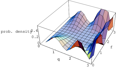
FIG. 5.: Bivariate marginal of the quasi-Bures probability distribution (24) over the variables $\theta$ and $\phi$, for three-state systems

As would be anticipated from Fig. 4, this figure closely resembles Fig. 1. In Fig. 6, we show the result obtained by subtracting the bivariate marginal Bures probability distribution shown in Fig. 1 from its quasi-Bures counterpart in Fig. 5.

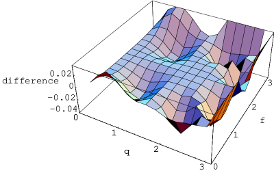
FIG. 6.: Difference obtained by subtracting the three-state Bures bivariate marginal probability density in Fig. 1 from the quasi-Bures one, associated with the exponential/identric mean, displayed in Fig. 5

C Quasi-Bures counterparts of Hall (Bures) normalization constants

If we replace the term $d_{j}+d_{k}$, occurring in the denominator of the expression (17), by (twice) the exponential/identric mean (23) of $d_{j}$ and $d_{k}$, that is, $I(d_{i},d_{j})$, the resultant expression becomes a formula for $\tilde{p}_{quasi:n}(d_{1},\ldots,d_{n})$, now interpreting $C_{n}$ to be the normalization constant for the corresponding quasi-Bures probability distribution. For $n=2$ then (taking $\theta\in[0,\pi]$ and not $[0,\pi/2]$ as in [1]), rather than $2/\pi\approx.63662$, we obtain .769427, and for $n=3$, instead of $35/\pi\approx.089759$, we find .138681.

V CONCLUDING REMARKS

We hypothesize that the (full eight-dimensional) quasi-Bures probability distribution (24) associated with Fig. 5 will furnish the common asymptotic (minimax and maximin) redundancies for universal quantum coding in that higher-dimensional setting, paralleling the result (not yet fully formally demonstrated, however) for the three-dimensional convex set of two-state systems (cf. [62]). In this regard, it might prove computationally convenient, as a heuristic device, to replace the quasi-Bures probablity distributions by their (closely approximating) Bures analogues, since certain exact (symbolic) integrations are achievable (at least, for the cases $n=2,3$) with the Bures distributions, but apparently not with the quasi-Bures ones, for which numerical methods seem to be necessary.

Although a parameterization of SU(4) is not relevant, as already noted, to the computation of the Hall constant $C_{4}$, that is, $71680/\pi^{2}$, and to that of the corresponding average (von Neumann) entropy (sec. III F), it would be essential in investigating the universal coding of four-state quantum systems, since the tensor products of $4\times 4$ density matrices have to be calculated and it would, therefore, be necessary to implement formula (1). In a personal communication, M. Byrd has indicated that he has undertaken the (challenging) task of developing such an (Euler angle) parameterization of $SU(4)$.

Such a parameterization of $SU(4)$ — in conjunction with the knowledge, acquired here, of $C_{4}$ — might also prove of value in estimating the volume of $2\times 2$ separable quantum states [2, 63] and lead to numerically more stable results than those reported in [64, Table I], since the “over-parameterizations” of the unitary matrices used there could then be avoided, due to the “dropping out” (as pointed out for $n=2,3$ immediately after (8) above) of certain Euler angles in the formation of the product (1). We also note that in [64] (cf. [65]), the Bures (minimal monotone) metric was found to yield higher a priori probabilities of entanglement than other monotone metrics (in particular, the Kubo-Mori-Bogoliubov and maximal ones). Presumably, even in any computationally improved form of analysis, this conclusion would be unaltered.

We have also pursued a traditional (pseudo-random number) Monte Carlo approach to estimating the Hall normalization constants for $2\leq n\leq 16$. However, the degrees of precision attained were not satisfactory. (For discussions of the comparative computational complexities of the pseudo- and quasi-Monte Carlo methods, see [47, 66].)

We are presently attempting to obtain a more precise estimate of the Hall constant $C_{6}$, in particular, using non-Monte Carlo (that is, adaptive) integration methods. Our best current estimate of $C_{6}$ is $1.534836628\cdot 10^{16}/\pi^{3}$. The numerator can be very well approximated by $15348366279966720=2^{33}\cdot 3\cdot 5\cdot 7^{2}\cdot 11\cdot 13\cdot 17$, which seems more satisfactory than the results reported in sec. III D 1, based on the quasi-Monte Carlo procedure. Now, it is most interesting to note that this numerator is precisely $2^{33}\cdot 7$ times the ninth entry of the sequence A035077, we have repeatedly referenced above. We are also compelled to observe that our educated conjecture as to the numerator of $C_{7}$ (sec. III D 2) is exactly forty-two times the thirty-third entry — which we had to compute ourselves, since Sloane’s published list does not extend this far — of A035077.

- [1] L. J. Boya, M. Byrd, M. Mims, and E. C. G. Sudarshan, Density Matrices and Geometric Phases for -State Systems, quant-ph/9810084.
- [2] K. Życzkowski, P. Horodecki, A. Sanpera, and M. Lewenstein, Phys. Rev. A 58, 883 (1998).
- [3] M. J. W. Hall, Phys. Lett. A 242, 123 (1998).
- [4] M. J. W. Hall, Phys. Rev. A 59, 2602 (1999).
- [5] P. Staszewski, Rep. Math. Phys. 13, 67 (1978).
- [6] M. A. Rieffel, Metrics on State Spaces, math.OA/9906151.
- [7] P. B. Slater, Phys. Lett. A 247, 1 (1998).
- [8] B. Clarke, J. Amer. Statist. Assoc. 91, 173 (1996).
- [9] D. Petz and C. Sudár, J. Math. Phys. 37, 2662 (1996).
- [10] D. Petz, Lin. Alg. Applics. 244, 81 (1996).
- [11] A. Lesniewski and M. B. Ruskai, Monotone Riemannian Metrics and Relative Entropy on Non-Commutative Probability Spaces, math-ph/9808016.
- [12] M. Hübner, Phys. Lett. A 163, 239 (1992).
- [13] M. Hübner, Phys. Lett. A 179, 226 (1993).
- [14] S. L. Braunstein and C. M. Caves, Phys. Rev. Lett. 72, 3439 (1994).
- [15] J. Dittmann, Sem. Sophus Lie 3, 73 (1993).
- [16] J. Dittmann, J. Phys. A, 32, 2663 (1999).
- [17] V. M. Zolotarev, Math. USSR Sbornik 30, 373 (1976).
- [18] F. Kubo and T. Ando, Math. Ann. 246, 205 (1980).
- [19] P. B. Slater, J. Math. Phys. 38, 2274 (1997); 37, 2682 (1996).
- [20] P. B. Slater, J. Phys. A 29, L271 (1996).
- [21] P. B. Slater, Volume Elements of Monotone Metrics on the Density Matrices as Densities-of-States for Thermodynamic Purposes. II, quant-ph/9802019.
- [22] K. Życzkowski and M. Kuś, J. Phys. A 27, 4235 (1994).
- [23] M. Poźniak, K. Życzkowski, and M. Kuś, J. Phys. A 31, 1059 (1998).
- [24] M. Byrd, J. Math. Phys. 39, 6125 (1998).
- [25] M. Byrd and E. C. G. Sudarshan, J. Phys. A 31, 9255 (1998).
- [26] C. Krattenthaler and P. B. Slater, Asymptotic Redundancies for Universal Quantum Coding, quant-ph/9612043 (to appear in IEEE Trans. Inform. Th.).
- [27] R. E. Kass, Statist. Sci. 4, 188 (1989).
- [28] L. C. Kwek, C. H. Oh, and X.-B. Wang, J. Phys. A 32, 6613 (1999).
- [29] B. S. Clarke and A. R. Barron, IEEE Trans. Info. Th. 36, 453 (1990).
- [30] B. S. Clarke and A. R. Barron, J. Statist. Plann. Inf. 41, 37 (1994).
- [31] L. C. Biedenharn and J. D. Louck, Angular Momentum in Quantum Physics, (Addison-Wesley, Reading, 1981).
- [32] I. Lukach and Ya. A. Smorodinskii, Sov. J. Nucl. Phys. 27, 888 (1978).
- [33] M. L. Mehta, Random Matrices (Academic, San Diego, 1991).
- [34] V. Kiryakov, J. Phys. A 30, 5085 (1997).
- [35] C. K. Caldwell, Math. Comp. 64, 889 (1995).
- [36] P. W. Shor, SIAM J. Comput. 26, 1484 (1997).
- [37] F. J. Duarte, Estados Unidos de Venezuela Bol. Acad. Ci. Fiz. Mat. Nat. 15, 3 (1952).
- [38] P. T. Bateman and H. G. Diamond, Amer. Math. Mon. 103, 729 (1996).
- [39] G. H. Hardy and E. M. Wright, An Introduction to the Theory of Numbers, (Clarendon, Oxford, 1960).
- [40] R. K. Guy and J. L. Selfridge, Amer. Math. Mon. 105, 766 (1998).
- [41] N. Robbins, Fibonacci Quart. 36, 317 (1998).
- [42] J. V. Matiajasevich, Zap. Nauch. Sem. Leningrad Otdel. Mat. Inst. Steklov (LOMI) 68, 62 (1977).
- [43] D. Ellinas and E. G. Floratos, J. Phys. A 32, L63 (1999).
- [44] J. M. Luck, P. Moussa, and M. Waldschmidt, Number Theory and Physics, (Springer-Verlag, Berlin, 1990).
- [45] M. Drmota and R. F. Tichy, Sequences, Discrepancies and Applications, (Springer-Verlag, Berlin, 1997).
- [46] S. Saarinen, MATHEMATICA in Educ. and Res. 5, 23 (1996).
- [47] I. H. Sloan and H. Woźniakowski, J. Complexity 14, 1 (1998).
- [48] M.-P. Chen and H. M. Srivastava, Results Math. 33, 179 (1998).
- [49] D. Cvijović and J. Klinowski, Proc. Amer. Math. Soc. 125, 1263 (1997).
- [50] B. A. Fusaro. Amer. Math. Mon. 80, 179 (1973).
- [51] A. Terras, Harmonic Analysis on Symmetric Spaces and Applications I and II, (Springer-Verlag, Berlin, 1985-88).
- [52] K. Ito, Encyclopedic Dictionary of Mathematics, (MIT Press, Cambridge, 1987).
- [53] C. Krattenthaler, Advanced determinant calculus, math.CO/9902004.
- [54] N. J. A. Sloane and S. Plouffe, Encyclopaedia of Integer Sequences, (Academic Press, San Diego, 1995).
- [55] S. K. Donaldson, Topological Methods in Modern Mathematics (Publish and Perish, Houston, 1993)
- [56] E. Witten, Commun. Math. Phys. 141, 153 (1991).
- [57] L. Jeffrey and J. Weitsman, Math. Ann. 307, 93 (1997).
- [58] D. N. Page, Phys. Rev. Lett. 71, 1291 (1993).
- [59] H. Rademacher, Topics in Analytic Number Theory, (Springer-Verlag, Berlin, 1973).
- [60] S. De Leo and K. Abdel-Khalek, Prog. Theor. Phys. 96, 823 (1996).
- [61] F. Qi, Proc. Roy. Soc. Lond. A, 454, 2723 (1998).
- [62] R. Jozsa, M. Horodecki, P. Horodecki, and R. Horodecki, Phys. Rev. Lett. 81, 1714 (1998).
- [63] K. Życzkowski, On the volume of the set of mixed entangled states II, quant-ph/9902050 (to appear in Phys. Rev. A).
- [64] P. B. Slater, J. Phys. A 32, 5261 (1999).
- [65] P. B. Slater, Essentially All Gaussian Two-Party Quantum States are a priori Nonclassical but Classically Correlated, quant-ph/9909062.
- [66] K. Frank and S. Heinrich, J. Complexity 12, 287 (1996).