Efficient implementation of selective recoupling in heteronuclear spin systems using Hadamard matrices

Abstract

We present an efficient scheme which couples any designated pair of spins in heteronuclear spin systems. The scheme is based on the existence of Hadamard matrices. For a system of $n$ spins with pairwise coupling, the scheme concatenates $cn$ intervals of system evolution and uses at most $cn^{2}$ pulses where $c\approx 1$. Our results demonstrate that, in many systems, selective recoupling is possible with linear overhead, contrary to common speculation that exponential effort is always required.

I Introduction

In recent proposals to perform quantum computation in nuclear spin systems using nuclear magnetic resonance (NMR) techniques [1, 2, 3, 4], coupled logic operations are performed using spin-spin couplings that occur naturally in molecular systems. While this is straightforward for small systems with a few spins, generalization to complex molecular structures has been challenging. The complication is caused by the many spin-spin couplings which occur along with the desired one. This fundamental task to turn off spurious evolution is so difficult that, coercing a complex system to do nothing [5] – ceasing all evolution – can be just as difficult as making it do something computationally useful.

The task of turning off all couplings is known in the art of NMR as decoupling; doing this for all but a select subset of couplings is known as selective recoupling. A common method to perform these tasks is to interrupt the free evolution by carefully chosen pulses. These pulses are single spin-1/2 (qubit) operations that transform the hamiltonian in the time between pulses in such a manner that unwanted evolutions in consecutive time intervals cancel out each other.

Pulse sequences which perform selective recoupling are generally difficult to find for a large system. Each pulse simultaneously affects many coupling terms in the hamiltonian. To turn off all but one of the coupling terms, these pulses have to satisfy many simultaneous requirements. Ingenious sequences have been found for usual NMR applications [6, 7, 8] but they do not address the problems relevant to quantum computation. In usual NMR applications, the structure of the spin systems is not known a-priori. Therefore, pulse sequences are designed to address all the spins together rather than individual spins. Quantum computation brings new requirements, and initial efforts [9] have been made to develop pulse sequences to satisfy these needs; however, to-date, schemes have necessitated resources (such as total number of pulses applied) exponential in the number of spins being controlled.

In this paper, we present an efficient scheme to perform selective recoupling. In contrast to the situation with traditional NMR, this scheme addresses the problem relevant to NMR quantum computation, in which the molecular structure is assumed to be well-known, and spins are individually addressible. The method is related to a class of well-known matrices called Hadamard matrices. We derive from any $n\times n$ Hadamard matrix a pulse scheme that decouples $n$ spins using $n$ time intervals and ${\cal O}(n^{2})$ pulses. This decoupling scheme can easily be modified (i) to remove Zeeman evolution and (ii) to implement selective recoupling. This completes the construction for $n$ spins whenever $n\times n$ Hadamard matrices exist. When $n\times n$ Hadamard matrices do not exist, a scheme for $n$ spins can still be constructed using larger existing Hadamard matrices. In doing so, an extra amount of effort is required, but this can be bounded using existence properties of Hadamard matrices. Altogether, the scheme requires $cn$ time intervals and less than $cn^{2}$ pulses, where $c\approx 1$ with upper bound $c\leq 2$. Our method applies whenever the spins couple pairwise and have very different Zeeman frequencies, such as in heteronuclear spin systems.

The paper is structured as follows. In Section II, we review relevant concepts in NMR quantum computing and re-state the problem precisely. In Section III, we first motivate the construction of the decoupling scheme with examples, and then describe the general construction related to Hadamard matrices. Important properties of Hadamard matrices are summarized. Modifications of the decoupling scheme to perform selective recoupling are described. We conclude with some general remarks and discussions of various properties and limitations of the scheme.

II NMR quantum computing and the statement of the problem

In this section, we describe the NMR system and describe how a universal set of (non-fault tolerant) operations [10, 11, 12], namely, the single qubit operations and the controlled-NOT gate, can be realized using basic NMR primitives.

We shall consider a physical system which consists of a solution of identical molecules. Each molecule has $n$ non-magnetically equivalent nuclear spins which serve as qubits. A static magnetic field is applied externally along the $+\hat{z}$ direction. This magnetic field splits the energy levels of the spin states aligned with and against it. This is described in the hamiltonian by the Zeeman terms, which, in the energy eigenbasis, are given by

$${\cal H}_{\rm Z}=-\frac{1}{2}\sum_{i}\hbar\omega_{i}\sigma_{z}^{(i)}\,,$$ (1)

where $i$ is the spin index, $\omega_{i}/2\pi$ is the Zeeman frequency for the $i$-th spin, and $\sigma_{z}^{(i)}$ is the Pauli matrix operating on the $i$-th spin. The convention $\hbar=1$ is used for the rest of the paper. The spins have very different Zeeman frequencies, a situation loosely termed as “heteronuclear” in this paper.

Nuclear spins can interact via the dipolar coupling [7, 13]. This is given by the hamiltonian

$${\cal H}_{\rm d}=\sum_{i<j}g_{ij}^{\rm d}\left[\rule{0.0pt}{10.33327pt}\vec{\sigma}^{(i)}\cdot\vec{\sigma}^{(j)}-3(\hat{r}_{ij}\cdot\vec{\sigma}^{(i)})\otimes(\hat{r}_{ij}\cdot\vec{\sigma}^{(j)})\right]\,,$$ (2)

where $\hat{r}_{ij}$ denotes the unit displacement vector from the $i$-th to the $j$-th spin, and $g_{ij}^{\rm d}$ denotes the coupling constant between them. Spin-spin coupling can also be mediated by coupling to electrons. This indirect coupling has a tensor part and a scalar part. The tensor part is usually of the same form as ${\cal H}_{\rm d}$. The scalar part is given by the hamiltonian

$${\cal H}_{\rm s}=\sum_{i<j}g_{ij}^{\rm s}\vec{\sigma}^{(i)}\cdot\vec{\sigma}^{(j)}\,.$$ (3)

If the molecules tumble fast and isotropically, dipolar coupling and indirect tensor coupling will be averaged away; otherwise, the physics can be more complicated. However, in the presence of a strong external magnetic field, only the secular part (terms that commute with ${\cal H}_{\rm Z}$) is important [7, 13]. For a heteronuclear system, the resulting coupling becomes

$${\cal H}_{\rm c}=\sum_{i<j}g_{ij}^{\rm c}\sigma_{z}^{(i)}\otimes\sigma_{z}^{(j)}\,,$$ (4)

independent of the original form of coupling.

Single qubit operations are performed by applying pulsed radio frequency (RF) magnetic fields along some directions $\hat{\eta}$ perpendicular to the static field. To address the $i$-th spin, the frequency of the RF field is chosen to approximate $\omega_{i}/2\pi$. When the $\omega_{i}$’s are very different, very short pulses can be used, so that during the pulses, all other evolutions are negligible except for the rotation operator $e^{-i\frac{\theta}{2}\vec{\sigma}^{(i)}\cdot\hat{\eta}}$ where $\theta$ is proportional to the pulse duration and the power. The Lie group of all single qubit operations can be generated by rotations about $\hat{x}$ and $\hat{y}$. Our scheme uses only rotations of $\theta=\pi$ along $\hat{x}$, which implement $\sigma_{x}$ (up to an irrelevant overall phase) on the spins being addressed. We denote this operation by $X$, superscripted by the spin index whenever appropriate.

Coupled operations such as controlled-phase-shift or controlled-NOT acting on the $i$-th and the $j$-th spins can be performed given the primitive,

$$Z\!\!Z_{ij}=e^{-i\frac{\pi}{4}\sigma_{z}^{(i)}\otimes\sigma_{z}^{(j)}}\,.$$ (5)

For instance, a controlled-NOT from the $i$-th to the $j$-th spin can be implemented by

$$e^{-i\frac{\pi}{4}\sigma_{y}^{(i)}}e^{i\frac{\pi}{4}\sigma_{x}^{(i)}}e^{i\frac{\pi}{4}\sigma_{y}^{(i)}}e^{-i\frac{\pi}{4}\sigma_{x}^{(j)}}e^{i\frac{\pi}{4}\sigma_{y}^{(j)}}Z\!\!Z_{ij}e^{-i\frac{\pi}{4}\sigma_{y}^{(j)}}\,.$$ (6)

The ultimate goal is to be able to efficiently realize arbitrary quantum operations on an $n$ spin system with arbitrary couplings. In this paper, we consider a more limited objective, which can now be stated precisely, using the definitions of Eq.(1), Eq.(4), and Eq.(5):

Given a heteronuclear system of $n$ spins with free evolution $e^{-i({\cal H}_{\rm Z}+{\cal H}_{\rm c})t}$, controlled using typical RF pulses, how can $Z\!\!Z_{ij}$ be implemented efficiently?

III Construction of the scheme

We will first construct a decoupling scheme to remove the entire coupling term ${\cal H}_{\rm c}$ in the total evolution. The scheme is derived from Hadamard matrices, which will be reviewed. Methods to remove ${\cal H}_{\rm Z}$ and to implement selective recoupling will be described afterwards.

A Construction of the decoupling scheme

To construct the decoupling scheme, we only consider ${\cal H}_{\rm c}$ in the evolution. Effects of ${\cal H}_{\rm Z}$ can be included later since all matrix exponents commute.

To motivate the general construction, we analyze the simplest example of decoupling two spins. The evolution operator for an arbitrary duration $t$ is given by $\tau=e^{-ig_{12}^{\rm c}t\sigma_{z}^{(1)}\otimes\sigma_{z}^{(2)}}$. The sequence of events, $\tau X^{(2)}\tau X^{(2)}$, known as refocusing in NMR, will first couple and then decouple the spins. This can be described mathematically as:

$$\tau(X^{(2)}\tau X^{(2)})$$ (7)

$$= e^{-i\theta\sigma_{z}^{(1)}\otimes\sigma_{z}^{(2)}}(\sigma_{x}^{(2)}e^{-i\theta\sigma_{z}^{(1)}\otimes\sigma_{z}^{(2)}}\sigma_{x}^{(2)})$$ (8)

$$= e^{-i\theta\sigma_{z}^{(1)}\otimes\sigma_{z}^{(2)}}e^{-i\theta\sigma_{z}^{(1)}\otimes\sigma_{x}^{(2)}\sigma_{z}^{(2)}\sigma_{x}^{(2)}}$$ (9)

$$= e^{-i\theta\sigma_{z}^{(1)}\otimes\sigma_{z}^{(2)}}e^{-i\theta\sigma_{z}^{(1)}\otimes(-\sigma_{z}^{(2)})}$$ (10)

$$= e^{-i\theta\sigma_{z}^{(1)}\otimes\sigma_{z}^{(2)}}e^{i\theta\sigma_{z}^{(1)}\otimes\sigma_{z}^{(2)}}$$ (11)

$$= I$$ (12)

where $\theta=g_{12}^{\rm c}t$. Eq.(9) is obtained using Taylor series expansion of the matrix exponents and using $\sigma_{x}^{2}=I$, and Eq.(10) is obtained using anticommutivity of $\sigma_{x}$ and $\sigma_{z}$.

The essential features of this decoupling procedure are:
1. The pair of $X^{(2)}$ negates the sign of $\sigma_{z}^{(2)}$ in the evolution between the pulses.
2. The $X$ pulses make the signs of the $\sigma_{z}$ matrices of the two spins disagree for exactly half of the time.
3. Since the coupling is bilinear in the $\sigma_{z}$ matrices, it is unchanged (negated) when the signs of the $\sigma_{z}$ matrices agree (disagree). The $X$ pulses therefore negate the coupling for exactly half of the time.
4. Since the matrix exponents commute, negating the coupling for exactly half of the time suffices for the evolution to be cancelled out.

The most crucial point leading to decoupling is that, the signs of the $\sigma_{z}$ matrices of the coupled spins, controlled by pairs of $X$ pulses, disagree for half of the time.

In general, we consider pulse sequences which concatenate equal-time intervals and use $X$ pulses to control the signs of the $\sigma_{z}$ of each spin. The essential information on the signs can be represented by a “sign matrix” defined as follows. The “sign matrix” of a pulse scheme for $n$-spins with $m$ time intervals is the $n\times m$ matrix with the $(i,a)$ entry being the sign of $\sigma_{z}^{(i)}$ in the $a$-th time interval. These sign matrices have one-to-one correspondence with our restricted class of pulse sequences. We denote any sign matrix for $n$ spins by $S_{n}$. For example, the sequence in Eq.(7) can be represented by the sign matrix

$$S_{2}=\left[\begin{array}[]{cc}{+}&{+}\\ {+}&{-}\end{array}\right]\,.$$ (13)

The general construction of decoupling scheme is now reduced to finding sign matrices such that every two rows disagree in half of the entries.

As a second example, we construct a decoupling scheme for four spins. We first find a correct sign matrix following the previous observations, and then derive the corresponding pulse sequence. For example, a possible sign matrix is given by

$$S_{4}=\left[\begin{array}[]{cccc}{+}&{+}&{+}&{+}\\ {+}&{+}&{-}&{-}\\ {+}&{-}&{-}&{+}\\ {+}&{-}&{+}&{-}\end{array}\right]\,,$$ (14)

in which any two rows disagree in exactly two entries. $S_{4}$ can be converted to a pulse scheme by converting each column to a time interval before and after which $X$ pulses are applied to spins (rows) given by $-$’s. No pulses are applied to spins (rows) with $+$’s. The resulting sequence,

$$\tau(X^{(3)}X^{(4)}\tau X^{(3)}X^{(4)})(X^{(2)}X^{(3)}\tau X^{(2)}X^{(3)})\times$$ (15)

$$\hfill(X^{(2)}X^{(4)}\tau X^{(2)}X^{(4)})\,,$$ (16)

is the identity by construction and this can also be verified directly. Note that ${\cal H}_{\rm c}$ in $\tau=e^{-i{\cal H}_{\rm c}t}$ now denotes the sum of six possible coupling terms for four spins. Note also Eq.(16) is written in such a way that it corresponds visually to the sign matrix, though the evolutions are actually in reverse time order relative to $S_{4}$. However, such ordering is irrelevant for commuting evolutions. Since $X^{(i)}X^{(i)}=I$, Eq.(16) can be simplified to

$$\tau(X^{(3)}X^{(4)}\tau X^{(4)})(X^{(2)}\tau X^{(3)})(X^{(4)}\tau X^{(2)}X^{(4)})\,.$$ (17)

This simplified pulse sequence can also be obtained directly from Eq.(14) by converting columns to time intervals and inserting $X^{(i)}$ between intervals whenever the $i$-th row changes sign or whenever a $-$ sign reaches either end of the row. Pulse sequences for Eq.(16) and Eq.(17) are shown in Fig. 1.

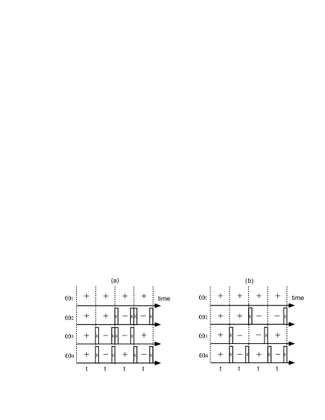
FIG. 1.: (a) Pulse sequence corresponding to Eq.(16). From $S_{4}$, each “$-$” sign in the $i$-th row and $a$-th column translates to two $X$ pulses at $\omega_{i}$ before and after the $a$-th time interval. (b) Pulse sequence obtained from simplifying (a). This corresponds to Eq.(17), and can be constructed directly from $S_{4}$ by translating each change of sign in the $i$-th row to an $X$ pulse at $\omega_{i}$. A “$-$” sign at the end of the row also gives rise to an $X$ pulse at end of the last time interval.

The above scheme can be generalized to decouple $n$ spins with $m$ time intervals as follows:

Construct the $n\times m$ sign matrix $S_{n}$, with entries $+$ or $-$, such that any two rows disagree in exacly half of the entries. For each $-$ sign in the $i$-th row and the $a$-th column, apply $X^{(i)}$ before and after the $a$-th time interval.

Because of the pulses, the sign of the $\sigma_{z}$ matrix for each spin in each time interval is as given by the sign matrix. The $\sigma_{z}$ matrices of any two spins therefore have opposite signs for half of the time, so that their coupling is negated for exactly half of the time, and the evolution is always cancelled.

For $n$ spins, $n\times m$ sign matrices which correspond to decoupling schemes do not necessarily exist for arbitrary $m$, but they always exist for large and special values of $m$. A possible structure is:

$$S_{n}=\left[\begin{array}[]{cccccccccccc}{+}&{\cdots}&{+}&{+}&{\cdots}&{+}&{+}&{\cdots}&{+}&{+}&{\cdots}&{+}\\ {+}&{\cdots}&{+}&{+}&{\cdots}&{+}&{-}&{\cdots}&{-}&{-}&{\cdots}&{+}\\ {}\hfil&{\cdots}&{}\hfil&{}\hfil&{\cdots}&{}\hfil&{}\hfil&{\cdots}&{}\hfil&{}\hfil&{\cdots}&{}\hfil\\ {+}&{\cdots}&{+}&{-}&{\cdots}&{-}&{+}&{\cdots}&{+}&{-}&{\cdots}&{-}\\ {}\hfil&{\cdots}&{}\hfil&{}\hfil&{\cdots}&{}\hfil&{}\hfil&{\cdots}&{}\hfil&{}\hfil&{\cdots}&{}\hfil\\ {+}&{\cdots}&{-}&{+}&{\cdots}&{-}&{+}&{\cdots}&{-}&{+}&{\cdots}&{-}\end{array}\right]\,,$$ (24)

in which intervals are bifurcated when rows (spins) are added. Such bifurcation takes place whenever it is impossible to add an extra row that is orthogonal to all the existing ones (“depletion”). If such depletion occurs frequently, the sign matrix will have exponential number of columns, and decoupling will take exponential number of steps as $n$ increases. The challenge is to find correct sign matrices with subexponential number of columns. This difficult problem turns out to have solutions given by the Hadamard matrices, which will be decribed next.

B Hadamard matrices

Hadamard matrices have applications in many areas such as the construction of designs, error correcting codes and Hadamard transformations [14, 15, 16, 17].

A Hadamard matrix of order $n$, denoted by $H(n)$, is an $n\times n$ matrix with entries $\pm 1$, such that

$$H(n)H(n)^{T}=nI\,.$$ (25)

The rows are pairwise orthogonal, therefore any two rows agree in exactly half of the entries. Likewise columns are pariwise orthogonal. We abbreviate “$\pm 1$” as “$\pm$”. $S_{2}$ and $S_{4}$ in Eqs.(13) and (14) are simple examples of $H(2)$ and $H(4)$. An example of $H(12)$ is given by

$$H(12)=\left[\begin{array}[]{cccccccccccc}{+}&{+}&{+}&{+}&{+}&{+}&{-}&{+}&{+}&{+}&{+}&{+}\\ {+}&{+}&{+}&{-}&{-}&{+}&{+}&{-}&{+}&{-}&{-}&{+}\\ {+}&{+}&{+}&{+}&{-}&{-}&{+}&{+}&{-}&{+}&{-}&{-}\\ {+}&{-}&{+}&{+}&{+}&{-}&{+}&{-}&{+}&{-}&{+}&{-}\\ {+}&{-}&{-}&{+}&{+}&{+}&{+}&{-}&{-}&{+}&{-}&{+}\\ {+}&{+}&{-}&{-}&{+}&{+}&{+}&{+}&{-}&{-}&{+}&{-}\\ {-}&{+}&{+}&{+}&{+}&{+}&{-}&{-}&{-}&{-}&{-}&{-}\\ {+}&{-}&{+}&{-}&{-}&{+}&{-}&{-}&{-}&{+}&{+}&{-}\\ {+}&{+}&{-}&{+}&{-}&{-}&{-}&{-}&{-}&{-}&{+}&{+}\\ {+}&{-}&{+}&{-}&{+}&{-}&{-}&{+}&{-}&{-}&{-}&{+}\\ {+}&{-}&{-}&{+}&{-}&{+}&{-}&{+}&{+}&{-}&{-}&{-}\\ {+}&{+}&{-}&{-}&{+}&{-}&{-}&{-}&{+}&{+}&{-}&{-}\end{array}\right]\,.$$ (38)

The following is a list of useful facts about Hadamard matrices (details and proofs omitted):

1. Equivalence  Permutations or negations of rows or columns of Hadamard matrices leave the orthogonality condition invariant. Two Hadamard matrices are equivalent if one can be transformed to the other by a series of such operations. Each Hadamard matrix is equivalent to a normalized one, which has only $+$’s in the first row and column. For instance, $H(12)$ shown previously can be normalized by negating the 7-${\rm th}$ row and column.

2. Necessary conditions  $H(n)$ exists only for $n=1$, $n=2$ or $n\equiv 0\bmod 4$. This is obvious if the matrix is normalized, and the columns are permuted so that the first three rows become:

   $$\left[\begin{array}[]{cccccccccccc}{+}&{\cdots}&{+}&{+}&{\cdots}&{+}&{+}&{\cdots}&{+}&{+}&{\cdots}&{+}\\ {+}&{\cdots}&{+}&{+}&{\cdots}&{+}&{-}&{\cdots}&{-}&{-}&{\cdots}&{-}\\ {+}&{\cdots}&{+}&{-}&{\cdots}&{-}&{+}&{\cdots}&{+}&{-}&{\cdots}&{-}\\ {\cdot}&{\cdot}&{\cdot}&{\cdot}&{\cdot}&{\cdot}&{\cdot}&{\cdot}&{\cdot}&{\cdot}&{\cdot}&{\cdot}\end{array}\right]\,.$$ (43)

3. Hadamard’s conjecture [18]  $H(n)$ exists for every $n\equiv 0\bmod 4$. This famous conjecture is verified for all $n<428$.

4. Sylvester’s construction [19]  If $H(n)$ and $H(m)$ exist, then $H(nm)$ can be constructed as $H(n)\otimes H(m)$. In particular, $H(2^{r})$ can be constructed as $H(2)^{\otimes r}$, which is proportional to the matrix representation of the Hadamard transformation for $r$ qubits.

5. Paley’s construction [20]  Let $q$ be an odd prime power. If $q\equiv 3\bmod 4$, then $H(q+1)$ exists; if $q\equiv 1\bmod 4$, then $H(2(q+1))$ exists.

6. Numerical facts [14]   For an arbitrary integer $n$, let $\underline{n}$ and $\overline{n}$ be the largest and smallest integers that satisfy $\underline{n}<n\leq\overline{n}$ with known $H(\overline{n})$ and $H(\underline{n})$. We define the “gap”, $\delta_{n}$, to be $\overline{n}-\underline{n}$ (see Fig. 2). For $n\leq 1000$, $H(n)$ is known for every possible order except for 6 cases, and the maximum gap is 8. For $n\leq 10000$, $H(n)$ is unknown for 192 possible orders and the maximum gap is 32.

   

   FIG. 2.: The gap $\delta_{n}$ between two existing orders of Hadamard matrices.

The importance of the full connection to Hadamard matrices will become clear after we construct the scheme for an arbitrary number of spins in the next section.

C General Construction of Scheme

In this section, a decoupling scheme for an arbitrary number of spins is constructed. Variations of the scheme to remove Zeeman evolution and to implement selective recoupling are also constructed. The requirements of the scheme are discussed.

Recall that $\overline{n}$ is the minimum integer no smaller than $n$ with known $H(\overline{n})$, and $m$ is the number of columns in a sign matrix. For any variations of the scheme for $n$ spins, $m_{n}$ is defined to be the minimum number of columns in any valid sign matrix and it represents the number of time intervals needed for the intended operation.

To construct a decoupling scheme for $n$ spins when $H(n)$ does not necessarily exist, any $H(\overline{n})$ with $\overline{n}-n$ rows omitted can be used as the sign matrix since subsets of rows of $H(\overline{n})$ are still pairwise orthogonal. In other words, any $n\times\overline{n}$ submatrix of $H(\overline{n})$ is a valid sign matrix for decoupling $n$ spins, and $m_{n}=\overline{n}$.

To remove both ${\cal H}_{\rm Z}$ and ${\cal H}_{\rm c}$, we use the fact that the Zeeman term for the $i$-th spin is linear in $\sigma_{z}^{(i)}$, and negating $\sigma_{z}^{(i)}$ for half of the time results in no net Zeeman evolution for the $i$-th spin. Therefore, Zeeman evolution for all spins can be removed if the sign matrix has identically zero row sum. Such a sign matrix can be constructed by starting with a normalized $H(\overline{n})$ and excluding the first row of $H(\overline{n})$ in the sign matrix. Since a normalized $H(\overline{n})$ has only $+$’s in the first row, all other rows have zero row sums by orthogonality. Such construction is possible unless $n=\overline{n}$, in which case construction should start with $H(\overline{n+1})$. Therefore, $m_{n}=\overline{n}$ if $n<\overline{n}$ and $m_{n}=\overline{n+1}$ otherwise.

To implement selective recoupling between the $i$-th and the $j$-th spins, the sign matrix should have equal $i$-th and $j$-th rows but any other two rows should be orthogonal. The coupling term $g_{ij}^{\rm c}\sigma_{z}^{(i)}\otimes\sigma_{\rm z}^{(j)}$ never changes sign and that coupling is implemented, while all other couplings are removed. The sign matrix can be obtained from a normalized $H(\overline{n})$ by replacing the $1$-st row with the $j$-th row, and replacing the $j$-th row with the $i$-th row. This scheme also removes ${\cal H}_{\rm Z}$ and $m_{n}=\overline{n}$. To implement $Z\!\!Z_{ij}$, the duration of each interval $t$ is chosen to satisfy $g_{ij}^{\rm c}\overline{n}t=\pi/4$. Note that the total time used to implement $Z\!\!Z_{ij}$ is the shortest possible, since the coupling is always “on”.

The scheme requires $m_{n}$ time intervals. Consequently, it requires at most $nm_{n}$ pulses, since $XX=I$ and the $X$ pulses are only used in pairs. The remaining question is: how does $m_{n}$ depend on $n$? For simplicity, we consider $\overline{n}$ in place of $m_{n}$. If Hadamard matrices exist and can be constructed for all orders, $\overline{n}=n$. However, some Hadamard matrices are missing, either because no construction methods are known or they simply cannot exist. Due to missing Hadamard matrices, $\overline{n}=cn$ where $c\geq 1$. We argue in the following that the scheme is still very efficient. First of all, we prove $c<2$. For each $n$, there exists $r$ such that $2^{r-1}\!\leq n<2^{r}$. Since $H(2^{r})$ exists by Sylvester’s construction, $cn=\overline{n}\leq 2^{r}\!\!<2n$. We now show that $c$ is close to the ideal value 1 in most cases, due to the existence of Hadamard matrices of orders other than powers of 2. This is why the full connection to Hadamard matrices is important. In Fig. 3, $c$ as a function of $n$ is plotted for $n\leq 10000$. Within this technologically relevant range of $n$, $c$ deviates significantly from 1 only for a few exceptional values of $n$ when $n$ is small. One arrives at the same conclusion by considering the gap $\delta_{n}=\overline{n}-\underline{n}>\overline{n}-n$, which bounds the extra number of intervals needed in the scheme caused by missing Hadamard matrices. For $n\leq 10000$, $\delta_{n}/n\ll 1$ except for the few exceptional values of $n$ as a numerical fact. For completeness, we present arguments for $c\approx 1$ for arbitrarily large $n$ in Appendix A. This is based on Paley’s construction and the prime number theorem. Finally, if Hadamard’s conjecture is proven, $\delta_{n}\leq 3$ $\forall n$.

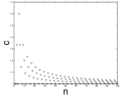
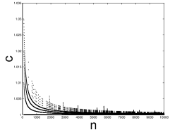
FIG. 3.: Plots of $c$ vs $n$, where $cn=\overline{n}=m_{n}$ is the minimun number of time intervals required to perform decoupling or selective recoupling for an $n$-spin system. $c$ for $n\leq 100$ and $101\geq n\leq 10000$ are plotted separately.

IV Conclusion

We reduce the problem of decoupling and selective recoupling in heteronuclear spin systems to finding sign matrices which is further reduced to finding Hadamard matrices. While the most difficult task of constructing Hadamard matrices is not discussed in this paper, solutions already exist in the literature. Even more important is that the connection to Hadamard matrices results in very efficient schemes.

Some properties of the scheme are as follows. First of all, the scheme is optimal in the following sense. The rows of Hadamard matrices and their negations form the codewords of first order Reed-Muller codes, which are perfect codes [16, 17]. It follows that, for each Hadamard matrix, it is impossible to add an extra row which is orthogonal to all the existing ones. Therefore, for a given $n$, $m_{n}=\overline{n}$ is in fact the minimum number of time intervals necessary for decoupling or recoupling, if one restricts to the class of pulse sequences considered. Second, the scheme applies for arbitrary duration of the time intervals. This is a consequence of the commutivity of all the terms in the hamiltonian, which in turn comes from the large separations of the Zeeman frequencies compared to the coupling constants. Spin systems can be chosen to satisfy this condition. Finally, disjoint pairs of spins can couple in parallel.

We outline possible simplifications of the scheme for systems with restricted range of coupling. For example, a linear spin system with $n$ spins but only $k$-nearest neighbor coupling can be decoupled by a scheme for $k$ spins only. The $i$-th row of the $n\times\overline{k}$ sign matrix can be chosen to be the $r$-th row of $H(\overline{k})$, where $i\equiv r\bmod k$. Selective recoupling can be implemented using a decoupling scheme for $k+1$ spins. The sign matrix is constructed as in decoupling using $H(\overline{k+1})$ but the rows for the spins to be coupled are chosen to be the $k+1$-th row different from all existing rows [21]. This method involving periodic boundary conditions generalizes to other spatial structures. The size of the scheme depends on $k$ and the exact spatial structure but not on $n$.

The scheme has several limitations. First of all, it only applies to systems in which spins can be individually addressed by short pulses and coupling has the simplified form given by Eq.(4). These conditions are essential to the simplicity of the scheme. They can all be satisfied if the Zeeman frequencies have large separations. Second, generalizations to include couplings of higher order than bilinear remain to be developed. Furthermore, in practice, RF pulses are inexact and have finite durations, leading to imperfect transformations and residual errors.

The present discussion is only one example of a more general issue, that the naturally occuring hamiltonian in a system does not directly give rise to convenient quantum logic gates or other computations such as simulation of quantum systems [22]. Efficient conversion of the given system hamiltonian to a useful form is necessary and is an important challenge for future research.

V Acknowledgments

This work was supported by DARPA under contract DAAG55-97-1-0341 and Nippon Telegraph and Telephone Corporation (NTT). D.L. acknowledges support of an IBM Co-operative Fellowship. We thank Hoi-Fung Chau, Kai-Man Tsang, Hoi-Kwong Lo, Alex Pines, Xinlan Zhou and Lieven Vandersypen for helpful comments.

A Upper bounds for $\overline{n}$

An argument for $c\approx 1$ for large $n$ is presented using Paley’s construction (mentioned in Section III B), known results on primes in intervals and the prime number theorem for arithmetic progressions.

Let $\pi(x)$ be the number of primes which satisfy $2\leq p\leq x$. For $x<67$, $x/(\log x-1/2)<\pi(x)<x/(\log x-3/2)$ [23]. It follows that there exists a prime between $n$ and $n(1+\epsilon)$ for $\epsilon>2/\log n$. Applying Paley’s construction, $H(p+1)$ or $H(2(p+1))$ exists depending on whether $p\equiv 3\bmod 4$ or $p\equiv 1\bmod 4$. Therefore, $\overline{n}\leq n(1+\epsilon)+1$ or $\overline{n}\leq 2(n(1+\epsilon)+1)$ respectively.

The worse of the upper bounds $\overline{n}\leq 2(n(1+\epsilon)+1)$ resulting from $p\equiv 1\bmod 4$ can be improved. Note that there are at least $r$ primes between $n$ and $n(1+\epsilon)^{r}$. If the primes that equal $3\bmod 4$ and $1\bmod 4$ are randomly and uniformly distributed, the probability to find a prime which equals $3\bmod 4$ between $n$ and $n(1+\epsilon)^{r}$ is larger than $1-2^{-r}$. This assumption is true due to the prime number theorem for arithmetic progressions [24]. Let $\pi(x,a,q)$ denotes the number of primes in the arithmetic progression $\{a,a+q,a+2q,\ldots\}$ which satisfy $2\leq p\leq x$. It is known that $\pi(x,3,4)\approx\pi(x,1,4)$. Therefore, with probability larger than $1-2^{-r}$, $\overline{n}\leq n(1+\epsilon)^{r}+1$, implying $c\leq(1+\epsilon)^{r}+1/n\approx 1$ for large $n$.

REFERENCES

- [1] N. Gershenfeld and I. Chuang, Science 275, 350 (1997).
- [2] D. Cory, A. Fahmy and T. Havel, Proc. Natl Acad. Sci. USA 94, 1634-1639 (1997).
- [3] D. Cory, M. Price and T. Havel, Physica D, in print (1997), also LANL E-print quant-ph/9709001, (1997).
- [4] I. Chuang, N. Gershenfeld, M. Kubinec, and D. Leung, Proc. R. Soc. Lond. A (1998) 454, 447-467.
- [5] R. Josza, Proceedings of First NASA International Conference on Quantum Computation and Quantum Communication (Palm Springs, February 1998), also LANL E-print quant-ph/9805086, (1998).
- [6] R. R. Ernst, G. Bodenhausen, and A. Wokaun, Principles of Nuclear Magnetic Resonance in One and Two Dimensions (Oxford University Press, Oxford, 1994).
- [7] C. Slichter, Principles of Magnetic Resonance (Springer, Berlin, 1990).
- [8] P. Mansfield, Pulsed NMR in Solids Progress in Nuclear Magnetic Resonance Spectroscopy Vol. 8 (Pergamon Press, Oxford, 1971).
- [9] N. Linden, H. Barjat, R. Carbajo and R. Freeman, LANL E-print quant-ph/9811043, (1998). Homonuclear systems were considered, in contrast to the present discussion.
- [10] D. DiVincenzo, Phys. Rev. A. 51, 1015, (1995).
- [11] A. Barenco, Proc. R. Soc. Lond. A (1995) 449, 679-83.
- [12] D. Deutsch, A. Barenco and A. Ekert, Proc. R. Soc. Lond. A (1995) 449, 669-77.
- [13] A. Abragam, The Principles of Nuclear Magnetism (Oxford University Press, Oxford, 1961).
- [14] C. Colbourn and J. Dinitz (Eds) The CRC Handbook of Combinatorial Designs (CRC Press, Boca Raton, 1996).
- [15] http://www.research.att.com/njas/hadamard/index.ht-ml
- [16] J. van Lint and R. Wilson, A Course in Combinatorics (Cambridge University Press, Cambridge, 1992).
- [17] F. MacWilliams and N. Sloane, The theory of Error-Correcting Codes (North Holland, Amsterdam, 1977).
- [18] J. Hadamard, Bull. Sciences Math., (2) 17 (1893), 240-246.
- [19] J. Sylvester, Phil. Mag. 34 (1867), 461-475.
- [20] R.E.A.C Paley, J. Math. Phys. 12 (1933), 311-320.
- [21] With a periodic sign matrix, setting the -th row to be the -th row also recoupling the -th and the -th spins when . Similar problem occurs when . Therefore a row different from all existing ones is used. This is not necessary in linear systems using a more complicated scheme, but it is necessary for other structures such as a planar system.
- [22] B. Terhal and D. DiVincenzo, LANL E-print quant-ph/9810063, (1998).
- [23] J. Rosser and L. Schoenfeld, Illinous J. Math. 6 (1962), 64-94.
- [24] H. Davenport, Multiplicative Number Theory, (Springer-Verlag, New York, 1967).