Generation of entanglement in a system of two dipole-interacting atoms by means of laser pulses

Abstract

Effectiveness of using laser field to produce entanglement between two dipole-interacting identical two-level atoms is considered in detail. The entanglement is achieved by driving the system with a carefully designed laser pulse transferring the system’s population to one of the maximally entangled Dicke states in a way analogous to population inversion by a resonant $\pi$-pulse in a two-level atom. It is shown that for the optimally chosen pulse frequency, power and duration, the fidelity of generating a maximally entangled state approaches unity as the distance between the atoms goes to zero.

With recent experimental advances in the methods for coherent manipulation of quantum system on the level of individual particles, many of previously purely speculative problems become surprisingly up-to-date. In particular, much activity of physicists from different research fields is currently devoted to clarification of the entanglement concept [1], ways for its quantification, purification, and creation. Casual creation of entangled states of atoms by coherent manipulation with light currently poses one of the biggest challenges in the field of quantum optics [2]. Conversely, the resonant dipole-dipole interaction (RDDI) and cooperative relaxation effects associated with it are rather traditional topics of research. Recently the RDDI has been investigated as a source of interference phenomena in emission spectra [3, 4, 5], super- and sub-radiance [6, 7], photon bunching [8], collisions in the laser cooling processes [9, 10], and as a mechanism for realizing quantum logical gates [11, 12]). In this paper we address the question: how effectively can the RDDI along with coherent laser pulses be used for creation of multi-atomic entangled states.

In our model two identical two-level atoms are located at a fixed distance $R$ and can be driven by laser beam that is either parallel or perpendicular (according to geometries identified, respectfully, as antisymmetric and symmetric, Fig. 1) to the radius vector $\vec{R}$ connecting the atoms. Within the interaction picture and rotating wave approximation, the evolution is described by the following master equation [5]:

$$\frac{\partial\hat{\rho}}{\partial t}=-\frac{i}{h}\left[\hat{\cal H}_{\rm eff},\rho\right]+\sum_{i,j=1,2}\frac{\gamma_{ij}}{2}(2\hat{\sigma}^{-}_{i}\hat{\rho}\hat{\sigma}^{+}_{j}-\hat{\rho}\hat{\sigma}^{-}_{i}\hat{\sigma}^{+}_{j}-\hat{\sigma}^{-}_{i}\hat{\sigma}^{+}_{j}\hat{\rho}),$$ (1)

where

$$\hat{\cal H}_{\rm eff}=\frac{\hbar}{2}\left[-\delta\left(\hat{\sigma}^{z}_{1}+\hat{\sigma}^{z}_{2}\right)+\Omega_{1}\hat{\sigma}^{+}_{1}+\Omega_{2}\hat{\sigma}^{+}_{2}+\chi\hat{\sigma}^{+}_{1}\hat{\sigma}^{-}_{2}+\mbox{h.\,c.}\right].$$ (2)

is the effective Hamiltonian describing the atoms’ self-evolution and interaction with the laser field. Here $\delta=\omega_{L}-\omega_{a}$ is the laser detuning from the atomic transition frequency, $\Omega_{1,2}$ are the complex laser driving Rabi frequencies for each atom, $\hat{\sigma}^{x}_{i},\,\hat{\sigma}^{y}_{i},\,\hat{\sigma}^{z}_{i},\,\hat{\sigma}^{\pm}_{i}=\hat{\sigma}^{x}_{i}\pm i\hat{\sigma}^{y}_{i},\,i=1,2,$ are (using the well-known analogy between two-level atoms and spins) the spin-$\frac{1}{2}$ Cartesian component and transition operators of the $i$-th atom, and we define $g$, $f$ and $\gamma$ so that $\gamma_{11}=\gamma_{22}=\gamma,\,\gamma_{12}=\gamma_{21}=g\gamma,\,\chi=f\gamma$. The distance dependent parameters $g$ and $f$, describing, respectfully, the photon exchange rate and coupling due to the RDDI, are defined differently for different types of the atomic transition in question. Defining $p=0,\,q=2$ for $\Delta m=0$ and $p=1,\,q=-1$ for $\Delta m=\pm 1$ transitions (with the quantization axis coinciding with $\vec{R}$) and assuming that dipole matrix elements of the atoms are collinear to each other and perpendicular to $\vec{R}$, we have the following expressions for $g(\varphi)$ and $f(\varphi)$ [13]:

$$g(\varphi)=\frac{3}{2}\left(p\frac{\sin\varphi}{\varphi}+q\frac{\sin\varphi}{\varphi^{3}}-p\frac{\cos\varphi}{\varphi^{2}}\right),\quad f(\varphi)=\frac{3}{2}\left(p\frac{\cos\varphi}{\varphi}+q\frac{\cos\varphi}{\varphi^{3}}+q\frac{\sin\varphi}{\varphi^{2}}\right),$$ (3)

where $\varphi=kR$ is the “dimensionless distance” between the atoms and $k=\omega_{a}/c$. Throughout the rest of the article we will consider $\Delta m=\pm 1$ case for determinacy as for the $\Delta m=0$ case the results are qualitatively same.

It can easily be shown that the Dicke states, $\mathop{\left|\psi_{e}\right\rangle}\nolimits=\mathop{\left|e\right\rangle}\nolimits_{1}\mathop{\left|e\right\rangle}\nolimits_{2},\,\mathop{\left|\psi_{g}\right\rangle}\nolimits=\mathop{\left|g\right\rangle}\nolimits_{1}\mathop{\left|g\right\rangle}\nolimits_{2},\,\mathop{\left|\psi_{s}\right\rangle}\nolimits=\frac{1}{\sqrt{2}}(\mathop{\left|g\right\rangle}\nolimits_{1}\mathop{\left|e\right\rangle}\nolimits_{2}+\mathop{\left|e\right\rangle}\nolimits_{1}\mathop{\left|g\right\rangle}\nolimits_{2})$, and $\mathop{\left|\psi_{a}\right\rangle}\nolimits=\frac{1}{\sqrt{2}}(\mathop{\left|g\right\rangle}\nolimits_{1}\mathop{\left|e\right\rangle}\nolimits_{2}-\mathop{\left|e\right\rangle}\nolimits_{1}\mathop{\left|g\right\rangle}\nolimits_{2})$ (where $\mathop{\left|e\right\rangle}\nolimits_{i}$ and $\mathop{\left|g\right\rangle}\nolimits_{i}$ are the upper and lower levels of the $i$th atom) are the eigenvectors of $\hat{\cal H}_{\rm eff}$ (when excluding the laser driving), while the rest of the atomic dynamics can be described as radiative decay to/from the antisymmetric $\mathop{\left|\psi_{a}\right\rangle}\nolimits$ state with the rate $\gamma_{-}=(1-g)\gamma$ and to/from the symmetric $\mathop{\left|\psi_{s}\right\rangle}\nolimits$ one with the rate $\gamma_{+}=(1+g)\gamma$.

Analytical stationary solutions of (1) can be found for the case of symmetric excitation $\Omega_{1}=\Omega_{2}=\Omega$ (without loss of generality we can assume that $\Omega$ here is real and positive) with the stationary populations of the Dicke states given by

$$\begin{array}[]{c}\displaystyle N_{e}=N_{a}=\frac{\Omega^{4}}{\left(\gamma^{2}+4\delta^{2}+2\Omega^{2}\right)^{2}+\gamma(\gamma^{2}+4\delta^{2})(f^{2}\gamma+g^{2}\gamma+2g\gamma-4f\delta)},\\ \displaystyle N_{s}=\frac{2\Omega^{2}(2\gamma^{2}+8\delta^{2}+\Omega^{2})}{\left(\gamma^{2}+4\delta^{2}+2\Omega^{2}\right)^{2}+\gamma(\gamma^{2}+4\delta^{2})(f^{2}\gamma+g^{2}\gamma+2g\gamma-4f\delta)},\\ N_{g}=1-N_{e}-N_{a}-N_{s}.\end{array}$$ (4)

Graph $N_{s}(\Omega,\delta)$, corresponding to $\varphi=0.5$, is shown in Fig. 2a. The antisymmetric case, when the laser beam is parallel to $\vec{R}$, allows no such simple analytical solution since in this case the relation between the Rabi frequencies for two atoms is more complex $\Omega_{1}=e^{i\varphi}\Omega_{2}=\Omega$ (although $\Omega$ here is again real and positive). However, the numerical solution is easily obtained and the corresponding dependence $N_{a}(\Omega,\delta)$ is shown in Fig. 2b.

If we aim to transfer the maximum amount of population into one of the maximally entangled states $\mathop{\left|\Psi_{a}\right\rangle}\nolimits$ or $\mathop{\left|\Psi_{s}\right\rangle}\nolimits$ by a short coherent pulse, a good criterion for finding optimal values of the laser field parameters, $\Omega$ and $\delta$, is whether the population of the corresponding level is close to 0.5 in the stationary solution. From the analysis of (4) and the graphs in Fig. 2 we deduce that the optimal parameters can be well approximated by $\delta_{opt}=\pm\chi(\varphi)/2$ and $\Omega_{opt}=\sqrt{|\chi(\varphi)|\gamma_{\pm}}$ with the upper/lower sign for the symmetric/antisymmetric geometries, respectfully. We then have $|\delta_{opt}|=|\chi|/2\gg\Omega_{opt}\gg\gamma_{\pm}$ for sufficiently small distances, so that the transition of interest is saturated while at the same time the Rabi frequency is moderate enough to avoid broadband excitation of the Dicke level we are not interested in.

Given the optimal parameters obtained in the previous section we proceed to find the fidelity of creation of the maximally entangled states, that is the maximum amount of population one can transfer using pulses of radiation. Considering the dynamics of the populations under optimal parameters laser driving that is turned on at the time instant $t=0$ (when all of the population is in $\mathop{\left|\Psi_{g}\right\rangle}\nolimits$ state), we define the optimal pulse duration as the time when the population of the state we are interested in, reaches its first maximum. For the so chosen parameters we plot in Fig. 3a the populations achieved by applying the optimal pulse, as a function of interatomic distance $\varphi$. The populations approach unity for both geometries as $\varphi$ goes to zero suggesting that almost perfect transfer of population is attainable at small interatomic distances.

It is easy to explain this result. As $R$ goes to zero the energy splitting between the symmetric and antisymmetric state, equal to $2\chi=2f\gamma$, grows to infinity (of course, within the evident limitations of negligibility of exchange effects [5]). The “parasitic” excitation of the levels we are not interested in is then avoided by shifting the laser frequency so that we are in resonance only with one of the excited Dicke states. And if we have in possession arbitrarily strong and arbitrarily tunable laser, as $\varphi$ goes to zero we can produce shorter and shorter pulses thereby decreasing the decay probability during the pulse.

In addition, in the case of the symmetric excitation laser driving matrix element for the transitions involving the antisymmetric state vanishes. This means that its population can only come from decay of the upper $\mathop{\left|\Psi_{e}\right\rangle}\nolimits$ level. In fact, in the stationary solution (4) the two states even have the same populations, which are negligible for large detunings. In the antisymmetric excitation case, however, the situation works against us. As the interatomic distance goes to zero the Rabi frequencies of the two atoms become closer in phase, diminishing along the way the matrix elements of transitions involving antisymmetric state to zero. But even with such a small value of excitation efficiency, we can still manage to transfer the population to the antisymmetric state because the symmetric excitation remains far off resonance, and get as a reward the increased lifetime $\tau=1/\left((1-g(R))\gamma\right)\gg 1/\gamma$ of our maximally entangled state (using this “durability” of the antisymmetric $\mathop{\left|\Psi_{a}\right\rangle}\nolimits$ state, we can also create some entanglement passively as described in [14], but it is difficult to obtain a high fidelity that way).

Now, instead of calculating different entanglement measures [15] (and then figuring out which of them better suits our purposes), we will consider how much our created states violate a simple Bell inequality. It can be easily shown [1] that for any classical local variable distribution the probabilities of finding the atoms’ “spins” aligned along $\vec{n}_{z}$ direction after coherent rotations fulfill the following Bell inequality:

$$P_{\rm diff}(0,2\pi/3)+P_{\rm diff}(2\pi/3,-2\pi/3)+P_{\rm diff}(0,-2\pi/3)\geq 1,$$ (5)

where the $P_{\rm diff}(\varphi_{1},\varphi_{2})$ is the probability of getting different results of the measurements of the two spins, i.e., of finding one spin aligned along the $\vec{n}_{z}$ direction and the second one against it after the first spin is rotated by $\varphi_{1}$ and the second one by $\varphi_{2}$ around $OX$ or $OY$ axis. In quantum mechanics, however, the left hand side of (5) amounts to only 0.75 for the pure maximally entangled $\mathop{\left|\Psi_{a}\right\rangle}\nolimits$ state. To apply the same Bell inequality (5) to the case of the symmetric excitation geometry we first perform a $180^{\circ}$ rotation along $\vec{n}_{z}$-axis with one of the atoms (thus turning $\mathop{\left|\Psi_{s}\right\rangle}\nolimits$ state into $\mathop{\left|\Psi_{a}\right\rangle}\nolimits$ one) and then perform the measurement as described above. In Fig. 3b the l.h.s. of (5) is plotted against the dimensionless distance $\varphi$ showing that for $\varphi$ less than $\approx 0.5$ we have the violation of the inequality and as $\varphi\rightarrow 0$ we recover the pure states limit of 0.75.

In summary, while being admittedly unrealistic, our model offers a few insights into how efficiently the RDDI can be used to entangle atoms or implement quantum logic gates [12, 16]. We have shown that considerable fidelities (up to 0.8) of creation of one of the maximally entangled Dicke states and Bell inequality violations can be realized if the atoms are placed within distances of the order of a tenth of a wavelength of the working transition. Such distances can be achieved, for example, in the ground vibrational states of two atoms in optical lattices [10, 12, 17].

However, all of the practical applications (say, quantum teleportation [18]) require stable entanglement. Even the Bell inequalities violation considered above can be verified only if the produced entanglement lives sufficiently long so that the atoms can be spatially separated for individual addressing and photodetection (imperfectness of the detectors constitutes another problem that has not yet been addressed). Of course, this cannot be achieved in our model, since the dipole interaction and the decay have the same physical nature and we cannot avoid the latter while making use of the former.

Relatively stable coherences (with lifetimes of the order of seconds) can be generated if we use the Zeeman sublevels of the atoms as the working levels (qubits). The RDDI is negligible for them, but using three-level atoms in $\Lambda$-configuration instead of two-level atoms we can overcome that difficulty. We can use Raman pulses transferring the population between the Zeeman sublevels via a higher lying “transit” Dicke level (STIRAP techniques [19] might be an alternative), so that the transitions between each of the Zeeman sublevels states and the excited “transit” state benefit from substantial RDDI. Then by choosing one-photon detunings to be in resonance with only one of the higher level Dicke states we can generate the Zeeman sublevels entanglement.

In this paper we present the first tentative quantitative model of the process of entanglement of atoms with the help of the RDDI. Much remains to be done before we can compare the results of the theory with possible practical implementations, but the conclusions presented here are promising and therefore encourage further theoretical developments.

This work was partially supported by Volkswagen Stiftung (grant No. 1/72944) and the Russian Ministry of Science and Technical Policy.

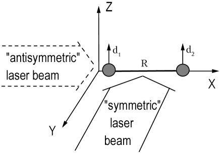
FIG. 1.: Geometry of the model with shown directions of laser beams for the symmetric and antisymmetric excitation.

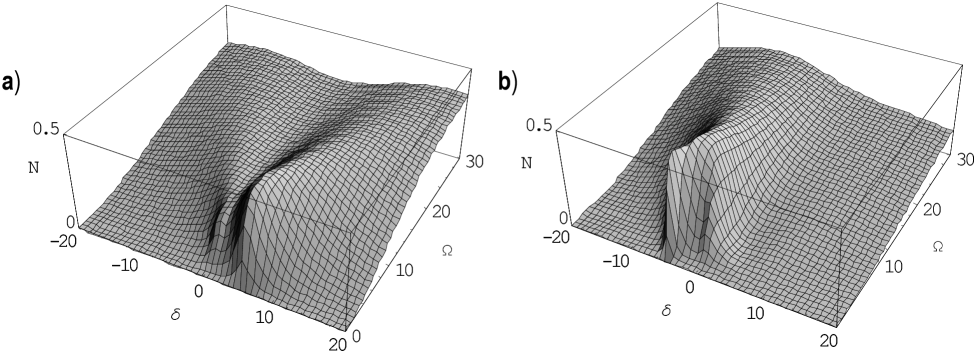
FIG. 2.: The stationary populations of the symmetric (a) and antisymmetric (b) Dicke states versus the laser detuning $\delta$ and the laser driving Rabi frequency $\Omega$ for $\varphi=0.5$.

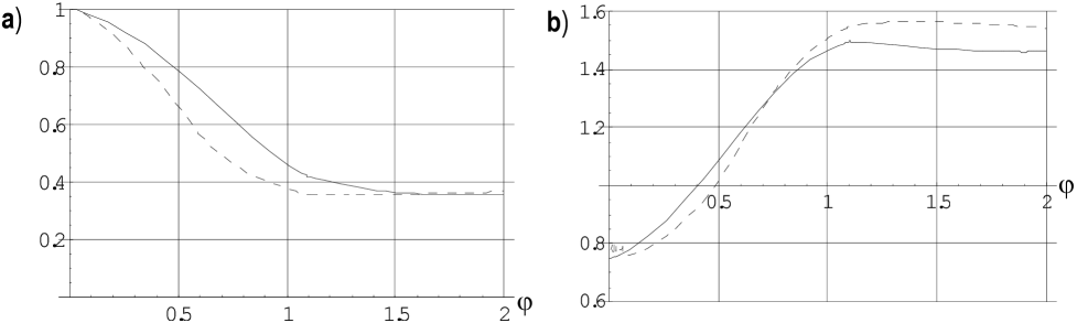
FIG. 3.: a) The fidelity of creation of the maximally entangled states (by applying the optimal pulse as described in text) versus interatomic distance $\varphi$. b) The l.h.s. of the Bell inequality (5) versus $\varphi$. The pure states limit is 0.75, uncorrelated states lead to 1.5, the classical boundary is 1.0. Solid and dashed lines correspond to the antisymmetric and symmetric cases, respectfully.

REFERENCES

-
[1]
See, e. g., John Preskill, Lecture notes on Physics 229: Quantum
information and computation, located at Caltech web site
http://www.theory.caltech.edu/people/preskill/ph229/index.html. - [2] C. Cabrillo, J.I. Cirac, P. Garcia-Fernandez, and P. Zoller, Phys. Rev. A 59 (1999) 1025; M. B. Plenio, S. F. Huelga, A. Beige, P. L. Knight, Phys. Rev. A 59 (1999) 2468; Q. A. Turchette, C. S. Wood, B. E. King, C. J. Myatt, D. Leibfried, W. M. Itano, C. Monroe, D. J. Wineland, Phys. Rev. Lett. 81 (1998) 3631; D. Jaksch, H.-J. Briegel, J.I. Cirac, C.W.Gardiner, and P. Zoller, Phys. Rev. Lett. 82 (1999) 1975.
- [3] G.S. Agarwal and L.M. Narducci, E. Apostolidis, Opt. Comm. 36 (1981) 285.
- [4] Georg Lenz and Pierre Meystre, Phys. Rev.A 48 (1993) 3365.
- [5] Gershon Kurizki and Abraham Ben-Reuven, Phys. Rev. A 36 (1987) 90.
- [6] R.G. Brewer, Phys. Rev. A 52 (1995) 2965.
- [7] A.V. Andreev, V.I. Emel’yanov, Yu. A. Il’inskii, Cooperative effects in optics: superradiance and phase transitions, Philadelphia, PA: Institute of Physics Publishing, 1993.
- [8] Almut Beige and Gerhard C. Hegerfeldt, Phys. Rev. A 58 (1998) 4133.
- [9] A.M. Smith and K. Burnett, J. Opt. Soc. Am. B 8 (1991) 1592.
- [10] E.V. Goldstein, P. Pax and P. Meystre, Phys. Rev. A 53 (1996) 2604.
- [11] Adriano Barenco, David Deutsch, Arthur Ekert, Richard Jozsa, Phys. Rev. Lett. 74 (1995) 4083.
- [12] Gavin K. Brennen, Carlton M. Caves, Poul S. Jessen and Ivan H. Deutsch, Phys. Rev. Lett. 82 (1999) 1060.
- [13] P.W. Milloni and P. L. Knight, Phys. Rev. A 10 (1974) 1096.
- [14] B.A. Grishanin, V.N. Zadkov, Laser Physics 8 (1998) 1074.
- [15] Jens Eisert, Martin B. Plenio, quant-ph/9807034.
- [16] D. Deutsch, A. Barenco, A. Ekert, Proc. Roy. Soc. of London A 449 (1995) 669.
- [17] H. Wallis, Phys. Rep. 255 (1995) 203.
- [18] Charles H. Bennett, Gilles Brassard, Claude Crepeau, Richard Jozsa, Asher Peres, and Willam K. Wooters, Phys. Rev. Lett. 70 (1993) 1895.
- [19] K. Bergmann, H. Theuer, and B. W. Shore, Rev. Mod. Phys. 70 (1998) 1003.